Regularised inference for changepoint and dependency analysis in non-stationary processes

(1)

Regularised Inference for Changepoint

and Dependency Analysis in

Non-Stationary Processes

Alexander James Gibberd

A dissertation submitted in partial fulfillment of the requirements for the degree of

Doctor of Philosophy of

University College London

Department of Statistical Science Department of Security and Crime

Science

September 2017

(2)

(3)

3

I, Alexander James Gibberd confirm that the work presented in this thesis is my own. Where information has been derived from other sources, I confirm that this has been indicated in the thesis.

(4)

(5)

5

Abstract

Multivariate correlated time series are found in many modern socio-scientific domains such as neurology, cyber-security, genetics and economics. The focus of this thesis is on efficiently modelling and inferring dependency structure both between data-streams and across points in time. In particular, it is considered that generating processes may vary over time, and are thus non-stationary. For example, patterns of brain activity are expected to change when performing different tasks or thought processes.

Models that can describe such behaviour must be adaptable over time. However, such adaptability creates challenges for model identification. In order to perform learning or estimation one must control how model complexity grows in relation to the volume of data. To this extent, one of the main themes of this work is to investigate both the implementation and effect of assumptions on sparsity; relating to model parsimony at an individual time-point, and smoothness; how quickly a model may change over time.

Throughout this thesis two basic classes of non-stationary model are stud-ied. Firstly, a class of piecewise constant Gaussian Graphical models (GGM) is introduced that can encode graphical dependencies between data-streams. In particular, a group-fused regulariser is examined that allows for the estima-tion of changepoints across graphical models. The second part of the thesis focuses on extending a class of locally-stationary wavelet (LSW) models. Un-like the raw GGM this enables one to encode dependencies not only between data-streams, but also across time. A set of sparsity aware estimators are developed for estimation of the spectral parameters of such models which are then compared to previous works in the domain.

(6)

(7)

7

Note on Writing Style

This thesis predominantly follows a third person narrative, where through-out this thesis I use “we” to relate to the reader and myself. At some places I use the term “I” to relate to my own thoughts and beliefs.

List of Publications

This thesis is based in part on the following papers which are published in peer-reviewed journals/proceedings:

• A. Gibberd and J.D.B Nelson, ‘Group-fused Graphical Lasso for Change-point estimation in Multivariate Time-series’,IMA International Con-ference on Mathematics in Signal Processing, 2014

• A. Gibberd and J.D.B Nelson, ‘High Dimensional Changepoint Detec-tion with a Dynamic Graphical Lasso’,IEEE International Conference on Acoustics, Speech, and Signal Processing, 2014

• A. Gibberd and J.D.B Nelson, ‘Sparsity in the Multivariate Wavelet Framework: A Comparative Study Using Epileptic Electroencephalog-raphy Data’, IET Intelligent Signal Processing, 2015 (Chapter 6)

• A. Gibberd and J.D.B Nelson. ‘Estimating Multi-Resolution Depen-dency Graphs within a Locally Stationary Wavelet Framework’,IEEE Global Conference on Signal & Information Processing, 2015 (Chapter 6)

• A. Gibberd and J.D.B Nelson, ‘Regularised Estimation of 2D-Locally Stationary Wavelet Processes’, IEEE Workshop on Statistical Signal Processing, 2016 (Chapter 6)

• A. Gibberd and J.D.B Nelson, ‘Estimating Dynamic Graphical Models from Multivariate Time-Series Data: Recent Methods and Results’, Lecture Notes on Artificial Intelligence, 2016 (Chapters 2, 3)

• A. Gibberd and J.D.B. Nelson, ‘Regularized Estimation of Piecewise Constant Gaussian Graphical Models: The Group-Fused Graphical Lasso’,Journal of Computational & Graphical Statistics, 2017 (Chap-ter 3)

• A. Gibberd, M. Evangelou and J.D.B. Nelson, ‘The Time-Varying De-pendency Patterns of NetFlow Statistics’,IEEE International Confer-ence on Data Mining, 2016 (Chapter 3)

(8)

(9)

9

(10)

(11)

11

Acknowledgements

First and foremost, I would like to dedicate this thesis to my late supervisor Dr James Nelson: Without James’ unique mix of patience, creativity and passion for knowledge this thesis would never have been completed. I am, and always will be grateful for the time, freedom, and opportunities he afforded me throughout our time working together.

A very special gratitude goes to Defence Science Technology Laboratory (DSTL) for funding this work, and especially to Ralph for being so hospitable and the great discussions. I would also like to thank my second supervisor Ricardo Silva, collaborators; Matt Nunes, Sandipan Roy, Marina Evangelou, Niall Adams, and Marcela Mendoza. Thanks to Alex Immer for helping me navigate the horrors of entrepreneurship. Thanks to Robbie for helping with the proofreading effort.

Equally, while there are many who have helped me with my research, there are many more I am grateful for making my time as a PhD actually enjoyable! I’m eternally thankful to have had the Luncheon crew to provide a constant source of mid-day procastrination, coffee, and beer drinking. To all the guys in the stats office, I’m not sure how much work I actually did at my office (at that rate I should also thank the staff of Costa), but it was always a fun place to be. I’d also like to say thanks for JB and Hojjat for all the travels and chats, especially towards the end.

Last but not least, I am grateful for the continued and unconditional sup-port of my family; June, Al, Ham, and Josie. Also a big shout out to Auntie Sue and Uncle Ray who helped me stave off starvation while writing this doc-ument. Finally, I really want to thank Anastasia for all the care, love and food she has provided throughout the process of writing this document. I’m very much looking forward to spending weekends together again.

(12)

(13)

Chapter 1 Introduction

High-dimensional correlated time-series are ubiquitous in many real world ap-plications, from observations of how blood flows throughout the brain to under-standing traffic flows across computer networks. The continuous development of sensing technologies places new requirements on the tools and methodologies that are used to gain understanding from data. Not only are new datasets ac-quired faster, and in greater resolutions, but they also measure more aspects of the world around us. In many applications, the number of features or variables that one may measure often outnumber the volume of points at which these may be sampled. Such high-dimensional situations pose serious challenges for statistical estimation due to the inherently large number of degrees of freedom associated with traditional models.

To avoid overfitting, in the high-dimensional setting one is required to make assumptions about the dynamics and dependency of variables. Typically, these will be encoded by a statistical model. However, even for very simple statis-tical models like linear regression, the number of model parameters may grow faster than data can be collected. To enable estimation of the model, it is often assumed that the data may be described by a smaller subset of the parame-ters required in the ambient dimension. While such assumptions help stabilise our model statistically; they give rise to challenges in computation associated with how we search the model space for the best set of parameters. These challenges are inextricably linked. For example, certain statistical models and assumptions allow for a simplified computational search, but potentially at the

(20)

expense of statistical performance. The assumptions that we make in order to identify a model often affect the level of insight one may obtain from the underlying data. It is therefore of paramount importance to consider the the-oretical and empirical consequences of assumptions, both in a computational and statistical sense.

1.1 Motivational Applications

To give an idea of how and where methods developed in the thesis may be used, we here discuss two areas of critical importance to society; namely, neuroscience, and cyber-security. Both of these applications are examined to various depths further in the thesis, particularly, Sections 3.4 and 7.4.

1.1.1 Understanding Brain Activity

There are several neuroscientific objectives associated with the analysis of neurological data. For example, one may be interested in localising regions of the brain linked to certain tasks, determining how regions of the brain interact (functional mapping), or making predictions about psychological or disease status. In this thesis, the primary topic of interest is modelling dependency structure between variables; concerning neurological analysis this strongly re-lates to the objective of functional mapping within the brain. Specifically, if one represents the relationships between parts of the brain as a network, then robustly inferring this network structure is of paramount importance. Not only do the methods of this thesis aim to address the challenge of infering network strcutre, but also extend this to the setting where these dependencies can evolve over time.

Several forms of sensing technology may be used to measure brain activity: techniques such asmagnetoencephalography (MEG)andelectroencephalography (EEG) rely on sensing the magnetic and electrical activity within the brain, whereas functional magnetic resonance imaging (fMRI) data uses blood flow in the brain as a proxy for activity.

(21)

1. MOTIVATIONAL APPLICATIONS 21

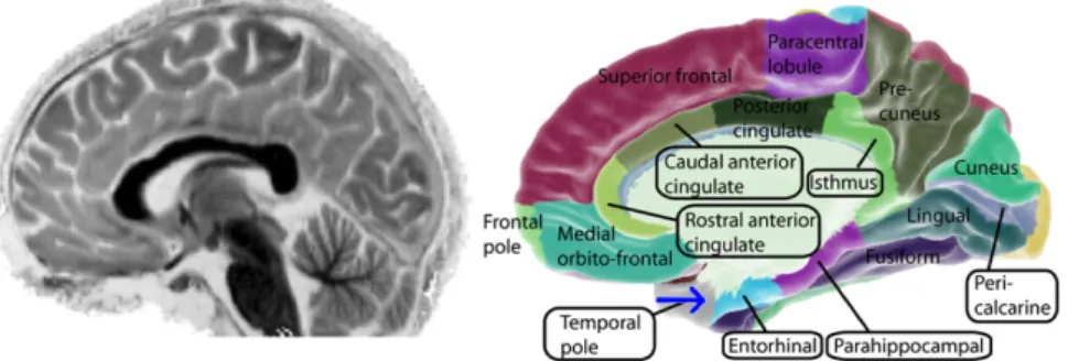
Figure 1.1.1– Left: Integrated MRI image of my brain displaying high spatial

resolution, image produced by 3-T Siemens Magnetom Trio MRI as part of the study by Zeki et al. (2014). Right: Example of anatomical regions of interest over which voxel wise data may be integrated. For each region, a time-series may be constructed (Source: Wikipedia; Hagmann P, Cammoun L, Gigandet X, Meuli R, Honey CJ, et al.).

FMRI Data

If we first consider fMRI data, it is possible to get very high spatial reso-lution, but low resolution in time1. For example, a typical fMRI analysis may capture aroundp= 100,000voxels (the equivalent of a pixel in an image) over a period of several minutes, resulting in aroundT = 200−2000time points. To maintain interpretability this activity is often aggregated into larger regions of interest, an example of possible aggregations is demonstrated in Figure 1.1.1. However, even in the aggregated setting, when one considers the estimation of correlation (a simple measure of variable dependency), the required matrix may have many parameters; a p= 60 dimensional correlation matrix requires the estimation of d =p(p−1)/2 = 1770 parameters. If one further considers that this matrix may change over time, then the problem is still clearly well in the high-dimensional regime.

Traditionally, the estimation of such networks assumes stationarity, i.e. a dependency network for the regions would be estimated assuming that it does not change over time. As such, these stationarity assumptions can affect the level of insight given by the analysis. Increasingly, the aim of studies is not only to find which regions interact with each other, but how this varies over time, or throughout various experimental situations such as performing different tasks. 1_{For a review on statistical analysis of fMRI data, see Lindquist (}₂₀₀₈₎

(22)

Epileptic EEG Trace -200 0 200 -200 0 200 -200 0 200 -200 0 200 -200 0 200 -200 0 200 -200 0 200 -200 0 200 -200 0 200 100 200 300 400 500 600 k=256*t (s) -200 0 200

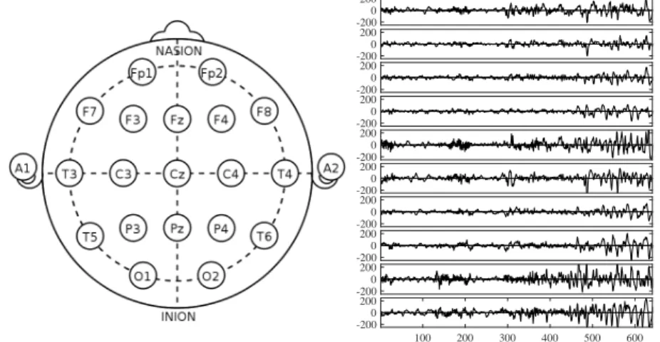
Figure 1.1.2– Left: EEG electrode placement points for the international 10-20

standard. Right: EEG readings for 10 electrodes in the lead up to an epilepsy seizure, see Chapter 6 for more details.

To relax the assumption that the graph is constant over time requires extend-ing the degrees of freedom within the chosen statistical model. Throughout this thesis, and especially in Chapter 3, several approaches to relaxing sta-tionarity assumptions are discussed. In particular, a new type of dynamic graphical model is proposed which can operate in high-dimensions while also detecting changes (or changepoints) across many data-streams. While anal-ysis of fMRI data is not explicitly discussed in this thesis, it is one of the areas where methods developed here may provide great value. Indeed, other researchers are investigating the application of algorithms presented in this thesis to fMRI data, and the similarly motivated work of Monti et al. (2014) and Xu et al. (2013) suggests increasing acceptance of these methodologies in the neuroscience community.

EEG Data

In contrast to fMRI data, EEG sensors provide very high resolution in time at the expense of spatial resolution (see Figure 1.1.2). Recording frequencies of 256Hz are common, which gives rise to an abundance of data, especially when monitoring can take place for prolonged periods of time. For example, epilepsy patients are routinely monitored for days or weeks prior to surgical

(23)

operations. In this data-rich environment, we may not expect to find ourselves in a high-dimensional setting. If we again consider the task of estimating a correlation matrix to describe cross-channel variation we can easily operate in the standard-dimensional setting where T > p2_{. However, if we want to ask}

more questions of the data and describe not just its cross-channel variance, but also its auto-covariance structure, our models very quickly grow in size. For example, a p-dimensional lag h vector auto-regressive (VAR) model will have of orderp2hparameters. If we again consider that these models may have parameters which change over time, then the high-dimensional setting is soon reached.

In Chapter 7, a class of dynamic graphical model is developed that utilises wavelet basis functions. Such models can not only describe cross-covariance, but also how auto-covariance structures change over time. As an example ap-plication, it is demonstrated how these models may be used to characterise EEG activity in the lead up to, and throughout an epilepsy seizure. A par-ticular novelty of the method is that it decomposes dependency structure as a network across a set of different length scales. Therefore, not only is the seizure activity clustered according to seizure, but one can readily see which electrodes appear dependent across a network. Potentially, this may give an indication of how epileptic activity spreads across the brain, which could be of particular value in understanding complex epielpsies where seizure activity is not well localised. If shown to be robust over multiple patients, features such as those proposed here may one day help clinicians improve epilepsy diagnosis and treatment.

1.1.2 Statistical Analysis of Network Traffic

Dynamic graphical models provide a valuable tool not just in the scientific domain, but also to help us understand complex systems in general. Large computer networks, such as the internet, are perhaps one of the most complex and data-rich systems available to study. As computing technology has pro-gressed, it is not only possible to transfer more data across networks, but also monitor this activity itself. Again, in such a data-rich domain, one may ques-tion the need for high-dimensional statistics. For example, if one considers the popular network monitoring protocol NetFlow, it is not uncommon to collect

(24)

hundreds of gigabytes of data. However, when one considers that a large cor-porate network may have thousands of devices attached, it is again plausible that statistical models will have to operate in high-dimensional settings.

Given society’s reliance on computer networks, such systems are increas-ingly being targeted by sophisticated cyber-criminals and other parties. Rather than cause immediate damage and expose themselves to defenders, attackers are increasingly choosing to infiltrate and remain active within a network for extended periods of time. TheseAdvanced Persistent Threats (APT) are hard to detect due to the massive complexity and volume of activity within net-works which can mask the subtle movements of an attacker (Friedberg et al.

2015). TraditionalIntrusion Detection Systems (IDS)operate on a rule-based approach (Patcha et al. 2007), these can react very quickly to detect known threats as long as these correspond to previously modeled and coded patterns. Unfortunately, such hard-coded rules require frequent updating and given their high levels of specificity, such defences are being increasingly bypassed using so-called polymorphic attacks (Fogla et al.2006)2. To counter these rule spec-ification issues, a popular research direction in network anomaly detection is to adopt machine-learning based approaches. Generally speaking, these aim to model different classes of network activity, anomalous or normal, based on some algorithm which is trained on real network data. Two main strands of machine-learning methodologies are employed in the literature:

Discriminative methods: Act to classify network activity as normal or ab-normal based on an explicit labelling of ab-normality, i.e. one has access to some labelled data where the state of the network is known. Sometimes, this may be extended to consider specific types of anomaly, in a task which is known as anomaly identification (Iglesias et al. 2014).

Generative models: Aim to describe an underlying statistical distribution from which observed data might be generated. Anomalous activity can then defined with respect to the estimated distribution (Patcha et al.2007). Many correlation based methods, for exampleprinciple component analysis (PCA), may be seen in this light (Ringberg et al. 2007).

2_{A polymorphic attack is one which is capable of automatically (or easily) adjusting the way} it appears to network monitoring systems, i.e. they do not have a fixed signature.

(25)

No Events

No StartEventsBytes MedianBytes MADBytes SUM Bytes SD Packets MedianPackets MADPackets SUM

Packets SD BP Ratio MedianBP Ratio MADBP Ratio SUM No Events No StartEvents Bytes Median Bytes MAD Bytes SUM Bytes SD Packets Median Packets MAD Packets SUM Packets SD BP Ratio Median BP Ratio MAD BP Ratio SUM | | ( ₁=0) 0 2 4 6 8 10 No Events No StartEventsBytes MedianBytes MAD

Bytes SUMBytes SD Packets MedianPackets MADPackets SUM

Packets SD BP Ratio MedianBP Ratio MADBP Ratio SUM No Events No StartEvents Bytes Median Bytes MAD Bytes SUM Bytes SD Packets Median Packets MAD Packets SUM Packets SD BP Ratio Median BP Ratio MAD BP Ratio SUM | | ( 1=0.1) No_Eve nts No_Sta rtEve nts

Bytes _Me dia n

Bytes _MAD

Bytes _SUM Bytes _SD

Pa cke ts_Me dia n

Pa cke ts_MAD Pa cke ts_SUM Pa cke ts_SD BP_RATIO_Me dia n BP_RATIO_MAD BP_RATIO_SUM BP_RATIO_SD

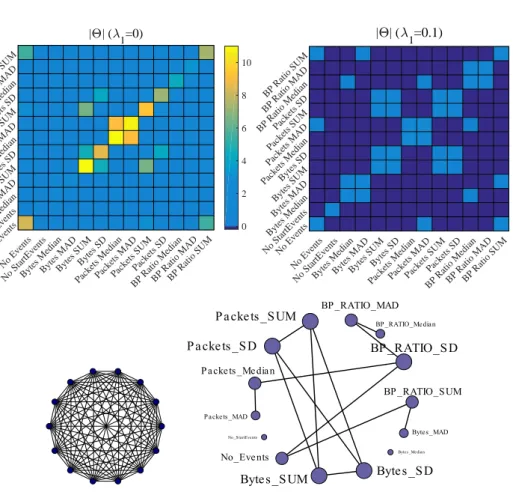
Figure 1.1.3 – Dense (left) and sparse (right) estimates of precision (inverse

covariance) matrices obtained from network traffic features. A graphical mod-elling approach is represented by the sparse model whereby many of the entries in the matrix are zero. The graphical models corresponding to these matrices are given below. The assumption of sparsity clearly provides a more interpretable model and gives increased insight into the data-generation process. The size of the nodes in the estimated graph represent the relative degree (number of edges) associated with each node. A more complete analysis of this data can be found in Section 3.4.2.

To train a discriminative model, we need observations that relate to both network featuresX, which describe traffic flows, and the network state variable Y, which labels whether traffic is anomalous or not. In many situations, we simply don’t know whether the network is in an abnormal state, i.e. we cannot measureY and do not necessarily know whether the network is under attack or not. In the case where we cannot observe the network state directly, a genera-tive approach can prove useful for defining anomalies. Rather than model the conditional distributionP(Y|X), a generative model aims to describe thejoint

(26)

distribution of the network features P(X1, X2, . . . , Xp). Whether the network

is in a normal or anomalous state can be defined relative to the estimated P(X1, X2, . . . , Xp). However, defining and learning a full joint distribution,

as opposed to conditional discriminative, or marginal models is hard due to the inherent complexity of such models. At this stage, a graphical modelling approach can add significant value as they possess the flexibility to model many distributions, but are robust due to their parsimonious construction. As demonstrated in Figure 1.1.3, graphical models enable enhanced interpretation of a dataset by highlighting dependencies between variables. In this case, the graphical structure is derived in a static manner from features derived from computer network traffic. When the graphical model is sparse, that is, there are only a few edges selected, the degrees of freedom in the model are reduced as fewer parameters are needed to specify the distribution. In the application to computer network modelling, the added robustness of graphical models may contribute to reducing the false positive rate of detecting anomalies. The ap-plication of graphical models to modelling computer network data is examined further in Chapter 3.

1.2 Thesis overview

In the rest of this introductory chapter I will give a brief overview of the thesis structure and notation. There are two principle literature reviews con-tained within this thesis. The first, “Regularised Learning” (Chapter 2) pro-vides a relatively mathematical introduction to high-dimensional estimation and convex optimisation; the second, “Locally Stationary Wavelet Processes” is contained in Chapter 5 and relates to more traditional time-series litera-ture. The remaining chapters contain what should be considered as the main contributions of this work.

It is worth remarking at this point that the traditional boundaries be-tween the domains of computer science, statistics, and signal processing are being eroded. Indeed, the developing field of machine-learning may be seen as a result of the inter-disciplinary requirements for modern statistical mod-elling. The work presented throughout this thesis is very much in-line with this convergence of disciplines. For example, the first half focusses on Gauss-ian graphical models, which may be traditionally seen from a statistical and

(27)

1. THESIS OVERVIEW 27

optimisation perspective; the second half is very much born out of statistical signal-processing and the mathematical development of wavelet systems.

A brief summary of chapters is given below:

Chapter 2: Regularised estimation is introduced in the context of M-estimation. The requirement for regularisation is examined in the context of linear re-gression in high-dimensions. Different `p regularisation schemes

along-side optimisation machinery are introduced. Gaussian graphical mod-els (GGM) are defined in the i.i.d. setting and different model-selection schemes discussed. Finally, a theoretical framework for analysing M-estimators in high-dimensions is discussed.

Chapter 3: Dynamic GGM are introduced, recent literature is discussed, and several ways of relaxing stationarity assumptions are compared. Two novel estimators for dynamic graphical models; the group-fused graphical lasso (GFGL), and independently fused graphical lasso (IFGL) are compared. Two algorithms are proposed for estimation of such models. Synthetic experiments are used to highlight the respective properties of the estima-tors. The chapter concludes by considering the applications of dynamic graphical models in genetics and cyber-security.

Chapter 4: A theoretical analysis of the changepoint error with the GFGL estimator is constructed. In standard dimensional settings (p fixed) as-ymptotic changepoint consistency is demonstrated. In high-dimensions the GFGL estimator is discussed in the context of the M-estimation framework introduced in Chapter 2.

Chapter 5: Until this point in the thesis, all models assume that data is independently, but not identically drawn. A class of locally-starionary wavelet (LSW) and Fourier based models are introduced that enable the modelling of auto-covariance structures. Some statistical properties and previously proposed methods for spectral estimation in these models are discussed.

Chapter 6: The potential high-dimensional nature of spectral estimation motivates regularisation of the empirical spectrum. We discuss and im-plement fused smoothers for the spectrum of LSW processes. Such fused estimation is extended to 2-D fields, giving rise to applications in image processing.

(28)

Chapter 7: This chapter translates ideas from Chapter 3 to the estimation of the multivariate LSW spectrum. Synthetic experiments suggest that regularisation can improve estimation performance and recover graphical spectral structure. An application to modelling EEG data throughout epilepsy seizures demonstrates the benefit of regularisation in terms of separating seizure pathways and enabling enhanced interpretation of EEG data.

Chapter 8: The thesis concludes with a discussion of how these methods can be further extended. In particular, it is discussed how one may extend the M-estimation framework of Chapters 2 and 4 to the locally-stationary wavelet setting.

1.3 Notation

Specific notation, i.e. what individual characters mean, may change through-out the thesis, their meaning should thus be considered in the local context. In general, vectors are denoted in bold font and lower case and matrices are bold and upper case. For example:

x= (x1, x2, . . . , xp)> ∈Rp A=    A1,1 · · · A1,q .. . . .. ... Ap,1 · · · Ap,q   ∈R p×q .

Table 1 provides a summary of notation for matrices and vectors. Asymptotic notation is fairly standard. For positive sequences {an}, {bn}; an = O(bn)

means there exists a constant c1 such that an ≤ c1bn. Similarly, an = Ω(bn)

means there is a constant c2 such that an ≥ c2bn. Analogously, for

func-tions we denote f(x) = O(g(x)) to mean |f(x)| ≤ c3|g(x)| for constant

c3. Capitilised non-bold letters are used to describe random variables, if

the variable is multivariate then this is indicated by an arrow. For exam-ple; X~ := (X1, X2, . . . , Xp)> ∼ N(µ,Σ) denotes p variables drawn from a

multivariate normal distribution.

It is worth noting that some probabilistic statements in this thesis may slightly abuse the notation. For example, I may write P[y|X,θ, σ] which

(29)

1. NOTATION 29

actually means what is the probability of obtaining samples yfrom some ran-dom variable Y~ and it’s associated distribution (in this case, this should be parameterised in terms of X,θ, σ).

In much of the thesis the notation can become quite complicated simply due to the number of indexes required. For example, we will deal with quan-tities which may vary as a function of; time, space, scale, or direction, all of which require indexing. Generally, time-indexed quantities will have the nota-tion {x(t)}T

t=1 ={x(1), . . . , x(t), . . . , x(T)}. Super-scripted indices are encased in

brackets to differentiate them from the exponentiation operators. For example, the notation (X(t))−1 refers to the inversion of the matrix X(t) indexed by t.

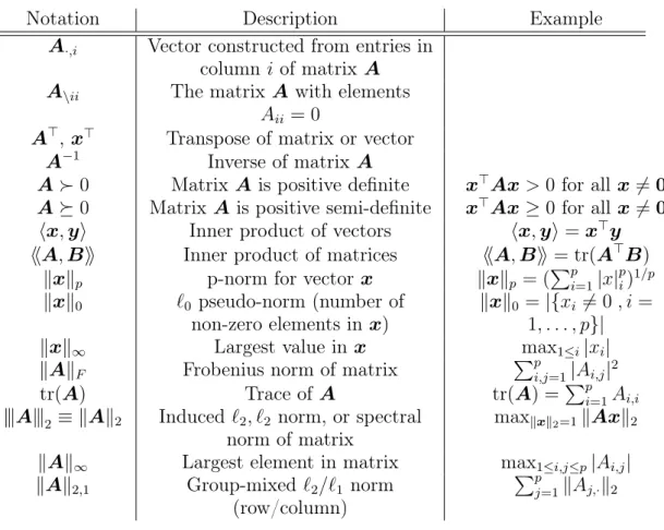
Table 1 – Notation for properties and operations on matrices A ∈ _Rp×p _and

vectorsx∈Rp.

Notation Description Example

A·,i Vector constructed from entries in

columni of matrix A A\ii The matrix Awith elements

Aii = 0

A>, x> Transpose of matrix or vector

A−1 Inverse of matrix A

A0 Matrix Ais positive definite x>Ax >0 for all x6=0

A0 Matrix Ais positive semi-definite x>Ax ≥0 for all x6=0

hx,yi Inner product of vectors hx,yi=x>y

hhA,Bii Inner product of matrices hhA,Bii = tr(A>B)

kxkp p-norm for vector x kxkp = (Pp_i₌₁|x|pi)1/p kxk0 `0 pseudo-norm (number of

non-zero elements inx)

kxk0 =|{xi 6= 0, i=

1, . . . , p}| kxk∞ Largest value in x max1≤i|xi| kAkF Frobenius norm of matrix Pp_i,j₌₁|Ai,j|2

tr(A) Trace of A tr(A) = Pp

i=1Ai,i |||A|||₂ ≡ kAk2 Induced `2, `2 norm, or spectral

norm of matrix

maxkxk2=1kAxk2

kAk∞ Largest element in matrix max1≤i,j≤p|Ai,j| kAk2,1 Group-mixed `2/`1 norm

(row/column)

Pp

j=1kAj,·k2

In Chapters 5,6, 7 it is convenient to use some notation from the signal-processing literature. Primarily, these relate to operations acting on discretely indexed functions f[t], where the square brackets imply that the argument of

(30)

the function is integer valued. Notation for some operations on such functions is summarised in Table 2.

Table 2 – Notation for operations on a discrete function f.

Notation Description Example

f[t] A function supported ont∈S ⊆_Z

f ↑l[k] Up-sampling of f byl and then taking the kth element

f ↑l[k] =

(

f[k/l] k =nl n∈_Z

0 otherwise

f ↓l[k] Downsampling by l and then taking the kth element

f ↓l[k] :=f[lk] (f∗g)[t] Convolution of signal f with filter

g

(f∗g)[t] :=

P∞

(31)

Chapter 2.

Chapter 2 Regularised Estimation

. . . for theories (of equal scope) rendering equally probable our observational data (which, for brevity I shall call equally good at “predicting”), fitting equally well with background knowledge, the simplest is most probably true – Swinburne 1997

From a statistical estimation viewpoint, the significance of a model component or parameter can be viewed in terms of a model selection problem. One may construct a loss function which tells us how well the model fits some data, a lower value of this function implies the model more adequately describes the data. Formally, let us construct this function as L(M,θ,X), where M ∈ M

indexes a model with parameters θ ∈ P(M), and the matrix X relates to some observed data. Additionally, to account for differences in perceived model complexity, one should penalise this with a functionR(M,θ). A morecomplex model should have a larger value of R(·). An optimal identification of model and parameters may then be found through balancing the two terms, such that (2.0.1) ( ˆM ,θˆ) = arg min

M∈M,θ∈P(M)

L(M,θ,X) +R(M,θ).

In statistics such a formulation is referred to as an M-estimator; however, such frameworks are popular across all walks of science (Boyd and Vandenberghe

2004). For example; maximum-likelihood (ML), least-squares (LS) , robust Huber loss, and penalised ML estimators can all be discussed in this context. The principle idea is to suggest a mathematical, and therefore objectively

(32)

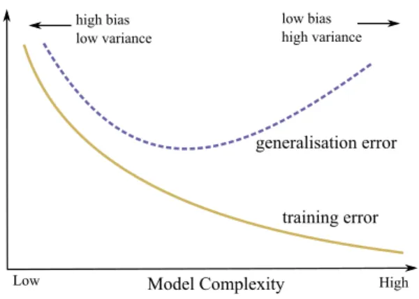
training error generalisation error high bias low variance low bias high variance

Model Complexity High Low

Figure 2.0.1– Generalisation vs training error. Increasing model complexity

may reduce training error, but perform poorly on out-of sample data.

communicable statement to the effect ofOccam’s Razor; given similar model-fit, one should prefer the simpler model (Swinburne1997).

Figure 2.0.1 provides a graphical motivation for the Occam’s Razor in the context of model estimation. If we plot the training and test error of a given set of models (M) with respect to their complexity, we can draw curves cor-responding to those in the figure. The key point to take away is that good performance on training data does not guarantee good performance on the out-of-sample test data. Occam’s Razor and Eq. 2.0.1, therefore suggest we attempt to choose the model with the lowest generalisation error.

Depending on the specification of the functions L(·) and R(·) and associ-ated model/parameter spaces, the problem in (2.0.1) can be either very easy or difficult to solve. Throughout this chapter the motivation for framing sta-tistical estimation problems asconvex1M-estimators is developed. In the next section, we start this discussion in the context of the canonical linear regres-sion model. Specifically, we focus on the high-dimenregres-sional setting where the number of covariates is larger than the number of data-points and traditional estimation methods may fail to identify a model. We discuss why this happens, and how regularisation and formulation of M-estimators can enable model esti-mation, even in the relatively extreme case of high-dimensionality. After this, 1_{Special attention is given to M-estimators (2.0.1) where the constituent functions are convex} as they result in relatively easy optimisation problems. Some properties of convex functions are given in the Appendix A.1.

(33)

2. LINEAR REGRESSION 33

a set of optimisation tools are introduced to help us solve practically solve M-estimation problems; this is followed by an introduction to graphical models. In the final section, a framework for theoretically analysing M-estimators is introduced alongside several key results from the literature.

2.1 Linear Regression

Linear regression is one of the most popular and simple statistical models in use today. Focussing on the predictive task, the model attempts to predict the value of an outcome Y ∈ Y ⊆ _R, conditional on a set of input variables X~ ≡

(X1, . . . , Xp) ∈ X ⊆ Rp. While most of this thesis is not directly concerned

with the task of prediction, but rather descriptive modelling, it is still very important to understand the linear predictive model. In addition to providing a simple introduction to regularised M-estimation, we will later see how the linear model can be adapted for use in dependency and changepoint analysis. In a statistical sense, the end goal of linear regression is to obtain the posterior predictive P[Y = ytest|X~ = xtest,θˆ], where θˆ ∈ Rp are a set of

model parameters estimated on some pre-observed training data. As the name suggests, linear regression assumes the function mapping the feature space to the labels f(θ) : X 7→ Y is linear in nature.

Definition 2.1. Linear Regression Model

The linear regression model has two principle constructions. These are given as the fixed designmodel where the covariates are not random variables

(2.1.1) Y(i) =θ0+ p X j=1 θjx (i) j + (i) _for_i_{= 1}_{, . . . , N ,}

and the random-design model

(2.1.2) Y(i) =θ0+ p X j=1 θjX (i) j + (i) _for_i_{= 1}_{, . . . , N ,}

where (i) _{is a zero-mean noise process (random variable). Additionally, it is}

usually assumed that the noise process is sampled independent, and is identi-cally distributed (i.i.d).

(34)

Typically, one may assume that stochasticity is provided through a Gauss-ian random variable such that(i) i._{∼ N}i.d ₍₀_{, σ}2₎_{. For simplicity, let us consider}

the fixed design case where the intercept θ0 is zero, and the covariates are

centered and measured on the same scale2. For observational pairs (y(i)_,_x(i)₎_,

the linear model (2.1.2) can be written in matrix-vector notation as

y=Xθ+, wherey = (y(1)_{, . . . , y}(N)₎>_∈

RN is theresponse vector, andX = (x(1), . . . ,x(N))>∈ RN×p consists of measured covariates and is known as the design matrix.

Tra-ditionally, one may find estimates for the regression parameters, through either least squares (LS); θˆLS := arg minθPN_i₌₁ky(i)−Xi,·θk2₂ , or if we associate a parameterised model to the errors, viamaximum likelihood estimation (MLE);

ˆ

θMLE := arg maxθP[θ|X,y].

Assuming that we have associated a Gaussian distribution function to our model, the likelihood P(y|X,θ)is given by

P[y|X,θ,Σ] = (2π)−T /2 det(Σ)−1/2

exp

−(y−Xθ)>Σ−1(y−Xθ)/2 . Further, if one assumes errors are i.i.d we can set Σ = σ2I and the above simplifies to

P[y|X,θ, σ] = (2πσ2)−T /2exp[−(2σ2)−1ky−Xθk2 2].

As the name suggests, for the MLE estimator one is required to maximise the above function with respect toθ. For example, say we wish to train the model to a set of observations(y,X)≡(y_train,Xtrain), then one can simply maximise

the likelihood, or equivalently the log-likelihood

{ˆθMLE,σˆ2}:= arg max θ,σ2

logP[y|X,θ, σ2]= arg max

θ,σ2 −N 2 ln(σ 2₎₋ 1 2σ2ky−Xθk 2 2 . Differentiating the log-likelihood and equating to zero leads to the estimators

ˆ

θMLE =(X>X)−1X>y,

2_{This can generally be achieved through}_z-scoring _{the data such that}_y_¯₌_N−1PN

i=1y (i)_{= 0} andˆσ2 j =N−1 PN i=1(x (i) j −x¯j) = 1for allj= 1, . . . , p.

(35)

2. LINEAR REGRESSION 35 ˆ σ2_MLE =1 N(y−X ˆ θMLE)>(y−XˆθMLE).

There are several remarks worth making about the above result:

• The regression parameter estimates obtained through MLE are identical to those obtained viaLeast Squares (LS), ie θˆLS := arg minθky−Xθk22 =

ˆ

θMLE.

• The MLE estimator for the variance differs from the unbiased estimator. Through Cochran’s theorem we have;Nσˆ2

MLE/σ2 ∼ XN2−1 =⇒ E[ˆσMLE2 ] =

σ2₍_N₋₁₎_/N_.

• If (X>X) is singular and cannot be inverted then the MLE problem as above is an ill-posed problem. Additionally, if (X>X) is nearly singular, iedet(X>X)≈0, then the estimates for θˆMLE will be very unstable.

Before proceeding, one may note that the matrix X>X is related (in the random design case) to the empirical covariance estimator for the Gaussian dis-tribution. If the covariates were drawn from a centered multivariate Gaussian distribution such that X~ ∼ N(0,Σ), then the MLE estimator for the covari-ance is given asSˆ =N−1X>X. The covariance matrixSˆ ∝X>X is singular and thus non-invertible when there exists a linear inter-dependency between covariates. Specifically, if there is a linear dependency between columns, i.e.

rank(X>X) < p, then the covariance matrix will be singular and a unique estimate θˆMLE cannot be obtained. With regards to the dimensions p, N we

note; rank(X ∈_Rp×q₎_≤_min(_{p, q}₎_{, and thus} _{rank( ˆ}_S₎_≤ _min(_{p, N}₎3_{. As such,} in the high-dimensional setting where p > N, the covariance matrix becomes singular and the LS and MLE estimates are ill-defined.

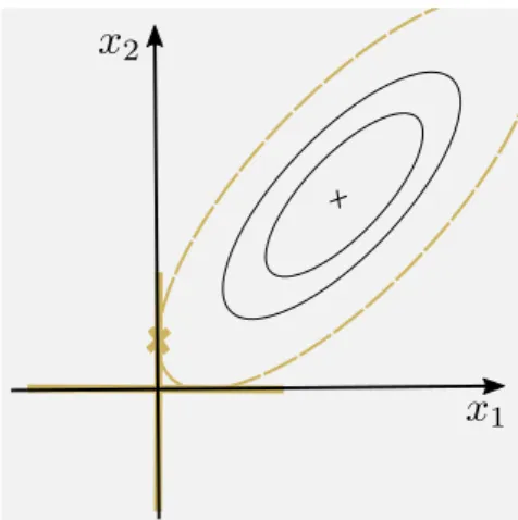
Figure 2.1.1 provides a graphical illustration of how linear dependency between covariates can result in an inability to estimate parameters. While in theN < psetting such singular behaviour is guaranteed, even in settings where N > p, the covariance can almost be singular, i.e. when the angle between x1

and x2 is very small.

It is well known that one can stabilise estimators in the high-dimensional setting by utilising prior knowledge relating to regression parameters. Two traditional approaches for this are discussed in the following sections. The first known asridge-regression aims to shrink the estimates for our parameters 3_{Recall that} _rank(_AB₎_≤_min(rank(_A₎_,_rank(_B₎₎

(36)

Figure 2.1.1 – Linear dependency between covariates provides a problem for estimating the two regression parametersθ1, θ2 as the plane defined by x1,x2 is

no-longer defined.

towards zero. Alternatively, one may performsubset selection and regress onto a small subset of parameters. Interestingly, both of these approaches may be considered in the context of M-estimators, and understood in terms of placing priors on the model parameterisation.

2.1.1 Ridge Regression

One of the simplest priors we can adopt is to assume the parameters are drawn from a Gaussian distribution. For example, one may consider a zero-mean prior with identical varianceσ2

0 along each of thepparameters such that

~

θ ∼ N(0, σ2

0I). If, for simplicity we assume a fixed design matrix, then the

posterior over parameters is now given as

P[θ|X,y] = P[y|X,θ, σ 2_] R P[y|X,θ, σ2_]d_θP[θ], ∝ exp − 1 2σ2 N X i=1 (y(i)−(x(i))>θ !2 exp − 1 2σ₀2 P X j=1 θ_j2 ! . (2.1.3)

Taking the log-posterior; logP[θ|X,y], we arrive at the familiar objective of ridge-regression (Hoerl et al.1970)

LRidge(θ, σ2/σ02) := −ky−Xθk 2 2− σ2 σ2 0 kθk2 2 . (2.1.4)

(37)

Maximising the log-posterior4, or equivalently minimising the negative log-posterior, allows us to gain a unique estimate for the parameter

ˆ

θRidge = arg min

θ∈Rp

[−LRidge(θ, λ)] ,

where the quantity λ = (σ/σ0)2 is known as the regularisation parameter.

Written in this form, the ridge-regression estimator can be directly related to the M-estimator framework of Eq. 2.0.1; consider the loss function L(θ) ≡ ky−Xθk2

2, and complexity penalty R(θ) ≡ λkθk22. Furthermore, since the

ridge regression problem is convex it has a global mimima located at θˆRidge.

Due to this convexity and smoothness, an explicit solution for the posterior mode is easily found by equating the partial derivatives of LRidge(θ) to zero.

The resulting estimate is given as

ˆ

θRidge= (X>X+λI)−1X>y .

Comparing this with the vanilla MLE solution we observe that the use of a Gaussian prior has added a term λI ∈_Rp×p _{to the diagonal of the covariance}

matrix, hence the name ridge regression. Given this additional diagonal term, the solutions are stabilised even in the case whereN p. Unfortunately, this stability comes at the expense of adding a bias into our estimators. Netherthe-less, by adjusting the regularisation strengthλwe now have the ability to move along the bias/variance trade-off curve (Figure 2.0.1). One can interpret the use of a prior as adding extra assumed data to an estimation problem. In this case, adopting the Gaussian prior and likelihood with uniform variance means we are not letting this artificial data lie in any preferred direction. The bias imposed by ridge regression therefore does not preferentially select any parameters, but rather shrinks all the parameters together.

A further interesting way to interpret this prior, is to consider how it re-stricts estimates to what are known as feasible sets. Specifically, if one con-siders the regulariser RRidge(θ, λ) := λkθk22 in conjunction with a certain loss

function, then only solutions within a certain sub-space are allowed. We can see this more clearly by re-writing (2.1.4) as a constrained optimisation prob-lem

4_{Similarly, one may consider the} _{maximum a-posteriori (MAP)} _{estimate. Maximising the} log posterior is equivalent due to the monotonic nature of thelog function.

(38)

Figure 2.1.2 – Diagram of how the ridge regression estimator can be under-stood in terms of an explicitly constrained optimisation problem. Only when the contours of the least squares solution intersect the`2 ball are solutions feasible.

ˆ

θRidge = arg min

θ

ky−Xθk2₂

subject to kθk2

2 ≤l .

(2.1.5)

For a given threshold l, such a formulation is equivalent to the ridge regres-sion in (2.1.4). The appropriate value for l is defined by the regularisation parameter λ in conjunction with the size of the model fit term ky−Xθk2

2.

Figure 2.1.2 presents a graphical representation of both this projection, and other constraints considered in the sequel.

The idea of explicitly constraining estimates via such a norm ball, i.e. such that kθk2

2 ≤l is extremely popular, not just in statistics, but also for general

ill-posed inverse problems (Gockenbach2016). In the next section, projections for different constraint sets that correspond to different prior assumptions are considered and result in new classes of M-estimators.

2.1.2 Subset Selection

A pervasive idea in high-dimensional statistics is that data may lie in some embedded low-dimensional structure or subspace (Meinshausen 2008; Negah-ban et al. 2012). Indeed, as figure 2.1.1 suggests, when the covariance matrix is singular it might be beneficial to reduce the dimensionality of the model.

(39)

For example, in the diagram, rather than regressing onto a plane, we could regress onto a line and choose a subset of features to utilise within the model. A traditional approach to the subset selection problem is to start with no regression parameters (we assume they are inactive and equal to zero) and gradually add them as required. This method known as forward selection starts with an empty set A = {} and then iteratively activates parameters that appear to improve the model. However, we need a way to know when to stop adding parameters, “How far down the model complexity curve in Figure 2.0.1 do we allow our model to go?”

Similarly to the M-estimation idea, a popular way to achieve this is by penalising model fit with a complexity penalty. In particular, some popular penalties are the Akikake Information Criteria (Akaike1973)

AIC(k) := 2k−2L , or the Bayesian Information Criteria (Schwarz 1978)

BIC(k, N) :=k(ln(N)−ln(2π))−2L ,

where L≡ −log(L) is the negative log-likelihood, andk is the number of free parameters required to be estimated, in the forward selection casek =|A|.

Remark 2.1. Complexity penalties in high-dimension

Immediately, one notes that the AIC penalty is not dependent on N as it is derived in the asymptotic setting whereN → ∞. It would immediately seem somewhat inappropriate for use in the high-dimensional setting where we often have relatively small N. On the other hand, whilst BIC does depend onN, this also runs into trouble in the high-dimensional setting. For example, J. Chen et al. (2008) discuss issues of BIC not being able to adapt to high-dimensional model spaces. This is due to an implicit prior P[M] in the formulation of BIC which assigns equal probability for all models M over model space M. For regular problems where the number of parameters k =p is fixed it is well known that BIC is consistent. However, in the high-dimensional setting where the number of covariates included k = |A| varies between models we see that regular BIC assigns probability according to the model class size. For example, consider the class of models S1 with p= 100, but only k =|A| = 1 covariate,

(40)

models with two covariates S2 we find this has size 100 ×99/2. Thus, the

traditional BIC penalty when used to compare models with varying number of covariates assigns much greater probabilities to those with larger active sets. To overcome such inconsistencies J. Chen et al. (2008) suggest an extended BIC definition which actively accounts for the number of active covariates.

All of the above information criteria, including the extended BIC rely on us penalising the likelihood by some quantity proportional to the number of active elements. If we consider the problem in the context of linear regression, we would be required to construct an M-estimator of the form

(2.1.6) θˆA = arg min

θ∈_Rp

ky−Xθk2

2+λ|A(θ)|,

where|A(θ)|=kis the number of active non-zero components at a given point in the parameter space. In machine learning and engineering, the addition of this counting factor is often referred to as an “`0 norm”, although this is not a

norm in the traditional sense5_{. The reason for such abuse of terminology, is that} when one considers aq-norm, often denoted`qof the formkθkq := (P_i|θi|q)1/q.

In the limit q→0 we obtain the`0 normkθk0 ≡ |A(θ)|.

A particularly appealing property of subset selection, is that of sparsity, whereby there exist many zero elements in our estimate, i.e. kˆθk0 ≡ k p.

Unlike the ridge regression setup, wherekθˆRidgek0 =p, when performing subset

selection we have a bias which directs us to preferentially choose some key components. This appeals to us, both in terms of stabilising our estimator by adding bias, but also allowing some form of model interpretation through selection of coefficients. Given the discussion above, the challenge when using subset selection is not necessarily a statistical one, but a computational one.

In the previous section, where we discussed ridge-regression it was noted that the `2 norms led to an overall convex M-estimator as both constituent

functions were convex (see 2.1.5). Unfortunately, this is not the case when one adopts the`0 “norm” (or any `q norm for0≤q <1) as a penalty.

Proposition 2.1. Let x∈_Rp_{, the} _`

q norm kxkq for 0≤q <1 is not convex.

5_{For example,}_k_cx_k

0=kxk0for allc6= 0and thus fails to satisfy the absolute homogeneity

(41)

Figure 2.1.3 – As in the case of ridge-regression, the exact sub-set selection

operator can be understood as an explicitly constrained estimate. In this case the`0 “norm” is confined to the axis, such that the estimator must select one of

the directions, and is hence sparse. For any LS estimate in the grey region, the resultant regularised estimator will be sparse.

Proof. It is sufficient to demonstrate that the epigraph ofkxkqis not a convex

set. See Appendix A.1.

Again, as in the ridge-regression setting, we may consider an explicitly constrained equivalent to (2.1.6) as graphically represented in Figure 2.1.3. Due to the addition of a non-convex function, the overall M-estimator (2.1.6) is also non-convex and it is therefore not guaranteed to have a single minima6. As a result, we are required to perform exhaustive search over the model space. The naive combinatorial cost for checking subsets scales as orderO(2p). Hence, while routines such as forward selection may provide a method to perform this search, they are only feasible for very small problems of size p≈10→40.

In summary, the subset selection methods inspired by BIC can allow for a sparse selection of parameters; however, this comes at a high computational cost due to inherent non-convexity. In the next section, a third penalty func-tion is introduced, which acts as a middle ground between the ridge regulariser and sub-set selection methods. Crucially, this new penalty enables a convex, and thus efficient search, whilst also possessing some parameter selection ca-pabilities.

6_{Note: this can be seen graphically in Figure 2.1.3 where it is not possible to draw a straight} line (or linearly move) from the`0level set on one axis to another.

(42)

2.1.3 Least Absolute Shrinkage and Selection Operator

In this section, possibly one of the most significant methodological ad-vances in modern statistics is introduced. Motivated by the desire to maintain convexity, while keeping the sparsity properties of an estimator, R. Tibshirani (1996) proposed the least absolute shrinkage and selection operator, or lasso estimator7. In practice, the lasso is simply another complexity penalty that can be used in conjunction with the linear-regression least-squares estimator. Written in the unconstrained form, the lasso is defined according to

(2.1.7) θˆLasso:= arg min θ∈_Rp 1 2ky−Xθk 2 2+λkθk1 , where kθk1 := Pp

i=1|θi| is known as the `1 norm. Crucially, unlike ridge

regression, the lasso is capable of selecting parameters; while, unlike exact sub-set selection, it forms a convex problem. The lasso therefore takes a special middle ground in the regularisation hierarchy; the`1 norm is the limiting case

for which an`p norm may be convex (c.f. Prop. 2.1).

Before further discussing the selection properties of the `1 regulariser, it is

worth taking some time to consider how the lasso and`1 regularisation relate,

not just to other ideas in this thesis, but also the wider literature. First of all, given the interesting convex and selection properties of the lasso, there are many many extensions to this method. In line with the M-estimation para-digm, these can generally be seen as incorporating different prior knowledge into the estimation of parameters. For example; the group lasso of M. Yuan et al. (2006), the fused lasso (R. Tibshirani et al. 2005), the elastic net8 (Zou and Hastie2005), andgeneralised lasso9_{(R.J. Tibshirani and J. Taylor} ₂₀₁₁_),

all enable a practitioner to incorporate prior knowledge into an estimate. Fur-thermore, the development of the lasso, and more general shrinkage estimators is closely tied with work in signal processing where the problem (2.1.7) is often referred to asbasis pursuit denoising problem (BPDN) (Candes et al. 2005)10_.

7_{The original lasso paper by Tibshirani had (according to Google) approximately 9500} cita-tions in 2014, today, it has over 20,000.

8_{A linear combination of}_`

1 and`2 penalties.

9_{The penalty is constructed of a linearly transformed parameter, i.e.} _k_{T θ}_k 1. 10_{One can interpret the lasso problem as attempting to find a sparse (in the}_`

1 sense) set of

(43)

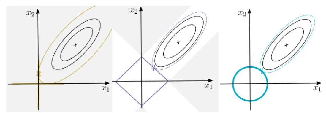
Figure 2.1.4– Comparison ofp-norm constraints, forp= 0,1,2corresponding

to exact, lasso and ridge regression respectively. Shaded areas represent areas in which if the MLE/LS estimate falls then only one of the two parameters(x1, x2)

will be selected. The`2 norm does not select an explicit sparse subspace. In the `0 case we assume that the constraint level is set tokxk0≤1.

In Chapter 5, these relationships are explored in more detail, in the context of wavelet denoising (D. L. Donoho et al. 1995; D. Donoho 1995; D. Donoho et al. 1994) and non-parametric smoothing (R.J. Tibshirani 2014). As hinted at earlier in the introduction, one of the main aims of this chapter is to motivate the formulation of convex M-estimators. Additionally, we note that the prop-erty of sparsity is desirable from an interpretability point of view. The lasso estimator provides the canonical M-estimator which possesses both convexity and sparsity properties. More importantly for this thesis, the lasso also has a counterpart which can be used for dependency analysis, known as the graph-ical lasso (Banerjee et al. 2008; Friedman, Hastie, and R. Tibshirani 2008). This is further discussed in Section 2.3.5; however, has direct parallels with the ideas introduced here.

Let us now further consider the properties of the lasso estimator. As with the ridge-regression, the problem (2.1.7) can be written in an explicitly con-strained form:

ˆ

θLasso: = arg min

θ∈_Rp 1 2ky−Xθk 2 2 subject to kθk1 ≤l . (2.1.8)

Again, as in (2.1.5) given (y,X) there is a one-one mapping between the threshold l and regularisation parameter λ. It seems then, that the lasso can

(44)

also be interpreted as constraining an estimator through projection onto a norm ball. In the case of the lasso we have the constraint that the optimal pointθˆ∗, should lie in a feasible sub-level set

(2.1.9) C`1 ={θ∈dom(k · k1)| kθk1 ≤l},

where θˆ∗ ∈ C ⊆ _Rp_{. At first it is not clear how such a restriction enforces}

sparsity within the estimates. Again, such a property is perhaps best demon-strated geometrically. Figure 2.1.4 demonstrates the contrasting shapes of the constraint sets provided by the differentp-norms considered so far. In both the `0 and `1 cases, corresponding to subset and lasso selection respectively, it is

quite clear that the norm is not smooth at the boundaries between quadrants. This lack of smoothness mandates that within large regions of the parameter space, estimates will be constrained simply to a point. Since the example in Figure 2.1.4 considers a model with two parameters, one of the parameters will be shrunk exactly to zero, hence we obtain a sparse estimate.

The convexity of both the lasso and ridge regression (`1, `2) constraints is

evident from Figure 2.1.4; one can easily see how it is possible to linearly move from point to point within the sets. As previously mentioned, in the exact-selection `0 case (2.1.6), we find the function f(x) = kxk0 is not convex; the

sub-level set for the`0 function the set only contains entries at the axis where

x1 orx2 are zero. However, while the`1 norm is convex, it is not continuously

differentiable and possesses a discontinuity at the origin. In the next sections, an extended calculus which can deal with discontinuous functions is introduced. The enables us to minimise the lasso objective and further assess the behaviour of the estimator.

2.1.4 Optimality Conditions for the Lasso

The lasso allows us to encourage some level of sparsity and selectivity within our model parameterisation whilst maintaining convexity. However, unlike in the ridge-regression or least squares problems, the lasso problem involves a non-smooth kxk1 penalty term. There is a clear discontinuity at the origin,

(45)

Figure 2.1.5 – The lasso regulariser term R(x) = λkxk₁. Note, the gradient

is classically well defined for all regions except the origin where there is a clear discontinuity.

we introduce a concept known as a subdifferential which provides a value, or a set of values, for the gradient at all points:

Definition 2.2. Let f ∈conv(V), and V∗ _{be the dual space of} _V_{. The vector} ψ∈ V∗ _{is called a} _subgradient _of _f _at _x_{∈ V} _if

(2.1.10) f(y)≥f(x) +hy−x,ψi for ally∈ V .

The subdifferential is defined as the set of subgradients at x. For a convex function this is given as the closed interval∂f(x) = [a,b]with one-sided limits:

(2.1.11) a= lim y→x− f(y)−f(x) y−x , b= limy→x+ f(y)−f(x) y−x .

In the above case, if the limits from both sides are equal then the subdiffer-ential contains only a single entry and the function is classically differentiable at that point. Crucially, we now have the ability to deal with discontinuous functions through the notion of the subdifferential set ∂f(x) ∈ [a,b]. For example, the subdifferential of the `1 norm over x∈Rp is given as:

(2.1.12) ∂kxk1 ∈    {sign(xi)} if xi 6= 0 [−1,1] if xi = 0 , fori= 1, . . . , p.

The minima of the convex lasso problem can now be found by considering that the gradient evaluated an optimal point θ∗ must be zero

(46)

0 ∈ ∂L(θ, λ)|θ=θ∗ = ∇(1 2ky−Xθk 2 2) +λ∂kxk1 = −X>y+X>Xθ+λ∂kxk1 , (2.1.13)

Rearranging, we arrive at the so-calledKarush-Kuhn-Tucker (KKT) optimal-ity conditions for the lasso

(2.1.14) X>(y−Xθ∗)∈λ∂kxk1 .

Note that there is no equality in the above statement, as even though the lasso problem (2.1.7) is convex, it is not always strictly convex, this is espcially the case when p N. Generally, further analysis of the curvature of the loss function is required in order to show estimation stability. Further discussion of this is provided in Sec. 2.4. A requirement for strict convexity means the standard lasso problem saturates and can only select up to N variables (Bühlmann et al. 2011). If one wishes to include more variables, it is possible to use extensions such as the elastic-net (Zou and Hastie 2005) which utilise a combination of`2 and `1 penalties.

Due to the importance of the lasso estimator and`1regularisation

through-out the thesis, it is useful to discuss further properties of the estimators. In the next section, we discuss the application of lasso in the simple orthonormal design case, where closed form solutions are available. In the general case one requires an optimisation scheme which can deal with non-smooth functions. Some machinery for optimising such functions is introduced in Sec. 2.2.1.

2.1.5 Analysis in the Orthonormal Design Case (a

rela-tion to thresholding)

An intuitive understanding of the lasso is gained if one considers the or-thonormal case whereX>X =I ∈_Rp×p_{. Clearly, in this case} _rank(_X>

X) =

p, and thus we are not restricted by the stability considerations that we faced previously when dealing with design matrices with p > N. It is also worth

(47)

Figure 2.1.6– Comparison of soft and hard thresholding operators,

correspond-ing respectively to the`1 and `0 proximity operators. The dashed line indicates

the shrinkage/selection of the adaptive lasso.

remarking that the lasso problem with an orthogonal design is directly related to the problem of denoising via wavelet shrinkage (see Chapters 5,6).

Proceeding to set X>X = I in Eq. 2.1.13, gives us the KKT conditions in the orthonormal case:

θ =X>y−λ∂kxk1 .

In the orthogonal situation the least squares solution is given as θˆLS =X>y.

Given that the subdifferential is defined at the individual parameter level, then for i= 1, . . . , p , for the active components (i.e θi 6= 0) we now have

θi = ˆθ

(i)

LS−λsign(θi).

Furthermore; if θi <0, then θˆ(_LSi) <−λ; and if θi >0, thenθˆ_LS(i) > λ. Finally, in

the case|θˆ(_LSi)|> λ we have sign(θi) = sign(ˆθ(_LSi)); we thus obtain

θi = sign(ˆθ

(i) LS)(|θˆ

(i)

LS| −λ).

In the alternate case, where |θˆi

LS| < λ, we have, from the subgradient; θi =

λ[−1,1]−θˆi

LS= 0. Gathering the two cases together we find

ˆ θ(_Lassoi) =    0 if |θˆ(_LSi)|< λ ˆ θ(_LSi)−λsign(ˆθ_LS(i)) if |θˆ(_LSi)|> λ .

(48)

The above can be re-written as below and is known as the soft-thresholding operator

(2.1.15) θˆLasso= soft(ˆθLS;λ) := sign(ˆθ (i)

LS)max(|θˆ (i)

LS| −λ,0),

for each element i= 1, . . . , p. From the above, the solution of the lasso in the orthonormal case acts as a thresholding operator on the ordinary least squares solution.

Figure 2.1.6 demonstrates the effect of this operator in comparison to that of the hard-thresholding operator which arises in the `0 penalisation case.

The lasso solution not only selects certain parameters when |θˆ_LS(i)| < λ, but when parameters are non-zero this adds a shrinkage bias with respect to the LS estimates. The bias associated with shrinkage is often undesirable. For example, Bühlmann et al. (2011) discuss how this may lead the lasso to over-estimate the number of true active covariates.

2.2 Convex Optimisation

Whilst we have discussed solutions of the lasso in the orthonormal setting, methods to solve the general design case have not been discussed. In this section a modified approach to gradient descent is introduced that enables us to deal with non-smooth objectives. Additionally, a method for splitting objective functions up into simpler problems is introduced. For more details and a complete review on convex optimisation, the texts by Boyd, Parikh, et al. (2011) and Nesterov (2007) and Boyd and Vandenberghe (2004) are recommended.

2.2.1 Proximal gradient descent

In conventional (smooth) optimisation problems the canonical approach to obtaining minima is via gradient descent type algorithms. Extending gradi-ent descgradi-ent methods to cope with non-smooth objectives requires re-thinking how we step through parameter space when faced with discontinuous func-tions. One such method, known as proximal gradient descent revolves around minimising a surrogate function known as theMoreau envelope.

(49)

2. CONVEX OPTIMISATION 49

Definition 2.3. The Moreau envelopeor Moreau-Yoshida regularisationMλf

of the function λf is defined as:

(2.2.1) Mλf(v) = inf x f(x) + 1 2λkx−vk 2 2 .

The Moreau envelope can be interpreted as a smoothed form off that has domaindom(Mλf)∈Rp and is continuously differentiable even when f is not.

Furthermore, the sets of minimisers for f and Mf are the same (see Nesterov

(2005)). This property can be useful for generalising gradient descent methods to non-smooth objectives, such as those found in the lasso.

Proposition 2.2. Geometric Moreau

Let f be convex and closed on the Hilbert space V =H, with dual V∗ ₌_H_. Then for every z ∈ H there is a unique decomposition

(2.2.2) z = ˆx+ψ withψ∈∂f(ˆx),

and the unique xˆ in this decomposition can be computed with the proximal operator:

(2.2.3) prox_f(z) := arg min

x∈H

1

2kx−zk

2

H+f(x) .

Proof. See Parikh et al. (2013) and Rockafellar (1970).

Essentially, this result provides us with a way to move along our function by stepping in the direction given by the gradient (sub-gradient) ψ. The Moreau envelope can now be related to the proximal operator, as the proximal operator returns the minimal value ofMλf, such that

Mf(x) = f(proxf(x)) +

1

2kx−proxf(x)k

2 2 .

Proposition 2.3. Let zˆ be a fixed point, such that; zˆ = prox_f(ˆz). The min-imiser of the functional f is thus zˆ.

Proof. This is a consequence of Moreau’s theorem 2.2.2, where we have zˆ ∈