Bayesian inference for continuous-time step-and-turn movement models

(1)

Bayesian inference for continuous-time

step-and-turn movement models

Alison Parton

School of Mathematics and Statistics

Faculty of Science

The University of Sheffield

This dissertation is submitted for the degree of

Doctor of Philosophy

(2)

(3)

Declaration

I hereby declare that except where specific reference is made to the work of others, the contents of this thesis are original and have not been submitted in whole or in part for consideration for any other degree or qualification in this, or any other university. This thesis is my own work and contains nothing which is the outcome of work done in collaboration with others, except as specified in the text and the following acknowledgements.

Alison Parton April 2018

(4)

(5)

Acknowledgements

I would like to thank the School of Mathematics and Statistics at the University of Sheffield for funding this PhD. Thanks to Professors Jeremy Oakley and Caitlin Buck for your inspiration and encouragement in pursuing an academic career. Thank you so much to my supervisor Professor Paul Blackwell for your expertise, guidance and infinite patience—I’ve thoroughly enjoyed my time skulking at your office door.

Chap. 2 features an extension to the edited contribution in the review Patterson et al. (2017). Thank you to my co-authors (Toby Patterson, Roland Langrock, Len Thomas and Ruth King), David Borchers and two anonymous referees on their useful feedback on this material. A proportion of the work in Chaps. 3 and 5 is an extended description of Parton et al. (2017), in particular the reindeer example of Sect. 5.3. Thank you to my co-author, Anna Skarin, for providing the reindeer data and feedback on this approach. The model framework and elk example featured in Chap. 4 are an expanded version of Parton and Blackwell (2017). Thanks to Théo Michelot and two anonymous referees for their comments on this work. I am grateful to the many staff and students within the department and wider university who have supported me in pub locations across the city. Thanks to the Old House and the Notty for all the pies we have consumed and the f.r.i.e.n.d.s who forgive my empty promises of top-tier keg beer offerings.

Thank you to Adam for your constant support and (almost) never-ending ability to appear engrossed in yet another talk rehearsal.

(6)

(7)

Abstract

This thesis concerns the statistical modelling of animal movement paths given observed GPS locations. With observations being in discrete time, mechanistic models of movement are often formulated as such. This popularity remains despite an inability to compare analyses through scale invariance and common problems handling irregularly timed observations. A natural solution is to formulate in continuous time, yet uptake of this has been slow, often excused by a difficulty in interpreting the ‘instantaneous’ parameters associated with a continuous-time model.

The aim here was to bolster usage by developing a continuous-time model with interpretable parameters, similar to those of popular discrete-time models that use turning angles and step lengths to describe the movement process. Movement is defined by a continuous-time, joint bearing and speed process, the parameters of which are dependent on a continuous-time behavioural switching process, thus creating a flexible class of movement models. Further, we allow for the observed locations derived from this process to have unknown error. Markov chain Monte Carlo inference is presented for parameters given irregular, noisy observations. The approach involves augmenting the observed locations with a reconstruction of the underlying continuous-time process.

Example implementations showcasing this method are given featuring simulated and real datasets. Data from elk (Cervus elaphus), which have previously been modelled in discrete time, demonstrate the interpretable nature of the model, finding clear differences in behaviour over time and insights into short-term behaviour that could not have been obtained in discrete time. Observations from reindeer (Rangifer tarandus) reveal the effect observation error has on the identification of large turning angles—a feature often inferred in discrete-time modelling. Scalability to realistically large datasets is shown for lesser black-backed gull (Larus fuscus) data.

(8)

(9)

List of figures

1.1 Parametrisation of movement in the discrete-time step-and-turn model . . . 4

1.2 Structure of a state-space model . . . 8

1.3 Structure of a hidden Markov model . . . 9

3.1 Single state simulated paths . . . 35

3.2 Observations augmented with a single state refined path . . . 36

3.3 DAG of single behaviour movement model . . . 37

3.4 Section of the full single state refined path to update over. . . 41

3.5 Simulated path and observations (independent step model) . . . 51

3.6 Initial path locations (independent step model) . . . 53

3.7 Initial bearings and speeds (independent step model) . . . 54

3.8 Sampled bearing variance against mean speed (independent step model) . . 56

3.9 Sampled speed mean against variance (independent step model) . . . 57

3.10 Posterior credible intervals of parameters (independent step model) . . . 59

3.11 Detailed path reconstructions (independent step model) . . . 61

3.12 Full path reconstructions (independent step model) . . . 62

3.13 Simulated path and observations (correlated step model) . . . 63

3.14 Initial path locations (correlated step model) . . . 65

3.15 Initial bearings and speeds (correlated step model) . . . 66

3.16 Sampled bearing variance against mean speed (correlated step model) . . . 67

3.17 Sampled speed correlation against variance (correlated step model) . . . 68

3.18 Posterior credible intervals of parameters (correlated step model) . . . 70

3.19 Full path reconstructions (correlated step model) . . . 73

3.20 Detailed path reconstructions (correlated step model) . . . 74

4.1 Multistate simulated bearings and speeds . . . 79

4.2 Multistate simulated locations . . . 80

(12)

xii List of figures

4.4 DAG of multistate model . . . 83

4.5 Section of the full multistate refined path to update over. . . 88

4.6 Simulated path and observations (two-state simulation) . . . 95

4.7 Simulated bearings, speeds and behaviours (two-state simulation) . . . 96

4.8 Initial configuration of bearings, speeds and behaviours (two-state simulation) 98 4.9 Sampled behavioural parameters (two-state simulation) . . . 99

4.10 Sampled movement parameters (two-state simulation) . . . 100

4.11 Parameter kernel density estimates (two-state simulation) . . . 101

4.12 Short-term speed variance kernel density estimates (two-state simulation) . 103 4.13 Posterior behavioural state probabilities (two-state simulation) . . . 104

4.14 Path reconstruction with high certainty (two-state simulation) . . . 106

4.15 Uncertain path reconstruction (two-state simulation) . . . 107

4.16 Path reconstruction with behavioural misclassification (two-state simulation) 108 4.17 Observations (two state elk) . . . 110

4.18 Initial path (two-state elk) . . . 112

4.19 Samples of the behavioural parameters (two-state elk) . . . 113

4.20 Samples of the movement parameters (two-state elk) . . . 115

4.21 Probability of residency in behavioural states (two-state elk) . . . 117

4.22 Behavioural residency time density (two-state elk) . . . 118

4.23 Path reconstructions (two-state elk) . . . 119

4.24 Detailed section of path reconstructions (two-state elk) . . . 120

5.1 Noisy observations augmented with a single state refined path . . . 124

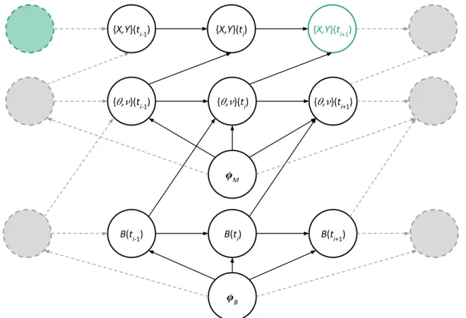
5.2 DAG of movement model with error . . . 125

5.3 Section of the refined path to update over when observation error is present. 127 5.4 Observations (noisy single state reindeer) . . . 130

5.5 Samples of the movement parameters (noisy single state reindeer) . . . 133

5.6 Posterior densities of the movement parameters (noisy single state reindeer) 134 5.7 Path reconstructions (noisy single state reindeer) . . . 136

5.8 Sampled observation error (noisy single state reindeer) . . . 137

5.9 Detailed path reconstructions (noisy single state reindeer) . . . 138

5.10 Observations (noisy two-state gull) . . . 140

5.11 Samples of the behavioural parameters (noisy two-state gull) . . . 142

5.12 Posterior behavioural state probabilities (noisy two-state gull) . . . 143

5.13 Samples of the movement parameters (noisy two-state gull) . . . 144

5.14 Error variance density (noisy two-state gull) . . . 146

(13)

List of figures xiii

5.16 Samples of the movement parameters (1) (observation error simulation) . . 150

5.17 Samples of the movement parameters (2) (observation error simulation) . . 151

5.18 Posterior density of the movement parameters (observation error simulation) 152 5.19 Posterior density of the movement parameters (observation error simulation) 153 5.20 Path reconstructions (observation error simulation) . . . 156

5.21 True location reconstruction with small error (observation error simulation) 158 5.22 True location reconstruction with large error (1) (observation error simulation)159 5.23 True location reconstruction with large error (2) (observation error simulation)161 5.24 Section of the refined path to update over with correlated observation error . 163 6.1 Observed heterogeneity in reindeer movement . . . 170

6.2 Low signal-to-noise observations of reindeer movement . . . 170

6.3 Returns to the same site in gull movement . . . 175

B.1 Posterior densities of movement parameters (independent step model) . . . 191

B.2 Movement parameter trace (independent step model) . . . 192

B.3 Movement parameter ACF (independent step model) . . . 193

B.4 Speed correlation trace at sampling time scale (correlated step model) . . . 194

B.5 Movement parameter trace (correlated step model) . . . 195

B.6 Movement parameter ACF (corr step model) . . . 196

B.7 Posterior densities of movement parameters (correlated step model) . . . . 197

B.8 Initial path (two-state simulation) . . . 198

B.9 Parameter sample trace (two state simulation) . . . 199

B.10 Short-term speed variance sample trace (two-state simulation) . . . 200

B.11 Initial path as bearings and speeds (two-state elk) . . . 201

B.12 Parameter trace (two-state elk) . . . 202

B.13 Posterior densities of parameters (two-state elk) . . . 203

B.14 Initial bearing and speeds (noisy single state reindeer) . . . 204

B.15 Parameter trace (noisy single state reindeer) . . . 205

B.16 Parameter ACF (noisy single state reindeer) . . . 206

B.17 Behaviour parameter trace (noisy two-state gull) . . . 207

B.18 Posterior densities of behaviour parameters (noisy two-state gull) . . . 208

B.19 Movement parameter trace (noisy two-state gull) . . . 209

B.20 Posterior densities of movement parameters (noisy two-state gull) . . . 210

B.21 Sample trace of the movement parameters (observation error simulation) . . 211 B.22 Posterior distribution of movement parameters (observation error simulation) 212

(14)

(15)

List of tables

3.1 Initial parameters, perturbation variances and acceptance rates (independent step model) . . . 52 3.2 Posterior credible intervals of movement parameters (independent step model) 60 3.3 Initial parameters, perturbation variances and acceptance rates (correlated

step model) . . . 64 3.4 Posterior credible intervals of movement parameters (correlated step model) 71 4.1 Posterior credible intervals of behavioural parameters (two-state simulation) 100 4.2 Posterior credible intervals of movement parameters (two-state simulation) 103 4.3 Posterior credible intervals of behavioural parameters (two-state elk) . . . . 114 4.4 Posterior credible intervals of movement parameters (two-state elk) . . . . 116 5.1 Posterior credible intervals of parameters (noisy single state reindeer) . . . 135 5.2 Posterior credible intervals of behavioural parameters (noisy two-state gull) 142 5.3 Posterior credible intervals of movement parameters (noisy two-state gull) . 145 5.4 Posterior credible intervals of the observation error variance (noisy two-state

gull) . . . 145 5.5 Posterior credible intervals of parameters (observation error simulation) . . 154 5.6 Posterior credible intervals of parameters (observation error simulation) . . 155

(16)

(17)

List of Algorithms

1 Simulating single state movement. . . 34

2 Sample conditional bearing process parameter . . . 39

3 Sample conditional distance process parameters . . . 40

4 Simulate bearing proposal . . . 42

5 Simulate step proposal . . . 44

6 Correlated step bridge distribution . . . 49

7 Simulating multistate movement. . . 81

(18)

(19)

Nomenclature

List of Abbreviations

ACF Autocorrelation function BB Brownian bridge

BM Brownian motion BRW Biased random walk CRW Correlated random walk

CTMC Continuous-time Markov chain DAG Directed acyclic graph

DTMC Discrete-time Markov chain ESS Effective sample size

GPS Global Positioning System HMM Hidden Markov model

iid Independent and identically distributed MCMC Markov chain Monte Carlo

MH Metropolis-Hastings OU Ornstein-Uhlenbeck

(20)

xx Nomenclature

PMCMC Particle Markov chain Monte Carlo SDE Stochastic differential equation

SSM State-space model SVF Semivariance function VHF Very high frequency

(21)

Chapter 1 Introduction

Movement is fundamental to an animal’s survival, yet the details of such a process are almost unknown. Wildlife trajectories are difficult to interpret, being a complex, noisy mixture of decisions that regularly exhibit randomness, non-linearity, and high spatial and temporal correlations. Internal behavioural states, physical constraints and memory regulate movement, whilst encounters with the environment, such as landscape, weather and other individuals, influence this decision-making process (Cagnacci et al., 2010).

Advances in tracking technologies have allowed data collection on individual animal move-ment at increasing precision and frequency. This has led the way for growth of research into movement ecology, concerned with questions of patterns in animal movements. Phenomena of interest include: the underlying mechanisms and causes for animals to move through space, the constraints affecting this movement (including internal and external influencing factors), and how these movements shape the animal’s overall ecology. Although the focus here will be on the analysis of trajectories of individual animals, such research has the potential to impact other facets of movement ecology, such as: home-range analysis, resource use/selection and group movement.

The ability to collect observations at increased sampling frequencies has particularly steered research to study movement in the short-term, motivating the study of behaviours. Although real movement behaviour is highly complex and dynamic, much of the research in this area assumes that movement is driven by switches between ‘behavioural modes’ that allow for differing phases of the trajectory. The growing interest in this area involves identifying these “statistically detectable signatures” (Fleming et al., 2014a). Driving questions include the number of behavioural modes present in a trajectory, when/how often transitions between

(22)

2 Introduction

these modes occur, and the characterisation of the underlying movement each behaviour represents.

Although the yearly number of publications on animal movement has doubled over the last 10 years, this remains dominated by the documentation of studies rather than addressing ecological questions (Holyoak et al., 2008). Large datasets and limiting computational power lead to a constant trade-off between models that are ecologically realistic and those that are feasible to implement. Overly complex models may capture the realism of individual movement but lack the machinery required to fit them and remain inaccessible to ecologists. In contrast, simplistic models are often employed in an attempt to avoid these complexities, ignoring the directionality and correlation present in movement (Brownian motion and Levy flights, for example (Pyke, 2015)). These single parameter models cannot describe the complex nature of movement, yet often make strong conclusions about it. There is a requirement for approaches that are able to capture enough realism of trajectories to address ecological questions on movement, whilst maintaining statistical robustness and interpretability.

1.1 Movement data

Movement data generally consists of location fixes of an animal (or group of animals) over a sequence of discrete points in time. For land-based animals such fixes are in the two-dimensional horizontal plane. Observations of aerial and marine animals are commonly collected in either the horizontal plane or the one-dimensional vertical direction, and only rarely in the full three dimensions. A variety of collection methods exist for movement observations, but Global Positioning System (GPS) will be the focus of the following work as it is the predominant collection method for modern studies. Historically, collection was by very high frequency (VHF) radio (Cagnacci et al., 2010; Hebblewhite and Haydon, 2010), and other collection methods for movement (direct or indirect) such as camera traps, accelerometers and magnetometers exist, but are not discussed further here (see evaluations in Cooke et al. (2004, 2013); Rutz and Hays (2009); Wilmers et al. (2015)).

The sampling scheme of movement observations vary considerably from sub-second to multiple days based on the particular focus of study and battery size/life. Sampling frequency affects the questions explorable from a set of observations; if migration is of interest then daily observations over multiple years may be sufficient whilst if foraging periods are of concern then observations may need to be at the short scale, such as minutes. It is important

(23)

1.1 Movement data 3

that the sampling scheme is at a meaningful temporal scale with regards the animal dynamics being explored.

The common feature that sampling schemes are often irregular complicates statistical mod-elling of animal movement. A number of observations may be missing from the regular sequence of times either randomly or with structure through temporal or locational con-straints. Small irregularities in sampling times are introduced when a measuring device attempts regular fixes but is delayed through either sensor, battery or memory limitations. Structured irregularities in observations may provide information on movement; such as the times at which seals are underwater making GPS fixes impossible.

A feature of movement data is the autocorrelation in the observed process—an animal’s location in the near future will depend heavily on its current location. At high sampling frequencies this correlation is particularly strong and needs consideration when modelling movement (Cushman, 2010). It is undesirable to apply the informal, ad-hoc methods of some studies which remove observations until autocorrelation is assumed negligible (Nations and Anderson-Sprecher, 2006) or inflate parameter error ranges post-analysis (Fieberg et al., 2010); instead we believe robust techniques that incorporate correlation should be favoured. Telemetry observations introduce spatial and temporal error in the true location of the animal. Due to the nature of GPS technology, the level of observation error is closely linked to the animal’s environment and this introduces autocorrelation in the error process over time. For GPS devices, such errors are considered to be small at 10–28 m (Frair et al., 2010), but the level of effect this has on inference will depend on the movement scale of the animal in question. Further, the error structures obtained from some technologies (e.g. Argos, see McClintock et al. (2015)) are known to be complex and non-Gaussian.

After the collection of animal locations, movement modelling may be carried out based on a number of movement metrics (see e.g. Calenge et al. (2009)), including;

• the raw locations themselves,

• the increments in locations (as displacement or ‘velocity’),

• the Euclidean distances between two consecutive locations (‘steps’), • the compass direction between two consecutive locations (‘bearings’), and • the change in direction between three consecutive locations (‘turns’).

Note that when considering steps and either bearings or turns together, such a bivariate process (given an initial location) defines the raw location process. This alternative parametrisation of movement has been modelled since the early days of telemetry (Marsh and Jones, 1988; Siniff

(24)

4 Introduction

and Jessen, 1969) and has proved popular, described as the “intuitive approach” (McClintock et al., 2014). The development of modelling animal movements based on this metric is therefore outlined in the following section.

1.2 Discrete-time step-and-turn movement

Probably the earliest example of an approach to movement modelling that has become well-established by ecologists is the step-and-turn model. The characterisation of movement into a bivariate time series of turning angles and steps lengths was first used by Siniff and Jessen (1969) to gain insight into the movement of hares and foxes. The turning angle,φ, is the

angle between three consecutive observed locations and the step length,r, is the straight line distance between two consecutive observed locations—Fig. 1.1 shows this parametrisation. Siniff and Jessen (1969), and later models building upon this, propose parametric distributions for these two variables so that the likelihood given observed locations{Z₁, . . . ,Z_M}is

p {Z₁, . . . ,Z_M} |Ω= M−2

∏

i=1 Φ φi|Ωφ M−1

∏

i=1 R r_i|Ωr , (1.1)

whereΦandRdenote the parametric distributions of the turning angles and steps,

respec-tively, andΩis the set of parameters defining such distributions. Note that for a set ofM

observed locations, there areM−1 derived step lengths andM−2 derived turning angles. Statistical inference is then concerned with learning about the parametersΩ, given

obser-vations{Z₁, . . . ,Z_M}. Note from Eq. 1.1 that there is an assumption that the step and turn processes are independent from one another.

The distance an animal can travel between two locations is constrained to be positive, and so it is assumed that the step length,r, arises from some positive parametric distribution;

ϕ

r

Observed location

Fig. 1.1 Parametrisation of movement in the discrete-time step-and-turn model. Define movement between observed locations by the turning angle,φ, and the step length,r.

(25)

1.2 Discrete-time step-and-turn movement 5

common choices for Rin Eq. 1.1 include the gamma and Weibull distributions. The turn that an animal can achieve between two points in time is unconstrained, but is constrained to [−π,π]when observed. The turns, φ, are therefore assumed to arise from a wrapped

distribution with such boundaries; options forΦin Eq. 1.1 include the von Mises (closely

related to the wrapped normal) and the wrapped Cauchy distributions. Often, the underlying movement is assumed to be a correlated random walk (CRW), so that the turning angle distribution is centred at zero (Kareiva and Shigesada, 1983) and the animal is most likely to keep moving in the same direction over a short period of time.

The step-and-turn movement model requires a regular sampling frequency. Proposed ways to deal with irregularity are ad-hoc, including thinning and interpolation (Edelhoff et al., 2016). Although it may be feasible to assume the animal exhibits a constant speed between consecutive locations, making the step length scalable, it is unclear how to apply a similar assumption with regards the turning angle over differing time lags.

1.2.1 Incorporating behavioural switching

The single state movement model above was first extended to include behavioural switching in Morales and Ellner (2002), who highlighted the need for multiple behavioural states and proposed a simple method where movement in beetles switched modes at a single, fixed time after their release. Flexible multistate switching in a statistical setting was then introduced in Morales et al. (2004) to incorporate the idea that animals exhibit a number of distinct movement ‘behaviours’ over time. In this case, a movement behaviour relates to movement following the single state model of Eq. 1.1, but with a behaviour-specific set of parametersΩi(corresponding to behavioural statei) that govern the turning angle and

step length distributions. Morales et al. (2004) use the Weibull and the wrapped Cauchy as the behaviour-specific distributions for the step lengths and turning angles, respectively. For example, a ‘foraging’ style behaviour may correspond to a step distribution with low mean whilst, in contrast, a ‘migratory’ style behaviour may have a high step mean.

The process by which the animal changes its behaviour is assumed to follow a discrete-time Markov chain (DTMC). This is the process(X(t), t∈_N)that takes values from a finite (or countable) set of states and obeys the ‘memoryless’ property; i.e. the future state of the process depends only on the current state and not the entire history (see e.g. Guttorp (1995)). Such a process is defined by a one-step transition matrix P={pi j} for i,j∈ {1, . . . ,d},

(26)

6 Introduction

t−1, i.e.

pi j =p(X(t) = j|X(t−1) =i).

Given a sequence of observations of the state of the process,X(t), sufficient statistics for inference regarding the transition matrix P are given by {n_{i j}}, the number of observed transitions from statesito jin a single time step. The likelihood of the transition matrix is

p {n_{i j}} | {p_{i j}} =p(X(t₁)) d

∏

i=1 d

∏

j=1 pn_{i j}i j,

where p(X(t1))is the probability of the initial observation. A possibility for p(X(t1))would

be to assume that the process has reached its stationary distribution at the time of the initial observation. The stationary distribution is the row vectorπππ that satisfies

πππP=πππ,

d

∑

i=1

πi=1.

If such a distribution exists (see e.g. Guttorp (1995) for existence criteria) thenπ_X(t1) can be

assumed for p(X(t1)).

The distribution of the steps and turns in this multistate model is a mixture of each behavioural-specific component, resulting in the computationally infeasible likelihood

p {Z₁, . . . ,Z_M} |Ω,{pi j} = d

∑

s1=1 · · · d

∑

sM=1 p {Z₁, . . . ,Z_M} |Ω,{s1, . . . ,sM−1} p {s₁, . . . ,s_M₋₁} = d

∑

s1=1 · · · d

∑

sM=1 ( p(s₁) M−2

∏

i=1 Φ φi|Ωφ,si M−1

∏

i=1 R r_i|Ωr,si M−1

∏

i=2 p_s_i₋₁_s_i ) , (1.2)

where{s₁, . . . ,s_M}is the behavioural state sequence. Rather than integrating over all state process combinations, as in the likelihood above, inference for such a mixture model is carried out using Bayesian Monte Carlo techniques in standard software, such as WinBUGS (Lunn et al., 2000). This Bayesian approach makes inference computationally feasible by aug-menting the unknown state process and using a complete data likelihood. This multistate movement model gained widespread use, with Beyer et al. (2013) assessing its effectiveness at decoding the behavioural sequence and estimating parameters with simulated data. Morales et al. (2004) only assume movement follows a CRW, which was then relaxed in McClintock et al. (2012) to allow a range of movements such as biased and attractive walks.

(27)

1.2 Discrete-time step-and-turn movement 7

Rather than modelling the turning angle explicitly, McClintock et al. (2012) use the bearing, which describes the angular direction the animal is facing (i.e. the turns are the increments of the bearing process). For a biased random walk (BRW), the animal is most likely to keep moving in a specific direction, and so the bearing process is centred at some non-zero value. In the case of an attractive walk, the animal is drawn to a specific location; the centre of the bearing distribution at any point in time is the bearing between the current location and the location of attraction. The ability to handle irregular sampling schemes was also addressed in McClintock et al. (2012), implementing an ad-hoc linear interpolation of locations to create a regularly timed set of ‘observations’. These models were further extended and applied in Roever et al. (2014) to include habitat covariates in the behavioural process.

1.2.2 Incorporating observation error

State-space models (SSM) extend basic step-and-turn movement models to allow for spatial observation error (McClintock et al. (2014); McClintock et al. (2012) and see review in Patterson et al. (2008)). The SSM is a class of models for time series where the process of interest may not be that observed, and with the additional complexity that the observed process may be noisy. An SSM assumes that the observed process is dependent only on the current unobserved value, which in turn is a Markov process (taking real values rather than a DTMC which takes finite values). Such a model has the structure shown in Fig. 1.2. The definition of an SSM therefore involves an observation and process model, defined as

observation equation: Z_t∗=h(Z_t,εt),

process equation: Z_t=g(Z_t₋₁,ζt).

The processh(·)describes the observation error model in terms of the parametersεt and the

processg(·)describes the random process of movement in terms of the parameterζt. In the

step-and-turn model previously described, the process parameters areζt=Ωand the process g(·)is Zt=Zt−1+rt−1 cos(φt−1) sin(φt−1) ! .

Often the error modelh(·)is assumed to be Gaussian (McClintock et al., 2012) so that

(28)

8 Introduction Z*_t_-1 Z*_t Z*_t₊₁ Z_t_-1 Z_t Z_t₊₁ Observed process (noisy locations) True process (true locations)

Fig. 1.2 Structure of an SSM. In this case, observations of the animal’s location have error and its true location evolves in time based on the step-and-turn model.

whereI2is the identity matrix, however more sophisticated error models for specific telemetry

devices do exist (McClintock et al., 2015).

SSMs are used extensively in the movement modelling literature for the incorporation of observation error because of their modelling flexibility (Anderson-Sprecher and Ledolter, 1991; Breed et al., 2012; Jonsen et al., 2013, 2005, 2003; Patterson et al., 2010, 2008), however, fitting these models is not always straightforward. When the model specification is linear (i.e.Z_t=A_tZ_t₋₁+B_t+ζt) and the error process is Gaussian then fast-fitting algorithms

such as the Kalman filter are available (see Harvey (1990) for a detailed description). As long as the state of the process at the initial time is Gaussian, the likelihood of the whole process is also, allowing evaluation of the likelihood. The Kalman filter is a recursive algorithm to compute the optimal estimate of the true process that sweeps along the time series, predicting and updating the true state (Z_t) based on the observations up to and including that point in time. Given this optimal estimate and the assumption that the likelihood is Gaussian, estimates can be made for all unknown parameters in the model.

Although the Kalman filter provides efficient model fitting techniques, when the model specification is non-linear (as in the step-and-turn movement case given here) the above assumptions are invalid. In such a case, if the model is almost linear at the time scale of the filtering process (usually the observation time scale) then the extended Kalman filter can be implemented. This approach involves linearising the process around an estimate of the mean and covariance at the current step of the algorithm (Einicke and White, 1999). If the model specification is highly non-linear and the extended filter cannot be applied, unscented Kalman filtering can be used, in which a set of points are deterministically sampled around the mean, that allow for estimation of the covariance that is more robust than that of the extended filter (Julier and Uhlmann, 1997). Although these approaches exist, they are often difficult to implement and choose appropriate tuning values for. Alternative estimation techniques

(29)

1.2 Discrete-time step-and-turn movement 9 Z_t_-1 Z_t Z_t₊₁ s_t_-1 s_t s_t₊₁ Observed process (locations or steps and turns) Hidden process (behaviour)

Fig. 1.3 Structure of an HMM. In this case, the animal’s true location is observed, but is dependent upon a hidden behavioural process that follows a DTMC.

involve integrating over the entire state process, which is computationally infeasible in practice, or applying (computationally feasible but still demanding) Bayesian Monte Carlo methods to estimate the unobserved state process and parameters (as in McClintock et al. (2012)).

1.2.3 Efficient modelling with hidden Markov models

Formulating the mixture model of Morales et al. (2004) as a hidden Markov model (HMM) improves the efficiency of the inference approach. The HMM is a stochastic process compris-ing of an unobserved DTMC, with state-dependent observation process. As shown in Fig 1.3, an HMM has the same general structure as an SSM (Fig. 1.2), but models behaviour, not error. The observed processZrepresents the locations (and therefore the stepsrand turnsφ),

and the hidden processsis the unobserved behavioural state of the animal. The definition of these two processes are the same as that described in the Morales et al. (2004) model above. In comparison with the SSM, in which the unobserved process has continuous states, the hidden process of the HMM is discrete and thus allows evaluating the infeasible likelihood in Eq. 1.2 in an efficient way based on the forward algorithm; a recursive algorithm similar to that of the Kalman filter (see Zucchini et al. (2016) for details). The likelihood is written as

p {Z₁, . . . ,Z_M} |Ω,{pi j}

=πππQ(Z1)PQ(Z2). . .PQ(ZM)111T,

where 111 is a row vector of ones,Pis the one-step transition matrix between states, andQ(Zi)

is the diagonal matrix with elements given byΦ φi|Ωφ,j

R ri|Ωr,j

for j∈ {1, . . . ,d}, wheredis the number of states. Written in this form, the complexity of the likelihood is linear with regards the number of observations, and inference becomes feasible either as maximum

(30)

10 Introduction

likelihood or Bayesian Monte Carlo. Along with parameter estimation, the unobserved behavioural process is reconstructed by applying the Viterbi algorithm (see Zucchini et al. (2016) for details), which is a recursive algorithm that constructs the set of optimal state sequences (typically used in the classical framework).

The HMM has been used for modelling the behaviours of animals in a number of ways, such as feeding (Schliehe-Diecks et al., 2012) and dive behaviours (Bagniewska et al., 2013). Employing an HMM for modelling step-and-turn movement was first introduced by Franke et al. (2004), but with the simple categorisation (such as slow, medium, fast) of the step lengths and turning angles rather than an underlying parametric model. Patterson et al. (2009) give a parametric version with only step lengths, and Langrock et al. (2012) give the same underlying movement model as Morales et al. (2004), extended by McKellar et al. (2015) to include environmental covariates in the behaviour process. In comparison, Forester et al. (2007) employ an SSM for behaviours, modelling this as a continuous-valued variable. Extensions to the standard HMM include Leos-Barajas et al. (2017); Li and Bolker (2017); Towner et al. (2016), who all use a behavioural process that is heterogeneous in time to account for periodicities, such as diurnal variations.

Although HMMs are able to account for missing observations, this is usually under the assumption that the process causing the missing data is random; often not the case with move-ment observations. Structure in missing observations leads to biased estimates (Nakagawa and Freckleton, 2008) unless correctly accounted for, which can be implemented through including the probability of recording an observation as a function of the system process. Although this extension is possible it has not been widely implemented regarding animal movement, despite it being common to have non-random missing observations. Further, the task of model selection, and in particular the choice of the number of behavioural states, is non-trivial. Pohle et al. (2017) and Li and Bolker (2017) found that information criterion often lead to models with a higher than expected number of states. It was found necessary to include additional states to account for observation errors and outliers, seasonality and heterogeneity between multiple individuals—particularly a problem in large datasets. Large numbers of states cause difficulties when interpreting behavioural classifications, being a construct of poor model fit rather than ecological processes.

(31)

1.3 Problems with discrete-time modelling 11

1.3 Problems with discrete-time modelling

The step-and-turn movement models introduced in the previous section are formulated in discrete time, defining movement only on some pre-determined ‘grid’ of times. Described by McClintock et al. (2014) as the ‘intuitive’ choice, it is implicitly assumed that the discrete-time process represents regular observations from the underlying continuous-discrete-time movement process of the animal. The continuous and discrete formulations of movement, however, may not be fundamentally substitutable in this way (Nams, 2013).

The time scale of a step-and-turn model must be chosen prior to fitting, with model and inference not being time-scale invariant (McClintock et al., 2014). This places unwarranted importance on the choice of scale and sampling rates of paths have been shown to have a large effect on the inferred movement (Codling and Hill, 2005; Rowcliffe et al., 2012). In particular, discretising a CRW has been shown to result in a trajectory that is no longer such (Nams, 2013). Often, the times from the observed data are used, which is a potentially dangerous choice as this may be unrelated to any biologically important time scale for the animal—particularly one at which movement decisions are made (Harris and Blackwell, 2013). If the behavioural process of the animal is taken to represent regular observations from the underlying continuous-time behavioural process (as in Langrock et al. (2012); McClintock et al. (2012); Morales et al. (2004)), the existence of such a process and the effect of discretisation is not trivial to address. For example, not all DTMCs have a continuous-time counterpart and such a representation would therefore be invalid.

Even if the time scale is of biological importance, the lack of scale invariance makes combining sources of data or comparing analyses challenging (Harris and Blackwell, 2013). Irregularity of movement data therefore presents a challenge for discrete-time models. Further, the ability to think about an animal’s location between two observations is not trivial as the lack of scale invariance leads to this being undefined. A somewhat ad-hoc solution is often given by a simple linear interpolation of the locations at valid time points (Jonsen et al., 2005; McClintock et al., 2012).

Formulating a model in continuous time reflects the true mechanisms of animal movement and removes the need to choose an arbitrary time scale. Observations that are irregular and ‘gappy’ are applied to a continuous-time model with ease, thus offering a flexible and widely applicable framework resilient to the sampling scheme used (Gurarie et al., 2016). The model is defined for all real times and so locations at inter-observation times can be estimated. The practical application of continuous-time models, however, is limited; statistical inference is often more computationally demanding and non-statisticians have had

(32)

12 Introduction

difficulty interpreting the parameters describing infinitesimal quantities (McClintock et al., 2014). There is therefore a need to develop robust and meaningful continuous-time models based on easily interpretable movement parameters.

1.4 Aims of this thesis

Through this thesis we aim to increase the accessibility to modelling animal movement in continuous time by developing a robust, statistical model with interpretable parameters. In particular, we sought an analogue to the popular discrete-time step-and-turn models with parameters similar to, e.g., a mean step length. In continuous time, we define this movement by a joint bearing and speed process.

As in discrete-time models, the following work intends to develop a movement model capable of behavioural switching, but one defined in continuous time to allow switches at more than just observation times. Not only is the aim to learn about the parameters defining this process, but interest also lies in estimating the unobserved behavioural process itself—similar to the ability to estimate the optimal state sequence via the Viterbi algorithm in an HMM.

Current approaches using steps and turns have often had to make the choice between including observation error or behavioural switching. Our aim here is to develop methods to incorporate both these features in a statistically robust way. Interest lies in developing techniques to learn about both the underlying error process and to estimate the true locations of the animal at observation times—an important feature when introducing environmental covariates to the model.

As part of the aim to make continuous-time movement models accessible to practitioners, the inference methods described in this thesis can be implemented using the R package

CTStepTurn, which is available at https://github.com/a-parton/CTStepTurn. Scripts to reproduce many of the examples described here are included, covering a range of practical scenarios with the aim to provide an example base that practitioners can adapt to their situation.

1.4.1 Outline of thesis

Chap. 2 gives a review of continuous-time animal movement modelling. We focus on work relating to the aims listed above rather than the full breadth of the current state of the art.

(33)

1.4 Aims of this thesis 13

In Sect. 2.4 we summarise how the literature on continuous time will relate to the models developed over Chaps. 3–5.

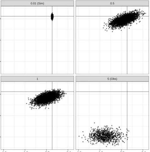
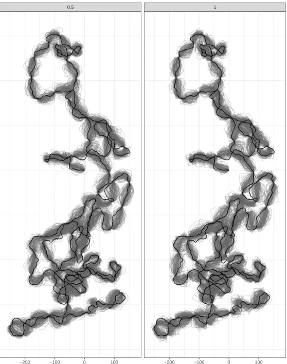
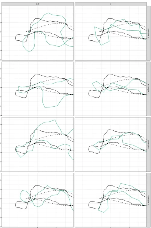
In Chap. 3 we introduce the proposed model for continuous-time single state movement based on step lengths and turning angles. This model formulates movement based on the popular step-and-turn varieties, using bearing and speed processes as analogues for these metrics in continuous time. This chapter begins by creating movement patterns comparable to the discrete-time Morales et al. (2004), but in Sect. 3.4 we propose an alternate model that includes correlation to the speed process in addition to the bearing. We outline a method for Bayesian inference in the form of an augmentation approach inspired by the techniques discussed in Chap. 2. These methods are then demonstrated with applications using simulated datasets. In these examples, inference is also carried out at the observation time-scale, highlighting the bias in estimation encountered in a ‘discrete-time style’ analysis. Chaps. 4 and 5 extend the single state movement model to incorporate the aims listed above; multistate behavioural switching and the presence of observation error, respectively. We introduce behavioural switching through a continuous-time Markov chain (CTMC) based on current approaches in Chap. 2. Examples demonstrate the ability of the inference process using simulated data, and well-known data of elk movements compares these methods with popular discrete-time HMMs. In the observation error case, we first introduce an independent model for error and then extend this in Sect. 5.6 to incorporate correlation. We apply single state movement with error to data from reindeer, and two-state movement with error to observations of a lesser black-backed gull. A simulation example explores the ability to estimate both movement and error parameters simultaneously.

In Chap. 6 we discuss the methods presented in Chaps. 3–5 and how they fit within the current state of continuous-time animal movement in Chap. 2. We provide suggestions for future work.

(34)

(35)

Chapter 2 Review of continuous-time modelling

Continuous-time movement models can be seen as the ‘gold standard’ of movement mod-elling, avoiding the challenges of discrete time through being scale-invariant and respecting the continuous nature of an animal’s movement (see the discussion on the formulation of time in Sect. 1.3). Although a number of models formulated in continuous time exist, their uptake has been somewhat lagging in comparison to the discrete-time step-and-turn models of Sect. 1.2. Such limited application has mainly been rationalised by the often inaccessible parameter interpretation and computational demand of continuous-time meth-ods. The following chapter outlines the existing continuous-time methods for modelling animal movement data that this thesis aims to build upon to provide intuitive and understand-able methods. The following is an extension to the author’s edited contribution within the published review Patterson et al. (2017).

2.1 Modelling movement with diffusion processes

Animal movement models formulated in continuous time are usually based on diffusion processes—continuous-time Markov processes that are the solution to some set of stochastic differential equations (SDE). Such processes suit animal movement because their sample paths are (almost surely) continuous and can contain randomness. Linear, Gaussian diffusion processes are tractable, and can be ‘combined’ to produce a flexible range of possible trajec-tories. This section explores the current approaches to modelling movement in continuous time by focusing on the diffusion processes that form the ‘building blocks’ underpinning such models.

(36)

16 Review of continuous-time modelling

2.1.1 Brownian motion

The simplest diffusion process is Brownian motion (BM, or Wiener process), a Gaussian process with continuous paths and independent increments such that

W(t)∼N(0, t), (2.1) withW(0) =0 and Cov(W(t),W(s)) =sfors≤t. BM can be characterised as the continuous-time limit of a simple random walk (Iacus, 2008) and is an important component for more sophisticated diffusion processes, such as those in the following sections. Extending tod

dimensions, BM is generalised as

W

WW(t)∼Nd(000, tΣ),

whereΣis thed-dimensional covariance matrix that scales standard BM in each dimension.

Given a sequence of observations{xxx(tj)}from a process following BM, the likelihood of

such involves the product over each multivariate normal density describing the independent increments of the process;

p {xxx(t_j)} |Σ=

_∏

j

(2π)−d/2|∆tjΣ|−1/2exp(−(∆x′j(∆tjΣ)−1∆xj)/2),

where∆xj=xxx(tj+1)−xxx(tj)and∆tj=tj+1−tj.

Thed-dimensional process derived from BM that is constrained to start atxxxat timesand end atyyyat timeuis referred to as the Brownian bridge (BB, Iacus (2008)), defined fors≤t≤u

in terms of BM as W W Wu_s,,xxxyyy(t) =xxx+WWW(t−s)− t−s u−s WWW(u−s)−yyy+xxx ,

whereWWW is Brownian motion so that

W W W(t−s) W WW(u−s) ! ∼N2d   000 000 ! , t−s t−s t−s u−s ! Σ  .

HenceWWWu_s,,xxxyyy(t)is given by the multivariate normal distribution

W WWu_s_,,_xxxyyy(t)∼N_d xxx+t−s u−s(yyy−xxx), (u−t)(t−s) u−s Σ . (2.2)

(37)

2.1 Modelling movement with diffusion processes 17

2.1.1.1 Brownian motion as a model for position

As a model for animal movement, BM is simplistic, representing movement that is unbiased, undirected and has no interaction with the environment. For this reason, it is only of use either as a component within a switching model (implicitly in Blackwell (1997, 2003), see Sect. 2.3) or as a purely local model such as Horne et al. (2007). Movement between consecutive, known locations is estimated by the use of Brownian bridges, scaled by a volatility parameter. Inference in Horne et al. (2007) involves learning about the variance parameter of BM, with observations having the likelihood given by Eq. 2.2. Given multiple observations, the product is taken over each disjoint BB formed between pairs of successive locations. Because the distribution of an animal’s location at any time is normally distributed with the estimated variance, quantile regions can be calculated with ease. This kind of interpolation is informative about utilisation distributions—the marginal distribution of an animal’s location— and hence habitat use.

Spatial observation error is accounted for in the BB model of Horne et al. (2007) by assuming independent, identically distributed (iid) normal perturbations with known variance. In this case inference uses a ‘leave one out’ approach, removing alternate observations and essentially using only part of the information provided by observations for inference. An extension enabling estimation of the observation error parameter is not provided and so sensitivity analysis based on the chosen value is important.

2.1.2 Ornstein-Uhlenbeck process

The Ornstein-Uhlenbeck (OU), or Vasicek, process (Uhlenbeck and Ornstein, 1930) is the solution to the SDE

dU(t) =β µ−U(t)dt+σdW(t),

whereW(t)is BM. This stationary, Gaussian process is mean-reverting (Dunn and Gipson, 1977), and so has a tendency to drift towards its long-term mean. The process is given in terms of BM as U(t) =µ+σe −βt p 2β We2βt,

distributed (based on Eq. 2.1 and Iacus (2008))

U(t)∼N µ, σ

2

2β

! .

(38)

The process at a future point in time, given the current valueU(0) =u0, is

U(t) =µ+ (u0−µ)e−βt+ σ p 2β W e2βt−1 e−βt,

having the conditional distribution (again, based on Eq. 2.1)

U(t)|U(0) =u0∼N µ+ (u0−µ)e−βt, σ 2 2β 1−e−2βt ! .

Extending toddimensions, the stationary and conditional distributions, respectively, of the OU process are U UU(t)∼Nd(µµµ,Λ), UUU(t)|UUU(0) =uuu0∼Nd µ µ µ+ (uuu0−µµµ)eBt, Λ−eBtΛeB ′ t , (2.3)

where µµµ is ad-dimensional vector, Λis ad×d covariance matrix, and Bis a stabled×

dmatrix—that is,eBt→0 ast→∞(Blackwell, 1997; Dunn and Gipson, 1977). Henceµµµ

describes the centre of the process, with rate of attraction towards the centre controlled byB

and with random variation governed byΛ.

In two dimensions, the distribution of the OU process is unimodal and elliptical. It is worth noting here the special, circular case in which the matrices B,Λ are isotropic, i.e.

symmetric under rotation and reflection so thatB=βI2,Λ=σ

2

2βI2, withβ <0. In this case

the attraction towards the centreµµµ is determined only by the current displacement from the

centre rather than by direction and no significance is placed upon the dimensional system chosen (Blackwell, 1997). Further, this simplified case is equivalent to two independent, one-dimensional OU processes with parametersµi,β,σ2.

2.1.2.1 Ornstein-Uhlenbeck process as a model for position

Dunn and Gipson (1977) gave the first method for modelling animal positions in continuous time, describing two-dimensional positions by an OU process. This kind of process can be informative about the home range of an animal—the spatial range in which it performs its daily activities (see recent discussion/review by Börger et al. (2008)). This is often mathematically defined as the smallest geographical area in which the animal spends a fixed proportion of time and can be estimated by the equilibrium distribution of the OU process,

(39)

2.1 Modelling movement with diffusion processes 19

similar to the Gaussian home ranges estimated in Jennrich and Turner (1969). Inference for the OU parameters in Dunn and Gipson (1977) uses maximum likelihood, based on the animal beginning movement under its equilibrium distribution and successive observations arising from the conditional distribution.

The OU process addresses the problem of autocorrelation of position, meaning high frequency ‘bursts’ of observations can be modelled. The OU process, however, will always result in an estimate of home-range being elliptical and unimodal. For some animals and habitats this will not be an appropriate assumption (Blackwell, 1997). As with BM, this limits usefulness as a lone model for movement, but it is an important component in constructing more realistic models (see Sect. 2.3).

2.1.2.2 Ornstein-Uhlenbeck process as a model for velocity

The continuous-time model of Johnson et al. (2008a) takes the popular movement assumption of a CRW by directly modelling the velocity, rather than position, of the animal. The velocity describes the instantaneous rate of change of location, modelled as a bivariate OU process. In practice, Johnson et al. (2008a) use two independent one-dimensional OU processes (the circular case described above) as they argue that a non-zero correlation in the velocity process would lead to unrealistic movement patterns. The persistence assumption, that an animal will likely keep moving in a similar direction over a short period of time, is incorporated as a result of the autocorrelation of the OU process. The location of the animal at any time,t, is found by integrating the velocity process

zzz(t) =zzz₀+ Z t

0

vvv(u)du.

This results in the location process no longer being Markovian—as in the OU position model above—as it depends on the entire velocity process prior to timet. However, the combined process of position and velocity is Markovian.

Observation error in position is incorporated into Johnson et al. (2008a) via a SSM (see Sect. 1.2.2) with Gaussian distributed errors. Unlike Horne et al. (2007), the parameters describing observation error in Johnson et al. (2008a) are not assumed known and are estimated as part of the inference process. In relation to the SSM definition of Sect. 1.2.2, the observation equation,Z_t∗, describes the observed location and the process equation,Z_t, describes the joint process consisting of the true location and the velocity (because this joint process is Markovian). Using the SSM framework, Johnson et al. (2008a) use the

(40)

Kalman filter (introduced in Sect. 1.2.2) to carry out statistical inference. The Gaussian error assumption and the linearity of the OU velocity process are necessary for the Kalman filter to be valid. The algorithm provides optimal estimates of the processZt (the unobserved true

locations of the animal as well as the velocity at each observation time) and uses maximum likelihood to estimate the OU process parameters and the observation error variance. Further, the Kalman filter can also estimate the location and velocity at missing observation times. As mentioned above, estimating the home range of an animal is a common metric in move-ment analyses. The true locations estimated in the Johnson et al. (2008a) method can be used to calculate the animal’s home range, with a popular method for this being kernel density estimation. However, a key assumption of such a method is that observations are independent, yet the locations of an animal are highly correlated. Further, features such as irregularity in time that cause ‘bunches’ of similarly timed observations to exist bias density estimates. An extension to Johnson et al. (2008a) is given in Johnson et al. (2011) that allows estimation of movement summaries, such as home range, in a rigorous way. A Bayesian data augmentation approach is taken in which samples of the unobserved location process are drawn and used to gain a Monte Carlo estimate of the summary statistic of interest, allowing uncertainty to be properly quantified.

Applying the Kalman filter for statistical inference involves assuming that observation errors are normally distributed. This assumption is often questioned for some tracking technologies due to the presence of large outliers (e.g. marine animals observed inland) and is thought to be modelled more closely by at-distribution that can allow for large errors through heavier tails (Jonsen et al., 2005). An extension to Johnson et al. (2008a) is presented in Albertsen et al. (2015) that usest-distributed errors rather than Gaussian. In order to carry out statistical inference (because the Kalman filter can no longer be applied), the Laplace approximation is used to evaluate the integral of interest, in this case integrating over the unobserved true locations. Using simulations, Albertsen et al. (2015) show that this method improves upon true location estimation through the heavy-tailed error distribution.

2.2 Modelling movement with general SDEs

The diffusion processes of the previous section arise as solutions to particular cases of the general SDE

(41)

2.3 Modelling switching behaviour 21

A more flexible modelling approach can be achieved by describing movement by an SDE but without the restriction of needing to find a solution to such. This flexibility is generally at the expense of computational, and hence statistical, tractability. A number of approaches consider the case where the SDE derives from basingb(·)in Eq. 2.4 on the gradient of a harmonic function (Brillinger et al., 2002; Brillinger and Stewart, 1998; Preisler et al., 2004, 2013). Such a function represents the animal’s attraction/repulsion to a particular point, line or region in a general way. Brillinger and Stewart (1998) and Brillinger et al. (2002) use specific models that incorporate spherical geometry to allow for a natural representation of long-range migration along great circle routes. Preisler et al. (2004, 2013) present more general models, which also include the special, tractable cases of Sect. 2.1.

Some element of approximation is required to fit models of this general type. Typically, this involves a normal approximation to the movement at each observed time-step. An approximate likelihood can then be derived and maximised; the quality of the approximation obviously depends on the frequency of the data compared with the true rates at which

b(·),σ(·)vary.

More sophisticated approaches to inference from SDEs are available, but are rarely used in a movement context because of the extra computational cost, particularly in the presence of measurement error. A recent advancement in this area is that of Scharf et al. (2017), where a range of movement types can be proposed by a general SDE. Although inference cannot be carried out directly, an augmentation technique is used via multiple imputation, in which the unobserved movement path is simulated multiple times from an approximate imputation distribution (such as Buderman et al. (2016) or Johnson et al. (2008a)). A Markov chain Monte Carlo (MCMC) sampler can be used to make inference about the movement parameters based on the imputed paths. This approach provides flexible modelling options, but relies heavily on the assumptions of the approximate imputation distribution.

2.3 Modelling switching behaviour

Animal movement cannot be homogeneous over an extended period of time, yet incorporating heterogeneity into a continuous-time framework has not been widespread. In the velocity model of Johnson et al. (2008a) behavioural switching is highly restricted, included only as a covariate that acts on movement by setting the velocity to zero to create a stationary state at known times (these times are based on additional tag information). Similarly limited scenarios include diffusive movement (e.g. BM or correlated velocity) where parameters are

(42)

dependent upon the discrete location of the animal (Ovaskainen, 2004; Ovaskainen et al., 2008), simplifying to a discrete-time behavioural process (Hanks et al., 2011; Kranstauber et al., 2014; McClintock et al., 2014) or movement process (Breed et al., 2012; Jonsen et al., 2005).

The following explores a number of different approaches to modelling that aim to incorporate heterogeneity in the movement process with time and (in a limited number of methods) environment. It is important to note that in all the following cases, while it is convenient to refer to the ‘behaviour process’, the behavioural state potentially has limitations; that is, the state may reflect a statistical description of movement rather than necessarily being ‘behaviour’ in a true biological sense.

2.3.1 Movement measures

A number of studies have used movement measures to describe and explore types of move-ment modes. A popular measure is the level of autocorrelation between the step lengths calculated from observations (Boyce et al., 2010; Gurarie and Ovaskainen, 2011). The sample autocorrelation function (ACF) is calculated for each time laghas

ACF(h) =M(h) −1 ∑M_i₌(₁h)(xi−x¯)(xi+h−x¯) M−1 ∑Mi=1(xi−x¯)2 ,

whereMis the total number of observations,M(h)is the number of pairs of observations at time laghand ¯xis the sample mean. By estimating the ACF over the range of time lags between the sampling frequency and period, this gives an indication of the properties of the time series, such as its order of autoregression. Other measures exist that attempt to classify movement over time, but are often overly simplistic. These include calculating a sinuosity/‘straightness’ index by taking the straight-line distances travelled between observed locations (Bovet and Benhamou, 1988; Postlethwaite et al., 2013), the first-passage/residence time calculated as the time required to cross a circle of given radius (Barraquand and Benhamou, 2008; Fauchald and Tveraa, 2003; Lavielle, 2005), and fractal analysis methods that estimate the degree with which an area has been covered by the animal (Tremblay et al., 2007). In all cases, these measures can only be used as exploratory tools and are sensitive to the observation sampling frequency because they often rely on derived quantities such as step lengths.

The ACF calculation above requires estimation of the mean and variance of the full time series, yet the usual estimators for these quantities are unreliable when data is highly correlated. In

(43)

2.3 Modelling switching behaviour 23

contrast, the semivariance function (SVF) contains equivalent information to the ACF, but avoids estimation of the mean and variance. The SVF measures the variation in a series over all possible time lags spanning between the sampling frequency and the overall period, given as SVF(h) = 1 2M(h) −1 M(h)

∑

i=1 (x_i₊_h−x_i)2,

for lagh. Further, the statistical properties of the SVF are more tractable than the ACF, being

χ2-distributed for a given lag when the underlying process is Gaussian. Based on this, a

robust statistical modelling approach is given in Fleming et al. (2014a,b) using measures of correlation to identify trends in movement at different time scales.

Fleming et al. (2014a) give the empirical form of the SVF in terms of a set of movement parameters for a number of popular models, including BM and the OU process, along with mixtures of models, such as the OU process interspersed with random bouts of foraging activity. Hence, a flexible range of movement models are considered. The non-stationarity of movement data due to cycles (such as seasonality) results in the SVF depending not only on the lag but also the absolute times of the observations. To handle this, Fleming et al. (2014a) adjust the process by taking a time-average that treats the non-stationarity as a nuisance factor and leaves only the lag dependence. Given observations, weighted least-squares regression is used to estimate the parameters in the SVF for each movement model and information criterion is used for model selection. This technique enables identifying and making inference on both the different movement behaviours associated with an animal’s trajectory and the temporal scales over which these behaviours occur. The inference approach of Fleming et al. (2014a) is improved upon in Fleming et al. (2017) by using the Kalman filter (see Sect. 1.2.2) to speed up the model fitting process.

Fleming et al. (2014a) is limited by an inability to associate behaviours directly with environ-mental information or identify the specific behavioural state employed at any one point in time. Although this problem is still unsolved, a step towards this end is given in Fleming et al. (2016), presenting methods for inferring the full movement (but not behavioural) trajectory of the animal. This involves estimating the density of space use between observed locations. As described in Sect. 2.1.1.1, the BB is often used as a model for between-observation locations, but is overly simplistic. In Fleming et al. (2016), the more sophisticated movement models of Fleming et al. (2014a) are used to estimate the space use density. This approach relies on each model being Gaussian, enabling estimation of the location at unobserved times, conditional upon the observed locations and chosen model.

(44)

Another step towards identifying the behavioural changes in movement models of this form is Gurarie et al. (2017), concerned in particular with identifying movement behaviours with much longer time frames than home ranging and foraging (such as migration). This method attempts to improve upon the simple methods commonly used for this type of identification, such as spatial clustering. The location process is the sum of a mean process, m(t), and an autocorrelated fluctuation process,r(t). A ‘range shift’ is defined as altering the mean process, with a simple shift example being

m(t) =        m₁ ift<t₁, m1+(m2−_tm₂₋1)(_t₁t−t1) ift1≤t ≤t2, m₂ ift>t₂,

however more sophisticated models with features such as ‘stopovers’ could be used. In the case above, the animal has two centres of movement,m1andm2, with a linear process

controlling the shift between these centres. The autocorrelated fluctuation process then defines the type of movement around the centre, with standard forms being given for all the movement models discussed in Fleming et al. (2014a). Inference in Gurarie et al. (2017) is by likelihood methods similar to Fleming et al. (2014a).

2.3.2 Change point analysis

Gurarie et al. (2009) describe a model that is able to identify heterogeneity and characterise movement within each ‘behaviour’. Their approach is then applied and compared with those including the first passage time of Fauchald and Tveraa (2003) and the multistate random walks of Morales et al. (2004). The underlying movement is parametrised by orthogonal quantities, coined as ‘persistent’ and ‘turning’ velocities, assumed to follow stationary, autoregressive Gaussian processes; each described by a mean, variance and autocorrelation parameter. The persistent and turning velocities are derived from speeds and turning angles, calculated as averages between observations, hence the reliability of this method will vary for irregular datasets.

Given a series of movement observations and the time of a single behavioural switch, the likelihood for the process parameters is simply the product of the two Gaussian functions. A single behavioural change-point is estimated by maximising this likelihood over all possible switching times. In turn, the parameters for each behavioural state are estimated by maximum likelihood using the observations from the respective behavioural state. The method is extended to any number of behavioural states and change-points by passing a

Bayesian inference for continuous-time step-and-turn movement models