Efficient Algorithms for Finding Optimal
Binary Features in Numeric and Nominal
Labeled Data
Michael Mampaey
1, Siegfried Nijssen
2,3, Ad Feelders
4, Rob Konijn
2,5, and Arno Knobbe
2 1University of Bonn, Germany2Leiden University, The Netherlands 3KU Leuven, Belgium
4Utrecht University, The Netherlands 5VU University Amsterdam, The Netherlands
Abstract. An important subproblem in supervised tasks such as decision tree induction and sub-group discovery is finding an interesting binary feature (such as a node split or a subsub-group re-finement) based on a numeric or nominal attribute, with respect to some discrete or continuous target variable. Often one is faced with a trade-off between the expressiveness of such features on the one hand, and the ability to efficiently traverse the feature search space on the other hand. In this article, we present efficient algorithms to mine binary features that optimize a given convex quality measure. For numeric attributes we propose an algorithm that finds an optimal interval, whereas for nominal attributes we give an algorithm that finds an optimal value set. By restricting the search to features that lie on a convex hull in a coverage space, we can significantly reduce computation time. We present some general theoretical results on the cardinality of convex hulls in coverage spaces of arbitrary dimensions, and perform a complexity analysis of our algorithms. In the important case of a binary target, we show that these algorithms have linear runtime in the number of examples. We further provide algorithms for additive quality measures, which have linear runtime regardless of the target type. Additive measures are particularly relevant to feature discovery in subgroup discovery. Our algorithms are shown to perform well through experimen-tation, and furthermore provide additional expressive power leading to higher-quality results. Keywords: Binary features, decision trees, subgroup discovery, numeric data, nominal data, la-beled data, convex functions, convex hulls, coverage space, ROC analysis
Received Mar 09, 2013 Revised Aug 16, 2013 Accepted Sep 07, 2013
1. Introduction
Many tasks in data mining are supervised in nature: one wishes to predict or characterize a given target attribute. Important methods that can be used to solve such tasks are those that findsymbolicmodels or descriptions of data. Well-known examples of symbolic predictive models are decision trees, regression trees, and rule-based models. Subgroup discovery (SD) is an important example of a descriptive data mining task [Herrera et al., 2010, Kl¨osgen, 2002, Wrobel, 1997]. A characterizing feature of these symbolic models and patterns is that they are built fromconditionson attributes: in decision trees, internal nodes consist of attribute-value conditions; in rule-based models and subgroup discovery, rules consist of conjunctions of conditions on attributes.
As an example, consider the problem of subgroup discovery in the context of fraud detection in a medical insurance dataset. The aim is to find subsets of the data where the distribution of a (binary) target variable is substantially different from its distribution in the whole data, assessed by a quality measure [Kl¨osgen, 2002, Wrobel, 1997]. The data contains records about all claims (treatments) that were made over a certain period. We are investigating a specific medical practitioner, say a dentist, and define a target concept to reflect this: positive cases are claimed by the dentist under investigation, negative cases are claimed by one of the other dentists. We look for conditions on the attributes, such that claims satisfying the conditions (members of thesubgroup) are from the dentist in question significantly more than when taking a random sample. As such, the attribute conditions featuring in the subgroup description provide information as to the value of the target. In this dataset, subgroup descriptions could consist of (conjunctions of) conditions such as
Age≥67 and Age<15∧Treatment =E13: root canal treatment. Similarly, when learning decision trees on this data, we could look for attributes of the claim (treatment codes, costs, patient details, . . . ) on which we can perform tests that ‘predict’ the dentist of interest.
Clearly, when finding such symbolic models or subgroup descriptions, an important choice to make is which conditions to consider. In most symbolic models, these are equalities for nominal attributes (such asTreatment =E13: root canal treatment) and inequalities for numeric attributes (such asAge≥67). Important reasons for choosing these conditions are that they are easy to interpret, and that they can be found reasonably efficiently.
Straightforward algorithms for finding good combinations of conditions can be computationally demanding. For instance, discovering a combination of constraints on a patient’s age, such as18≤Age ≤67, would involve a quadratic number of calculations (with respect to the number of threshold values considered) to find the optimum.
To avoid this complexity, most well-known methods apply a greedy search strategy that finds thresholds while searching for models: a number of potential cut-points of a given numeric attribute is computed on the fly, by considering the subset of data currently under investigation. In decision trees, this subset concerns the examples that fall in the current branch to be split, whereas in SD, it concerns the examples in the current candidate subgroup that needs refining. Only the most promising splits are considered further. Whereas this makes the search feasible, it also limits the models or SD descriptions that can be found.
In this article we propose an improvement of this state of the art of symbolic modeling and subgroup discovery, based on the observation that a larger space of conditions allows for finding models and patterns of higher quality. The improvement consists of efficient algorithms for finding two fundamental types of conditions: intervals for continuous
attributes, and value sets for nominal attributes. We prove that in the binary case, under reasonable assumptions, the best scoring such conditions can be found without increasing the computational complexity of symbolic modeling or subgroup discovery systems.
Interval conditionsare of the formAge ∈]18,35]. They allow us to focus directly
on ranges of values of interest. Such conditions are hard to find by traditional greedy algorithms, as they would need to find the conditionsAge>18andAge ≤35in two stages. A straightforward algorithm would involveO(N+t2)calculations, whereNis
the number of examples in the current node or subgroup, andtis the number of possible thresholds. Instead, we propose a new efficient algorithm that can directly mine the best scoring specialization of a rule or model over all possible intervals. We show that in the important binary case, an optimum can be found inO(N+t)time, for any convex quality measure; hence, finding an interval is not more expensive than finding an inequality such asAge>18and is feasible even on large datasets.
Set-valued conditionsare conditions of the formTreatment ∈ {M55: dental cleaning,
V21: polishing a filling,V11: one-sided filling}. It is likely that considering an
individ-ual treatment does not result in a subgroup indicative of fraud by a specific dentist, while an unusual combination does (certain combinations of treatments are actually not permitted). As such, if we only consider single values of nominal attributes, we miss out on some potentially useful subgroups. To some extent this can be alleviated by imposing a hierarchy on the attribute values, but such a hierarchy would have to be specified by the user and still considerably restricts the number of possible groupings. We can avoid such problems by directly searching for an optimal subset of attribute values. We present an algorithm that finds an optimal set in polynomial time, and prove that in the important binary case its runtime isO(N+d), wheredis the size of the attribute domain. We further prove that with a straightforward optimization, the algorithm presented by Breiman et al. [1984] for binary targets can be implemented to run in linear time with respect to the number of examples, rather than linearithmic time. To the best of our knowledge, this is a novel result.
From a theoretical perspective, the above algorithms can easily be added to greedy symbolic modeling systems and subgroup discovery systems. In the very common binary case, this can even be done without affecting their asymptotic runtime complexity. How-ever, as the algorithms are conceptually more involved, it may be harder to implement them efficiently. We address this issue by showing that simpler algorithms can be used for additive quality measures such as Weighted Relative Accuracy (WRAcc), which are particularly relevant in subgroup discovery.
Note that every condition can be seen as a new binary feature: instead of including the testAge ≥67in a rule, we could also have included an additional column in our data with boolean values representing the truth ofAge≥67. A rule or tree could then be represented by conditions on these boolean attributes; hence, finding conditions also amounts to identifying interesting boolean features for an originally non-boolean dataset.
In the remainder of this article, we mostly use subgroup discovery as an example for the application of our algorithms; however, it should be stressed that the algorithms can also be used in other tasks, such as decision tree learning, regression tree learning, and the induction of rule-based predictive models, which are algorithmically closely related. This is despite the fact that the goals of subgroup discovery and, e.g., classification are distinct: a classifier is a global predictive model, whereas a subgroup is a local descriptive pattern. A good subgroup is therefore not necessarily also a good classification rule or vice versa. Many subgroup discovery quality measures are asymmetric, considering only the subgroup itself, whereas a node split in a decision tree takes into account the impurity of all its child nodes. Moreover, the impurity of a split in a decision tree is measured against the class distribution in the parent node, whereas a subgroup (refinement)’s quality is
compared against the global target distribution. That being said, from an algorithmic perspective the techniques presented here are readily applicable in all these areas.
This article is structured as follows. First, we discuss related work in Section 2. In Section 3, the necessary preliminaries and notation are introduced. Section 4 discusses convex hulls and coverage spaces, and some general theoretical results. Then, in Sec-tions 5 and 6 we present two algorithms to efficiently find optimal features in the form of intervals and value sets, for numeric and nominal attributes, respectively. In Section 7 we experimentally evaluate these algorithms on synthetic and benchmark data, as well as on a real-world health insurance dataset. Finally, we end with conclusions in Section 8.
2. Related Work
The discovery of conditions is required in several important supervised mining tasks, including predictive modeling tasks and subgroup discovery or pattern mining tasks.
Subgroup discovery and pattern mining In subgroup discovery and supervised pattern
mining, the goal is to find symbolic descriptions for subgroups of the data in which the distribution of a target attribute is significantly different from the distribution for the whole dataset; hence, a fixed target attribute is assumed, in contrast to what is common in association rule discovery [Agrawal et al., 1993, H¨am¨al¨ainen, 2012].
Usually, the symbolic descriptions consist of conjunctions of conditions. The simplest case is the one in which the data is binary; conditions in this case only need to test the truth value of the features. Subgroup discovery, and more generally pattern mining, is dominated by algorithms that are restricted to such discrete data.
The algorithms that find subgroup descriptions or patterns can be categorized into two classes: those that perform an exhaustive search under constraints, and those that are greedy. In particular exhaustive search algorithms that operate directly on numerical data face large computational challenges if no strong restrictions are applied.
Grosskreutz and R¨uping [2009] propose an exhaustive algorithm for mining top-k
subgroups in numeric data. Their approach returns thekglobally best subgroups using interval descriptions, for a family of quality measures that includes WRAcc. The method is defined purely for numeric attributes, rather than heterogeneous data. Search space pruning is achieved by using a data structure that maintains optimistic estimates for attributes; only the size of this data structure is already quadratic in the number of split points in the worst case.
Fukuda et al. [1999] present two algorithms for mining optimal association rules. The search is made feasible by limiting the search to rules of the formA∈[l, r]⇒C, for a fixed numeric attributeAand (binary) consequentC, in the well-known support-confidence framework, optimizing for one measure whilst using a threshold for the other. The threshold is necessary in order to avoid discovering trivial rules. These algorithms have linear runtime, but are specific to the support and confidence quality measures, and work in a support-positive support space rather than in ROC space.
To avoid a large computational complexity, and to be able to find conjunctions of conditions, most subgroup discovery systems that operate on numerical data either perform pre-processing of numeric data or avoid exhaustive search altogether. In both cases, there is the risk of losing information [Atzm¨uller and Puppe, 2006, Kavˇsek et al., 2003]; however, the advantage of systems that do not rely on exhaustive search is that it more feasible to perform discretization during the search.
A good example of a system that performs on-the-fly discretization is Cortana [Meeng and Knobbe, 2011]. While searching for subgroup descriptions, it searches for inequality
conditions for numerical attributes, and allows for on-the-fly binning; its search is greedy as the search only continues for the best conditions found.
The algorithms studied in this work are specifically aimed for systems of this kind, which can be characterized by these two properties:
– they use heuristics to search through a space of conjunctions;
– during the search they repeatedly perform discretization for subsets of the same data. The latter property is important, since it means that it may pay off to perform calculations (such as sorting the data) before the search is started. The first property is important, since it means that these systems may not be able to find good conjunctions of conditions through search. Only by a sufficiently broad set of conditions can the discovery of certain subgroups be ensured.
To find good conditions in a greedy search, subgroup discovery algorithms often use similar algorithms as decision tree learning algorithms, as discussed next.
Decision Trees In decision trees, an important challenge is how to find the conditions
that are put into the internal nodes of the trees. Most algorithms operate in a top-down greedy fashion, and hence also perform a repeated search for conditions in subsets of the data [Breiman et al., 1984, Rzepakowski and Jaroszewicz, 2012].
A numeric attribute at a given node in a decision tree is typically split intokchild nodes, usingk−1threshold values (oftenk= 2). How to find a good split point has been the topic of several past studies.
Fayyad and Irani [1993] proved that for a convex impurity measure, an optimal split point must always be a boundary point, that is, a point for which the two adjacent values on either side of the split point have distinct labels (assuming no duplicate values occur). This was generalized by Elomaa and Rousu [2004], who showed that a threshold in an optimalk-way split never separates two adjacent base intervals with an equal class distribution. The number of potential split points can thus be reduced considerably, in linear time with respect to the number of data points. Fork= 2, finding the optimal split clearly takes linear time; fork≥3, the optimalk-way split can be found in quadratic time with respect to the number of split points, using dynamic programming.
The algorithms that we will propose in this article are related to these earlier al-gorithms; however, in contrast to these earlier algorithms, we use two thresholds (the interval endpoints) to define a binary split, i.e., we separate data points within the interval from those outside of it.
As conditions for nominal attributes, decision trees can either perform ad-way split on all possible values (wheredis the domain size of the attribute), or can search for the optimal subset of values (and its complement), to split the node into two child nodes. Such a node splitting algorithm is used by CART [Breiman et al., 1984], which works with a binary target.
A contribution of this work is that we will show that a straightforward optimization lowers the complexity of this algorithm fromO(N+dlogd)toO(N+d).
Chou [1991] presented an approximate technique to find a good split of a nominal attribute. This algorithm uses ak-means-like approach, which is justified by the obser-vation that a globally optimum solution must satisfy a nearest neighbor criterion. For binary splits specifically (as considered in this article), the complexity isO(dc)per iteration, wheredis the size of the domain andcis the number of classes of the target. The number of iterations required until convergence, however, is not known beforehand, and moreover, the result is only an approximation of the optimal solution.
3. Preliminaries and Notation
We assume that we are given a dataset D containing examples~x ∈ D of the form ~
x= (a1, . . . , ak, c), wherekis a positive integer. Eachaiis the value of a corresponding attributeAi, and we write~a= (a1, . . . , ak). We callctheclass labelortarget valueof~x.
Each attribute valueaiis taken from a domaindom(Ai). We consider binary, nominal,
and numeric attributes, that is, attributes for which,dom(A) ={0,1},|dom(A)| ∈N0,
anddom(A) = R, respectively. The target is also allowed to be binary, nominal, or numeric; we focus mostly on the common case of binary targets. The size of the dataset is denoted byN =|D|. If the target is nominal, the subset of the data for which the class is equal toiis written asDi ={~x∈D |c=i}, and its size asNi =|Di|. For
binary targets, these are written asD+andD−to denote the positive and negative part of the data, respectively. If the target is continuous, we consider the meanµ0and standard
deviationσ0of the target.
Definition 1. Afeatureon an attributeAis a binary functionf :dom(A)→ {0,1}.
We consider features that are described as one of four types of basic conditions: 1. equalities:A=a, wherea∈dom(A),
2. inequalities:A≤a, wherea∈dom(A), 3. value sets:A∈V, whereV ⊆dom(A), and 4. intervals:A∈]l, r], wherel < r∈dom(A).
Conditions 1 and 3 are applicable to nominal (including binary) attributes, whereas conditions 2 and 4 are applicable to numeric (and ordinal) attributes. Note that 1 and 2 are in fact special cases of 3 and 4, respectively.
Conditions can be used in patterns, subgroup descriptions and predictive models such as decision trees.
Definition 2. Apatternis a binary functionp:Qk
i=1dom(Ai)→ {0,1}. We assume
that a pattern is described by a conjunction of features, that is, a conjunction of conditions on the attributes. A patternpis said tocover a data point~x = (~a, c)if and only if p(~a) = 1. Asubgroupcorresponding to a patternpis the bag of data pointsGp ⊆D
that are covered byp:
Gp={~x∈D|p(~a) = 1} .
If no confusion can arise, we omit the subscriptp. We writen = |G|for the size of G. If the target is nominal,nidenotes the number of examples of classiinG(hence
P
ini=n), whereas if the target is continuous, writeµandσfor the mean and standard
deviation of the target withinG. The complement of a subgroup is written asG=D\G, and its size asn=G.
Similarly, we can use conditions to construct binary decision trees.
Definition 3. A binarydecision treeis a binary tree in which every internal node
corre-sponds to one of the basic conditions, and every leaf is labeled with a class label. Despite the differences between trees and subgroup descriptions, the search for both tasks proceeds in a similar way. The search starts from an empty pattern or tree, and iteratively conditions are added to the pattern or the tree.
The space of candidate patterns in subgroup discovery can be organized in a lattice; by iteratively adding conditions, subgroup discovery algorithms traverse this lattice in a top-down, general-to-specific fashion. Which conditions are added is determined by a
refinement operatorρ:P →2P, a syntactic operation which determines how simple patterns can be extended into more complex ones by atomic additions.
One can distinguish between exhaustive search algorithms, which explore all possible refinements, and greedy algorithms, which only explore the best scoring refinement according to a heuristic.
In decision tree learning, the standard approach is a top-down approach, in which first the root of the tree is searched for using a heuristic; the examples of the data are sorted in the left-hand or the right-hand subtree, based on the condition put in the root of the tree. The search for further refinements proceeds recursively for the left-hand child and the right-hand child of the root.
In both cases, in order to find a good candidate feature, aquality measureis used. For a pattern pin the pattern languageP, this is a function that measures how interesting the induced subgroupGpis.
Definition 4. Given a datasetD, aquality measure for patternsis a functionϕD :P →
Rthat assigns a numeric value to a patternp.
For convenience, we also writeϕDas a function of theni, the number of examples in
classiinGp, that is,ϕD(p) = ϕD(n1, . . . , nc)for a nominal target; or asϕD(p) =
ϕD(n, µ, σ)for a numeric target. We again omit the subscript, whenever the datasetD
is clear from the context.
In the case of decision trees, a quality measure is usually evaluated on a single condition only.
Below, we give the definitions of some commonly used quality measures. For more measures, we refer to F¨urnkranz and Flach [2005].
Definition 5. We are given a datasetD of sizeN, with a binary target definingN+and
N−as above, and a patternpwith countsn+andn−.
TheWeighted Relative Accuracyofpis defined as
WRAccD(n+, n−) = n N n + n − N+ N .
TheBinomial test[Kl¨osgen, 2002] ofpis defined as
BinD(n+, n−) = r n N n + n − N+ N .
Weighted Relative Accuracy is one of the most used quality measures in subgroup dis-covery [Kl¨osgen, 2002, Wrobel, 1997]. It strikes a balance between the target divergence of the subgroup and its size. WRAcc is also known under different names in other contexts in data mining, for instance, leverage in association rule mining, see Novak et al. [2009]. WRAcc is an additive function, for which we provide specialized algorithms in Sections 5 and 6. The Binomial test is similar in form to WRAcc, but is weighted by the square root of the relative support of the subgroup. It can be shown to be order equivalent to the standardizedz-score.
As an example of general dimensionality, we consider theInformation Gainquality measure, which is common in decision tree induction.
Definition 6. TheInformation Gainmeasure is defined as
IGD(n1. . . , nc) =h N1 N , . . . , Nc N − n Nh n1 n, . . . , nc n − n Nh n1 n, . . . , nc n
Finally, we consider the following quality measures for numeric target variables.
Definition 7. Letµ0andσ0be the global target mean and standard deviation.
Thestandardizedz-scoreof a patternpis defined as
z(n, µ) = √
n σ0
(µ−µ0).
Thet-statisticof a patternpis defined as
t(n, µ, σ) = √
n
σ (µ−µ0).
As we shall see below, a crucial property for quality measures isconvexity.
Definition 8. A function f : Rk → R is called convex if for anya,b ∈ Rk and
λ∈[0,1]it holds that
f(λa+ (1−λ)b)≤λf(a) + (1−λ)f(b) . If−f is convex,f is called concave.
We assume that the quality measures we use are convex, which is true for most common quality measures, including WRAcc and Information Gain. This can be seen by verifying that their second derivatives are positive everywhere. Unfortunately, some frequently used measures, such as the Binomial test, the standardizedz-score, or the t-statistics are not. However, this need not always be problematic. For instance, the Binomial test is convex if Bin(n+, n−) ≥ 0, or equivalently, if n+/n ≥ N+/N.
Typically, subgroups for whichBin(n+, n−)<0are not of interest (otherwise we can, for instance, invert the target). Similarly, the standardizedz-score and thet-statistic are convex on the domain wherez(n, µ)≥0andt(n, µ, σ)≥0, that is, whereµ≥µ0. For
our intents and purposes, we can assume that all the quality measures we use are convex. Finally, we also assume that the arguments of a quality measure aremonotonicwith respect to subgroup inclusion. That is, for two subgroupsG⊆G0with corresponding argument valuesxandx0of some (convex) quality measureϕ, it must hold thatx≤x0. If the arguments ofϕare target counts(n1, . . . , nc), it can easily be seen that this holds.
In some cases, however, it may be necessary to rewriteϕ; for instance, we can rewrite the t-statistic as a function of a subgroup’s size, target sum, and target squared sum, which is a set of sufficient statistics for its size, target mean, and target standard deviation.
4. Convex Hulls in Coverage Space
To get some insight into the quality of features, we reason with them incoverage space. First, let us assume that the target attribute is nominal withcclasses, and that we use a quality measureϕ. Typically, the qualityϕof a feature is a function of its countsni
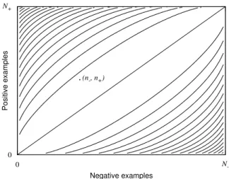
for each classi = 1, . . . , c. Then the associated coverage space is thec-dimensional space[0, N1]× · · · ×[0, Nc]. For a binary labeled datasetD withN+positive andN− negative examples, the corresponding coverage space is the subset[0, N−]×[0, N+]of
the plane—by convention the negative counts are on thex-axis, as shown in Figure 1. In this case coverage space is directly related to ROC space, since the latter is simply a normalized version of the former, rescaled to the unit square [F¨urnkranz and Flach, 2005]. A featurepwith countsnifor each classiis represented by thestamp point
(n1, . . . , nc). An important observation to make is that if the target is nominal, then all
(n-, n+) 0 N -Negative examples 0 N+ Positive examples
Figure 1. Example of a coverage space of sizeN−×N+, a stamp point with coordinates
(n−, n+), and the isometrics of the Information Gain quality measure.
Analogously, if the target is continuous, the coverage space is defined by the domains of the arguments of the quality measureϕ. For example, if we use thet-statistic, whose arguments are the feature size, mean, and variance, the corresponding coverage space is[0, N]×R2. We will see that sometimes it might be convenient to rewrite a quality
measure using other sufficient statistics as its arguments, for instance, writing thet -statistic as a function of feature size, target sum, and target squared sum. In the following, we identify features with their corresponding stamp points in coverage space.
For almost any sensible quality measure, it holds that features that are close to the diagonal connecting(0, . . . ,0)and(N1, . . . , Nc), are considered uninteresting, since
they have approximately the same target distribution as the whole dataset or the parent node; on the other hand, features closer to any of theccorners(0, . . . , Ni, . . . ,0)are
reasonably assumed to have high quality because their target distribution is divergent and pure. For a given quality measure, we can plot its isometrics in coverage space connecting points of equal quality, as shown in Figure 1 for Information Gain in two dimensions.
In our hunt for an optimal feature, let us consider the search space. For instance, for an interval feature on a numeric attribute, the search space consists of all possible intervals whose endpoints are taken from some predefined set, e.g., all distinct values occurring in the data. The stamp points corresponding to the search space are contained
in aconvex hullin coverage space.
Definition 9. Given a set of pointsS inRk, its convex hullCH(S)is defined as the
minimal superset ofSfor which it holds that ifx, y∈CH(S)andλ∈[0,1], then λx+ (1−λ)y∈CH(S).
IfS is finite, it can be seen thatCH(S)forms a convex polytope, and thus can be uniquely identified by its non-degenerate vertices, which we shall denoteH(S). In other words,H(S)consists of all points lying on the ‘edge’ ofS. It follows thatH(S)⊆S, and in practice it often may hold that|H(S)| |S|. In the remainder, we will refer to bothCH(S)andH(S)the convex hull ofS; from the context it should be clear which one is meant.
0 0.1 0.2 0.3 0.4 0.5 0.6 0.7 0.8 0.9 1 0 0.1 0.2 0.3 0.4 0.5 0.6 0.7 0.8 0.9 1
True Positive Rate
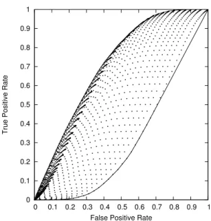
False Positive Rate
Figure 2. The convex hull of a set of points in ROC space. Only the subsets of points that lie on the hull can maximize a convex quality function.
Property 1. LetSbe a set of points in coverage space, and letϕbe a convex quality
measure, then it holds that
arg max
s∈S
ϕ(s) = arg max
s∈H(S)
ϕ(s).
Hence, in order to find an optimal point in the search spaceS, it suffices to only consider the members of the convex hullH(S), rather than the entire set. This fact can be utilized to significantly reduce computation.
An example is given in Figure 2. We selected theAgeattribute from theAdultdataset, which has a binary target attribute [Frank and Asuncion, 2010], and computed the stamp point of every interval featureAge∈]a, b], withaandbtaken from the set of all ages occurring in the data. We now want to find a (not necessarily unique) interval maximizing a given convex quality measureϕ. Since the attribute has 74 distinct values in the data, there are 2 775 possible intervals to consider. However, since only points that lie on the convex hull can maximizeϕ, we only need to consider a small fraction of all intervals. In this example, the convex hull consists of a mere 56 points. If we could directly find those intervals whose stamp points lie on the convex hull, we could save ourselves a lot of computational effort.
Many algorithms that calculate the convex hull of a set of points are to be found in the literature. The Graham scan algorithm is one of several well-known planar convex hull algorithms [Graham, 1972]. Given a set of pointsSin the plane, it computes the convex hullH(S)inO(|S|log|S|)time, or inO(|S|)time if the points are given in some convenient form (e.g., sorted by their polar- orx-coordinates). In three dimensions, O(|S|log|S|)algorithms exist as well, whereas in the general c-dimensional case, the complexity of computingH(S)quickly increases toO|S|bd/2c[Preparata and Shamos, 1985].
We must remark, however, that in our setting we want to directly constructH(S), without having to consider all points inS, all the more since the search space is typically defined implicitly rather than enumerated explicitly. We would therefore like to compute H(S)in time that does not depend too strongly on the search space itself (|S|), but instead preferably depends on the size of the convex hull to be computed,|H(S)|.
To this end, it is useful to investigate just how large a convex hullH(S)can get. The following properties present worst-case upper bounds on the size of the convex hull of sets of points in ac-dimensional discrete coverage space; they are integral to the complexity results presented below. To this end, we start by introducingFarey sets, whose elements will correspond to points (or vectors) in coverage space.
Definition 10. We define a Farey set of orderkand dimensionalitycas the set of all
irreduciblec-tuples of non-negative integers, whose sum is no greater thank, that is, Fkc ={(n1, . . . , nc)∈Nc|gcd(n1, . . . , nc) = 1 andPci=1ni ≤k} .
Note that forc = 2this is equivalent to the standard definition of a Farey set using rational numbers [Conway and Guy, 1996], that is,
Fk2=na
b |gcd(a, b) = 1 and 0≤a≤b≤k o
.
Lemma 1. LetSbe a set of non-negative irreduciblec-tuples, and chooseksuch that
|S|>|Fkc|. DefineR=P n∈S Pc i=1niandQ=Pn∈Fc k Pc i=1ni. ThenR > Q.
Proof. This is a straightforward generalization of Lemma 6.2 in [Calders et al., 2013], a
proof has therefore been omitted.
It immediately follows from Lemma 1 that for a fixedR, the cardinality ofSis at most that of a Farey set for whichQis (approximately) equal toR.1
Lemma 2. Let Fc
k be a Farey set of orderk and dimensionalityc, and define Q =
P
n∈Fc k
Pc
i=1ni. Then|Fkc|is sublinear inQ, specifically,
|Fkc|=OQc/c+ 1 .
Proof. The proof generalizes that of Calders et al. [2013] forc= 2, in which case the
tuples are represented as fractions. Let us denote byZc
kthe number of irreduciblec-tuples
of non-negative integers, each no greater thank. It was shown by Nymann [1972] that Z2
k =k2/ζ(2) +O(klogk), and thatZkc =kc/ζ(c) +O kc−1
forc≥3, whereζis the Riemann-zeta function. In the following, we only consider the case wherec≥3; the casec= 2is similar, whereas the casec= 1is trivially verified. From the inequalities Zc
k/c≤ |F
c
k| ≤Z
c
k, we can derive that
kc ccζ(c)+O k c−1 ≤ |Fkc| ≤ kc ζ(c)+O k c−1 , (1)
and subsequently that there must be somec0∈]0,1]depending only oncsuch that
|Fkc|= c
0 ζ(c)k
c+O kc−1
. (2)
Let us denoteF¯kc =Fkc\Fkc−1, that is,F¯kccontains those tuples whose sum equals exactlyk. It follows that|Fc
k|= Pk l=0 F¯lc
. Now we can write
Q= X n∈Fc k c X i=1 ni= k X l=0 l·F¯lc =k|Fkc| − k−1 X l=0 |Flc| . (3)
Substituting Equation 2, we can calculate Q= c 0 ζ(c) c−1 c k c+1 +O(kc) . (4)
Finally, combining Equations 2 and 4, we have proven that asymptotically
|Fkc|= c 0 ζ(c) ζ(c) c0 c c−1Q c/c+ 1 =c00Qc/c+ 1, (5)
withc00<2sinceζ(c)>1, and therefore
|Fkc|=OQc/c+ 1 . (6)
Property 2. Given a finite set of pointsSin a discrete coverage space of sizeN−×N+,
the number of vertices on the convex hullH(S)is bounded byO N2/3 .
Proof. The proof focusses on the upper left sectionH0of the convex hull; the proof for
the three remaining parts ofH(S)is completely analogous. Let us denote the integer coordinates of the non-degenerate vertices ofH0as(xi, yi), ordered byxi, and define
(ui, vi) = (xi−xi−1, yi−yi−1). Let us writeh=|H0|. Without loss of generality we
assume that(x0, y0) = (0,0)and that(xh, yh) = (N−, N+). It holds that the slopes
vi/uiof the consecutive edges ofH0are positive and strictly monotonically decreasing.
Following Lemma 1, we know that|H0|is maximized if the(ui, vi)’s form a Farey set.
WritingQ=Ph
i=1ui+vi, Lemma 2 tells us thath∈O Q
2/3 . Finally, Q= h X i=1 ui+vi= h X i=1 xi−xi−1+yi−yi−1 (7) =xh+yh (8) =N−+N+=N , (9)
and hence we find that|H(S)| ∈O N2/3 .
What the above property tells us, is that in a two-dimensional coverage space, no matter how many candidate stamps points (corresponding to features) there are, the number of convex hull points that we ultimately need to consider to find an optimum, depends only on the number of examples in the dataset, and moreover, that this number of points issublinearin the number of examples.
Note that this is in fact a worst-case result over all datasets withN examples, for all possible instantiations ofN+andN−. Moreover, in practice we can often expect the convex hull to be quite small. This is exemplified, for instance, by the fact that in expectation, the size of the convex hull of a random uniformly distributed set in the unit square grows only logarithmically in the number of points [R´enyi and Sulanke, 1963].
Corollary 1. Given a set of pointsSin ac-dimensional coverage space×c
i=1[0, Ni],
the size of the convex hullH(S)is bounded byO (N/c)c−4/3 .
Proof. Consider all pointss∈H(S)for which the lastc−2coordinatesn3, . . . , nc
are fixed. This set of points must form a convex polygon, and therefore its size is bounded byO (N1+N2) 2/3 . It follows thatH(S)∈O Qc i=3Ni·(N1+N2) 2/3 = O (N/c)c−4/3 .
Property 3. Given a nominal attributeA, and a discrete target withcclasses, in a dataset
withNexamples, the maximum number of values in the domain ofAwith a distinct class distribution is bounded by
|dom(A)| ∈ONc/c+ 1 .
Proof. Follows from applying Lemma 2 to the class counts of each attribute value.
The crucial requirement in the above properties, is that the coverage space be discrete. If one or several of the dimensions are continuous, Property 2 is no longer valid. If only one dimension is continuous, the complexity of Property 2 increases toO(N), whereNis the size of the discrete dimension. Otherwise, in the worst case all points inScan lie on its convex hullH(S)(for instance, if the points lie on a sphere) and so
|H(S)|can grow arbitrarily large, independent ofN. However, this would require that the coordinates of the points have unbounded precision, which in practice is not the case. If we use, say 32 bit precision reals (or integers), each dimension can in fact be seen as discrete (of size four billion); Property 2 then tells us that the hull size in two dimensions is bounded byO (2·232)2/3
=O 222
, roughly four million, which is still a quite reasonable worst case for large datasets. We show in Section 7 that the algorithms we present can in fact be used for data with a continuous target as well.
The above results tell us something about the number of points on the convex hull that we need to consider in the search for an optimal feature. However, they do not tell us how to consider only these points. To efficiently compute convex hulls in coverage space, we use the concept of aMinkowski sum.
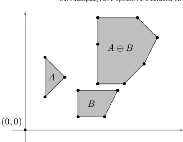
Definition 11. The Minkowski sum of two setsA, B⊆Rkis defined as
A⊕B ={a+b|a∈A, b∈B} .
Figure 3 illustrates the Minkowski sum of two convex polygons. The sum of the bottom left vertices ofAandB, for instance, is the bottom left vertex ofA⊕B.
The following useful properties with regards to Minkowski sums and convex hulls can be observed.
Property 4. For two finite setsAandB, it holds that
H(A∪B)⊆H(A)∪H(B),
CH(A⊕B) =CH(A)⊕CH(B),
|H(A⊕B)| ≤ |H(A)|+|H(B)| .
In the last case, equality holds if and only if all vertices are non-degenerate.
Given two convex polygons in the plane, the convex hull of their Minkowski sum is constructed as follows. Assuming the vertices (and edges) ofAandBare sorted, say clockwise, the corresponding edge lists are merged, sorted by their slopes. Thus, we can compute the convex hull of the Minkowski sum of two convex polygonsAandB, in
(0,0)
A
B
A⊕B
Figure 3. The Minkowski sum of two convex polygons. Each point inA⊕Bis the sum of a point inAand a point inB.
O(|A|+|B|)time. In Figure 3, each edge ofA⊕Bcorresponds to an edge of either AorB. The resulting sum contains one degenerate hull point and henceH(A⊕B)
contains six out of a maximum of seven points. In higher dimensions, based on Property 4, we can see that the convex hull of two convex polytopesAandBcan be constructed by considering all possible pairs of vertices, takingO(|A| |B|)time. This results in a superset of the convex hull, which is consequently computed inO(|A| |B|log|A| |B|)
time in three dimensions, orO(|A| |B|)bd2c
time in general.
5. Interval Features
In this section, we present a general algorithm to find a binary feature of the form A∈]l, r]maximizing a convex quality measureϕ, whereAis a numeric attribute and l, rare taken from a set of candidate split pointsT, and this in arbitrary coverage spaces. The basic idea is to disregard the points in coverage space that are not on the convex hull, but instead to attempt to directly construct the hull using a divide-and-conquer strategy. We explore the computational complexity of the algorithm, focussing especially to the important two dimensional case, and furthermore present a separate algorithm for additive quality measures with linear time complexity.
5.1. Algorithm
We assume that the set of candidate split pointsT ={ti}iis presented as a parameter
to the algorithm. It may consist of all distinct values occurring in the data; alternatively, the user may want to restrict them for computational reasons, easy interpretation (e.g., only using multiples of 100), or because the user is interested in specific split points. Fur-thermore, we assume thatT is sorted. As such, we omit the sorting timeO(|T|log|T|)
from our complexity analysis, focussing solely on the algorithm itself. We justify this by noting that the attribute only needs to be sorted once when the data is read; this order can be reused for every recursive subgroup specialization or decision tree split.
The split points in T induce a partition ofdom(A)consisting ofbase intervals
pruned beforehand: following Elomaa and Rousu [2004], as a pre-processing step we can remove any endpointtifor which the adjacent base intervals]ti−1, ti]and]ti, ti+1]
exhibit the same target distribution, since these points will never participate in an optimal solution. This pre-processing step can easily be implemented in linear time in|T|, and has the potential to considerably reduce the number of split points. However, in the worst case it may still hold that after pruning|T| ∈O(N), leaving a straightforward quadratic algorithm still infeasible for large datasets.
The BESTINTERVALalgorithm, given here as Algorithm 1, constructs the convex hull of all interval stamp points in coverage space. Let us write the search space as
I={]t, t0]|t, t0 ∈T, t < t0} . (10) First, note that any interval]t, t0]can be expressed as the difference of the two half-intervals]− ∞, t0] and]− ∞, t]. To obtain the convex hull ofI, we decomposeI into disjoint subsets, and compute the convex hulls of these subsets, using Minkowski differences of sets of half-intervals. Note thatIitself cannot directly be written as a single Minkowski difference of half-intervals due to the constraintt < t0.
For the purpose of exposition, assume |T|is a power of two. LetTk denote the partition of the set{]− ∞, t]|t∈T}into2kequal-size bins, fork = 1, . . . ,log|T|
(where the base of the logarithm is 2). Further, let us writeT`k for the`-th bin, for `= 1, . . . ,2k. Then we defineIk
` =T2`k T2`k−1, that is, (slightly abusing notation),
I`k=
]t, t0]|t∈T2`k−1, t0∈T2`k , (11) where ` ranges from1 to2k−1. By construction, it holds that t < t0. We can now decomposeIinto disjoint subsets as follows,
I= log|T| [ k=1 2k−1 [ `=1 I`k . (12)
Now we compute the convex hull of the stamp points in coverage space that correspond to the intervals inI. For ease of notation, we identify intervals with their stamp points. Let us use the shorthandHk
` forH(T`k). Using Property 4 we obtain
H(I)⊆ log|T| [ k=1 2k−1 [ `=1 H(I`k) (13) = log|T| [ k=1 2k−1 [ `=1 H(T2`k T2`k−1) (14) = log|T| [ k=1 2k−1 [ `=1 H(H2`k H2`k−1). (15)
The BESTINTERVALalgorithm computes the convex hulls of sets of half-intervals in a bottom-up fashion. That is, we start with the partitionTlog|T|, where each bin contains a single half-interval (lines 6–7). Thus, it trivially holds thatHk
` =T`kfork= log|T|.
Then, for each subsequentkdown to 1, using Property 4 and the fact that
T`k=T2`k+1−1∪T2`k+1, (16) we can computeHk ` by combiningH k+1 2`−1andH k+1
Algorithm 1:BESTINTERVAL(A,T,ϕ)
Input: numeric attributeA, sorted endpointsT, convex quality measureϕ
Output: interval]l, r]withl, r∈T maximizingϕ(A∈]l, r])
1 ]l, r]←]− ∞,∞]
2 ϕmax←ϕ( ]l, r])
3 foreachthresholdtiinT do
4 compute stamp pointsiforA∈]− ∞, ti]
5 k←log|T| 6 for`= 1to2kdo 7 H`k← {]− ∞, t`]} 8 whilek≥1do 9 for`= 1to2k−1do 10 computeH(I`k) =H(H2`k H2`k−1) 11 foreachinterval]ti, tj]inH(I`k)do 12 computeϕij =ϕ(sj−si) 13 ifϕij > ϕmaxthen 14 ϕmax←ϕij 15 ]l, r]←]ti, tj] 16 for`= 1to2k−1do 17 H`k−1←H(H2`k ∪H2`k−1) 18 k←k−1 19 return]l, r]
pair of convex hulls of half-intervals, the convex hull of their Minkowski difference is computed to obtain intervals (line 10), and for each of the intervals it is checked whether it maximizesϕ(lines 11–15). We remark that as such, we actually compute a superset of H(I), but the relative overhead will be quite small.
5.1.1. Complexity analysis
Property 5. For a binary target, the time complexity of BESTINTERVALisO(N+|T|),
that is, linear in the number of examples and split points.
Proof. The coordinates of the stamp points of all half-intervals]− ∞, t]are obtained in
O(N+|T|)time with a single scan over that data (lines 3–4). The two major computa-tional bottlenecks are the computation of the Minkowski differenceH(Ik
`)on line 10,
andH`k−1on line 17. EveryHk
` corresponds to a convex polygon in coverage space. By
construction, these polygons can be stored in sorted order. As a result, the computation ofH(Ik `)is linear in Ik `
, since it is computed as the Minkowski sum of two convex polygons. The computation ofH`k−1is linear inH`k−1, by applying the Graham scan algorithm to the union of the two sorted polygonsHk
2`andH2`k−1[Graham, 1972]. Let
us write the number of examples covered byI`k asN`k, thenP
`N
k
` =N. For a fixedk
and`, Property 2 tells us thatHk `
=O (N`k)
2/3
fact that the function(·)2/3is concave, it holds that 2k X `=1 (N`k)2/3≤2k P `N k ` 2k 2/3 . (17)
Thus, we find that for a fixedkwe need
2k X `=1 O H`k ≤ 2k X `=1 O(N`k)2/3≤O2k/3N2/3 (18)
computations. Finally, summing over allk= 1, . . . ,log|T|we obtain
O log|T| X k=1 2k/3N2/3 =O N2/3|T|1/3 . (19)
Hence, for a binary target the total time complexity of the algorithm is
ON+|T|+N2/3|T|1/3=O(N+|T|) . (20)
5.2. Algorithm for Additive Quality Measures
Algorithm 2 finds an optimal interval feature with respect to a linear quality measure ϕ. It has linear time complexity (for any type of target), while also being conceptually simpler than Algorithm 1, and can be performed in a single pass over the data.
The algorithm iterates over the endpoints (line 5), maintaining the best interval encountered so far. Assume that at endpointtwe have two intervals]t1, t]and]t2, t],
such that the former has a higher quality. Then the following property states that for any future extensions]t1, t0]and]t2, t0], wheret0> t, their relative difference in quality
remains the same, even though their qualities might change.
Property 6. Given a linear quality measureϕ, it holds that for any interval endpoints
t1, t2, t, t0such thatt1, t2< t < t0,
ϕ(A∈]t1, t])> ϕ(A∈]t2, t])
m
ϕ(A∈]t1, t0])> ϕ(A∈]t2, t0]).
Proof. Follows from the additivity ofϕand the fact that]ti, t0] = ]ti, t]∪]t, t0].
Therefore, at each endpointtionly one candidate interval needs to be maintained.
Every time a new right endpointtiis considered, a new left endpointti−1is available,
which is checked on lines 6–10. To be able to compare candidate intervals for different right hand sides, we use the quality of their maximal extension, i.e.,]ti−1,∞[.
Algorithm 2:BESTINTERVALADDITIVE(A,T,ϕ)
Input: numeric attributeA, sorted set of endpointsT, additive quality measureϕ
Output: interval]l, r]withl, r∈T maximizingϕ(A∈]l, r])
1 ]l, r]←]− ∞,+∞]
2 ϕmax←ϕ(A∈]l, r])
3 hmax← −∞
4 tmax← −∞
5 foreachtiinTin increasing orderdo
6 compute stamp pointsi−1forA∈]ti−1,∞[
7 h←ϕ(si−1)
8 ifh > hmaxthen
9 hmax←h
10 tmax←ti−1
11 ifϕ(A∈]tmax, ti])> ϕmaxthen
12 ]l, r]←]tmax, ti]
13 ϕmax←ϕ(A∈]tmax, ti])
14 return]l, r]
6. Value Set Features
Here we present a general algorithm to find a binary feature of the form A ∈ V maximizing a convex quality measureϕ, whereAis a nominal attribute andV is a subset of the domain ofA, and this in arbitrary coverage spaces. As in the previous section, the basic idea is to disregards the points in coverage space that are not on the convex hull, but instead to attempt to directly construct the hull using a divide-and-conquer strategy. We explore the computational complexity of the algorithm, focussing on the important two-dimensional case, and present a separate algorithm for additive quality measures with linear time complexity. We also look at the algorithm by Breiman et al. [1984] for the two-dimensional case, pointing out that its complexity can be slightly lowered.
6.1. Algorithm
Similar to the interval algorithm from the previous section, we assume that the domain of the nominal attribute is known to the algorithm. Let us writed=|dom(A)|for the size of the domain ofA. If the domain is not known in advance, it must be determined from the data, requiringΩ (dlogd)time. However, since this needs to be done only once when the data is read, and we focus only on the algorithm itself, we omit this term from the complexity analysis later on.
Let us consider the stamp points of all featuresA∈V in coverage space. Sinceϕ is convex, we know that the subsetV maximizingϕlies on the convex hull of these points. The BESTVALUESETalgorithm, given as Algorithm 3, makes use of the fact that the valuesv ∈dom(A)are mutually exclusive. Hence, the stamp point of any value setV ⊆ dom(A)can be expressed as the sum of the stamp points of its individual valuesv∈V. Consequently, the power set ofdom(A), denoted asP, can be written as a Minkowski sum as follows (identifying value sets with their stamp points),
where0denotes an empty value, with stamp point in the origin. As such, we can compute the convex hullH(P)in a bottom-up fashion. Assume again for the sake of exposition thatd=|dom(A)|is a power of two, and let us consider the values in some arbitrary orderv1, . . . , vd. We partitionV into2k subsets of equal size, and we denote byV`k
the`-th subset of values of this partition, wherekranges from0tologd, and`ranges from1to2k. Further, denote byPk
` the powerset ofV`k, and let us use the shorthand
H`k=H(P`k). Applying Property 4, we find that H(P`k−1) =H(P2lk−1⊕P
k
2l) (21)
=H(H2lk−1⊕H2lk). (22)
Thus, starting fromH`logd, we can iteratively build up the convex hullH0
1 =H(P).
6.1.1. Complexity analysis
Property 8. For a binary target, the worst case time complexity of BESTVALUESETis
O(N+d), i.e., linear in the number of examples and the size of the domain.
Proof. The stamp point coordinates can be computed inO(N+d)time (lines 3–4). Let
us writeNk
` for the number of examples covered byV`k. Based on Property 2, we have
thatHk ` =O Nk ` 2/3
. Hence, we find that we can computeH`k−1(line 10) in linear time with respect toHk
` =O Nk ` 2/3
. Due to the function(.)2/3being convex, and
using Jensen’s inequality, we find
2k X l=1 H`k= 2k X l=1 ON`k2/3≤O2k/3N2/3 . (23)
Summing over allk, we obtain
logd
X
k=1
O2k/3N2/3=ON2/3d1/3 , (24)
resulting in a final complexity ofO N+d+N2/3d1/3
=O(N+d).
6.1.2. CART algorithm
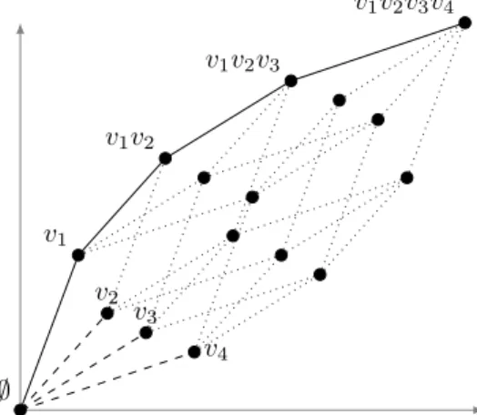
A different algorithm with the same goal was proposed by Breiman et al. [1984] in the context of decision trees, reproduced here as BESTVALUESETCART (Algorithm 4). First, all values are sorted based on their positive/negative ratio. Then the hull is incre-mentally constructed by adding the values one by one in decreasing order with respect to this ratio. For each intermediate value set, the quality of the corresponding feature is computed, and in the end the best one is reported. Note that this only constructs the upper part of the convex hull; the lower part is analogously formed by considering the values in increasing order. The upper hull thus forms a chain, and the lower hull consists of the upper hull’s complements. Therefore, for symmetric quality measures computing the lower convex hull is redundant.
It is easy to see that due to the sorting step the computational complexity of the BESTVALUESETCART algorithm isO(N+dlogd). For attributes with a large domain, that is, withd=O(N), the time complexity can approachO(NlogN). We point out
Algorithm 3:BESTVALUESET(A,ϕ)
Input: nominal attributeA, convex quality measureϕ
Output: value setV ⊆dom(A)maximizingϕ(A∈V)
1 Vmax←dom(A)
2 ϕmax←ϕ(Vmax)
3 foreachvaluevindom(A)do
4 compute stamp pointnvofA=v
5 k←log|dom(A)| 6 for`= 1to2kdo 7 H`k={nv`} 8 whilek≥1do 9 for`= 1to2k−1do 10 computeH`k−1=H H2`k ⊕H2`+1k 11 k←k−1 12 foreachV inH10do 13 ifϕ(V)> ϕmaxthen 14 Vmax←V 15 ϕmax←ϕ(V) 16 returnVmax
Algorithm 4:BESTVALUESETCART(A,ϕ)
Input: nominal attributeA, convex quality measureϕ
Output: value setV ⊆dom(A)maximizingϕ(A∈V)
1 Vmax←dom(A)
2 ϕmax←ϕ(Vmax)
3 foreachvaluevindom(A)do
4 computen+ v, n−v forA=v 5 V←Sn+ v/n−v v0 |n+v0/nv−0 =n+v/n−v 6 V0 ← ∅ 7 (n+, n−)←(0,0) 8 foreachV inVdecreasing w.r.t.n+V/n−V do 9 V0 ←V0∪V 10 (n+, n−)←(n++n+V, n−+n−V) 11 ifϕ(n+, n−)> ϕmaxthen 12 Vmax←V0 13 ϕmax←ϕ(n+, n−) 14 returnVmax
that a straightforward optimization can be applied, by noting that we do not need to check degenerate points on the convex hull. Thus, rather than checking all valuesv individually, we can group all values with the same ration+
v/n−v (line 5). For larged, it is
quite likely that several values have the same ratio, and hence this can reduce the number of evaluations (lines 8–13). More importantly, when sorting, the relative order of values
∅ v1 v2 v3 v4 v1v2 v1v2v3 v1v2v3v4
Figure 4. Illustration of the BESTVALUESETCART algorithm, ford= 4. The upper convex hull (full lines) is constructed by incrementally adding the individual lines sorted by their angle (dashed lines).
with the same ratio is irrelevant. With this observation, we prove that the algorithm can be made to run in linear time, by using a sorting algorithm that properly takes duplicates into account. The basic idea is that even for larged, sorting is always bounded byO(N).
Property 9. The BESTVALUESETCART algorithm can be implemented to run in
O(N+d)time.
Proof. Let us consider the set of alldistinctpositive/negative ratios
ρ=n+v/n−v |v∈dom(A) , (25)
and the empirical distributionµoverρ, defined as µ(r) =
v|n+v/n−v =r /d (26)
forr∈ρ. A sorting algorithm that properly deals with duplicates takesO(η)time per entry on average, where
η=−X
r
µ(r) logµ(r) (27)
is the entropy of its input data [Sedgewick and Bentley, 2002]. We will show that d·η ∈O(N), that is, the complexity of sorting is bounded by the number of examples. Letδ=|ρ| ≤d, and writea=d/δ. Now, the entropyηis maximized ifµis the uniform distribution, i.e., ifµ(r) = 1/δfor all ratiosr, and there areavalues for each distinct ratio. Property 2 tells us that in the worst caseδ∈O (N/a)2/3
, as such we find that d·η≤d·logδ∈Oa(N/a)2/3log(N/a)2/3=O(N) . (28) Hence, the total time complexity of the algorithm isO(N+d).
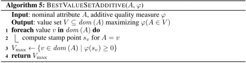
Algorithm 5:BESTVALUESETADDITIVE(A,ϕ)
Input: nominal attributeA, additive quality measureϕ
Output: value setV ⊆dom(A)maximizingϕ(A∈V)
1 foreachvaluevindom(A)do
2 compute stamp pointsvforA=v
3 Vmax← {v∈dom(A)|ϕ(sv)≥0}
4 returnVmax
6.2. Algorithm for Additive Quality Measures
Algorithm 5 can be seen as a simplification of Algorithm 4 for an additive quality measure. Using the additivity ofϕ, the following property shows that updating a value setV with a valuevhaving a positive quality, increases the total quality.
Property 10. LetV ⊆dom(A)andv∈dom(A)withv /∈V. Ifϕ(A=v)≥0then
ϕ(A∈V ∪ {v})≥ϕ(A∈V).
Equality holds if and only ifϕ(A=v) = 0.
Proof. Follows directly from the additivity ofϕ.
Therefore, it is not necessary to construct and check the entire convex hull. Instead, we can directly construct the optimum: the value set that maximizesϕis the union of all attribute values with non-negative quality.
Property 11. The time complexity of BESTVALUESETADDITIVEisO(N+d).
7. Experimental Evaluation
In this section, we demonstrate the efficiency of the presented algorithms, furthermore show that using a richer pattern language results in subgroups of higher quality, and present results on a real-world medical insurance dataset.
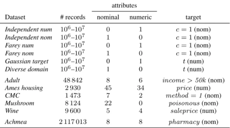
Table 1 presents the characteristics of the datasets we used. The last column shows which attribute is the target, and whether it is nominal or numeric. We created six synthetic datasets and used five publicly available benchmark datasets. TheIndependent
num andIndependent nom datasets consists of one numeric (respectively nominal)
attribute and an independent binary targetc, with probability 50%. The values of the numeric attribute are all distinct, the domain of the nominal attribute is of sizeN/103.
TheFarey numandFarey nomdatasets both correspond to the worst case convex hull,
proportional toN2/3; in the numeric case, this is the number of (non-pruneable) split
points, in the nominal case, this is the domain size. TheGaussian targetdataset has a numeric attributeAwith domain[0,10], and a numeric target that equalsN(5,1)(A).
TheDiverse domaindataset has a nominal attribute with a domain that grows linearly
with N, where the target mean (ranging between 0 and 10) of valuevi is a linear
function ofi, with standard deviation 1. For each type of synthetic dataset, we generated instances with sizes ranging between106and107. The benchmark datasets we used
are the following. TheAmes housingdataset is available from the Journal of Statistics Education data archive [De Cock, 2011]. From the UCI ML Repository we used the
Table 1. Main characteristics of the synthetic, benchmark, and real-world datasets used in the experiments. Shown are the number of recordsN, the number of nominal and numeric attributes, and the target.
attributes
Dataset # records nominal numeric target
Independent num 106–107 0 1 c= 1(nom)
Independent nom 106–107 1 0 c= 1(nom)
Farey num 106–107 0 1 c= 1(nom)
Farey nom 106–107 1 0 c= 1(nom)
Gaussian target 106–107 0 1 t(num)
Diverse domain 106–107 1 0 t(num)
Adult 48 842 8 6 income>50k(nom)
Ames housing 2 930 45 34 price(num)
CMC 1 473 7 2 method=1(nom)
Mushroom 8 124 22 0 poisonous(nom)
Wine 9 600 5 4 saleprice(num)
Achmea 2 117 013 8 8 pharmacy(nom)
dataset is composed of observations derived from 10 years of tasting ratings reported in the Wine Spectator Magazine [Costanigro et al., 2009].
We integrated the algorithms into the open-source subgroup discovery tool Cor-tana [Meeng and Knobbe, 2011].2All experiments were executed on a system with a
2.4GHz dual quad core processor and 24GB of memory, running Linux. For the synthetic datasets, the minimum support threshold was set to 1. For each benchmark dataset, a minimum support of 1% and maximum refinement depth of 3 were used, the search strategy was beam search with a beam width of 100. The multi-threading option of Cortana was not used.
7.1. Performance
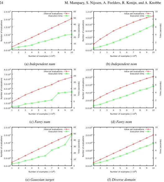
Figure 5 shows the results of performance experiments with the BESTINTERVALand BESTVALUESETalgorithms on the synthetic datasets. We measure the number of feature evaluations and the execution time (excluding reading the data) of each algorithm, as a function of the number of dataset records. The quality measures we used are Information Gain for nominal targets, and standardizedz-score for numeric targets. For numeric attributes, all values occurring in the data were used as candidate split points. The reported execution times are averaged over three runs per dataset.
First, note that the algorithms can handle datasets with millions of records in just a few seconds, and even for the largest datasets require less than a minute. The number of considered features (intervals or value sets) grows at most linearly with respect to dataset size in all figures. In particular, the number of evaluations in Figures 5b and 5d grow slightly sublinearly, in accordance with Property 2. Further, we see that the execution times scale proportionally to the number of feature evaluations, and linearly in the number of examples.
0.0⋅100 5.0⋅106 1.0⋅107 1.5⋅107 2.0⋅107 2.5⋅107 1 2 3 4 5 6 7 8 9 10 0 10 20 30 40 50 60 Number of evaluations Time (seconds) Number of examples (×106) Interval evaluations Execution time
(a)Independent num
0.0⋅100 2.0⋅103 4.0⋅103 6.0⋅103 8.0⋅103 1.0⋅104 1.2⋅104 1 2 3 4 5 6 7 8 9 10 0 2 4 6 8 10 Number of evaluations Time (seconds) Number of examples (×106)
Value set evaluations Execution time (b)Independent nom 0.0⋅100 1.0⋅105 2.0⋅105 3.0⋅105 4.0⋅105 5.0⋅105 6.0⋅105 7.0⋅105 8.0⋅105 1 2 3 4 5 6 7 8 9 10 0 5 10 15 20 25 30 Number of evaluations Time (seconds) Number of examples (×106) Interval evaluations Execution time (c)Farey num 0.0⋅100 2.0⋅104 4.0⋅104 6.0⋅104 8.0⋅104 1.0⋅105 1 2 3 4 5 6 7 8 9 10 0 2 4 6 8 10 Number of evaluations Time (seconds) Number of examples (×106) Value set evaluations
Execution time (d)Farey nom 0.0⋅100 5.0⋅106 1.0⋅107 1.5⋅107 2.0⋅107 2.5⋅107 1 2 3 4 5 6 7 8 9 10 0 10 20 30 40 50 60 Number of evaluations Time (seconds) Number of examples (×106) Interval evaluations Execution time
(e)Gaussian target
0.0⋅100 5.0⋅103 1.0⋅104 1.5⋅104 2.0⋅104 2.5⋅104 1 2 3 4 5 6 7 8 9 10 0 2 4 6 8 10 Number of evaluations Time (seconds) Number of examples (×106) Value set evaluations
Execution time
(f)Diverse domain
Figure 5. Number of feature evaluations and execution times in seconds of the BESTIN
-TERVALand BESTVALUESETalgorithms as a function of the number of dataset records, for the synthetically generated datasets.
7.2. Quality
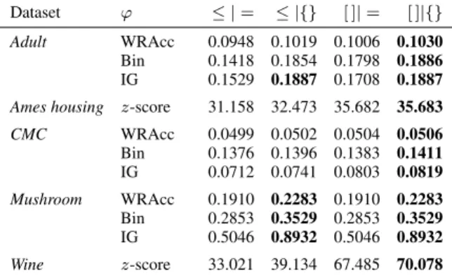
Table 2 contains the results of qualitative experiments on the benchmark datasets, for several quality measures. We run the Cortana subgroup discovery tool for several quality measures, using beam search with a beam width of 100 and a maximal search depth of 3. We calculate the average quality of the top 10 subgroups, allowing different types of feature descriptions for nominal and numeric attributes, that is, standard equalities and inequalities, value sets instead of single values, intervals instead of inequalities, and both value sets and intervals. As to be expected, the table shows that using intervals or value sets as descriptions increases the average quality of the discovered subgroups, whereas using both types of descriptions increases average subgroup quality the most. This is a
Table 2. Average score of the top 10 discovered subgroups using either standard de-scriptions (equalities and inequalities), value sets, intervals, or both, for various quality measures, with minimum support=1%, search depth=3, and beam width=100.
Dataset ϕ ≤ |= ≤ |{} [ ]|= [ ]|{} Adult WRAcc 0.0948 0.1019 0.1006 0.1030
Bin 0.1418 0.1854 0.1798 0.1886
IG 0.1529 0.1887 0.1708 0.1887 Ames housing z-score 31.158 32.473 35.682 35.683 CMC WRAcc 0.0499 0.0502 0.0504 0.0506 Bin 0.1376 0.1396 0.1383 0.1411 IG 0.0712 0.0741 0.0803 0.0819 Mushroom WRAcc 0.1910 0.2283 0.1910 0.2283 Bin 0.2853 0.3529 0.2853 0.3529 IG 0.5046 0.8932 0.5046 0.8932 Wine z-score 33.021 39.134 67.485 70.078
direct result of an increased feature search space, allowing for higher quality subgroups to be discovered.
7.3. Real-World Demonstration
We describe an application of our methods to the field of fraud detection in a medical insurance dataset, obtained from Achmea, the largest health insurance company in the Netherlands. We aim to illustrate the value of the proposed extension in expressive power, and additionally demonstrate that a scalable solution has been achieved that provides accurate results on large data, in an interactive setting. The results pertain to a dataset describing pharmacies. In total, some 2.1 million records of individual medication are available, involving 100 pharmacies: one pharmacy under investigation and 99 of its peers (comparable pharmacies). A total of 16 attributes, both nominal and numeric, describe each prescription, and an additional binary target indicates the pharmacy under investigation. This pharmacy contributes 11 380 records (0.54%) to the dataset. The attributes provide information about the patient involved, such as their birth date and gender, as well as various pharmaceutical categories and the dosage and amount of medication. With the aim of characterizing deviating claim behaviour at this pharmacy, and potentially understanding population differences at this pharmacy, we look for interesting subgroups using Cortana, including the extensions described in this article.
For the WRAcc measure, some interesting individual conditions found were as follows:
number of pieces∈]29,204]
day of the week∈ {Monday, Tuesday, Thursday}
These conditions cover roughly 1.5 and 1.2 million examples, respectively. A more specific and accurate result, discovered at depthd= 2is as follows:
cost∈]8.69,512.12]∧date of birth∈]December 18, 1916, June 24, 1959]
This result, which covers about a million records with a target share of 0.87%, demon-strates nicely how our method finds the optimal boundaries of intervals with much detail, and furthermore does so in a dynamic fashion: the optimal birth dates were computed on
the subset of records that satisfy the first condition. A similar result involving value sets is as follows:
delivery-code∈ {1,3,4,5,10,11,15,16,20,21} ∧cost∈]7.49,512.12]
The 10 codes, out of a total of 20, describe several legal regulations concerning compen-sation for complicated preparation, delivery at night, and so on. The codes in this value set all relate to delivery during regular office hours, as opposed to the codes for evenings, nights and Sundays.
The data also includes attributes of the Anatomical Therapeutic Chemical Classifi-cation (ATC) system, which is a multi-level classifiClassifi-cation of drugs. Theses attributes, providing different levels of the ATC hierarchy, tend to produce large value sets of possibly hundreds of codes. Although such value sets may be interesting to the expert, they do not necessarily represent high-level insight into the domain. For this reason, we have excluded nominal attributes with cardinalities above 100.
Despite the size of the dataset and the numeric data involved, producing a set of subgroups at depthd= 2took only 12 seconds; a depthd= 3run took 50 seconds. A minimum coverage of 1 000 records and a beam-width of 100 were used.
8. Conclusions
We presented efficient algorithms for finding optimal binary features in labeled data with respect to a convex quality measure. These features have descriptions in the form of intervals for numeric attributes, and value sets for nominal attributes. By directly constructing the convex hull of the set of all feature stamp points in coverage space, we can disregard vast portions of the search space. We presented some general theoretical properties of convex hulls in coverage spaces, and showed that in the important case of a binary target, the time complexity of the presented algorithms is linear in the number of examples. Experiments on synthetic, benchmark, and real-world data, demonstrated that as such, even for large datasets we can efficiently discover high quality features with rich descriptions.
Acknowledgements
This research is partially supported by the Netherlands Organization for Scientific Research (NWO) under project nr. 612.065.822 (Exceptional Model Mining), and by a Postdoc grant from the Research Foundation—Flanders (FWO).
References
Rakesh Agrawal, Tomasz Imielinski, and Arun Swami. Mining association rules be-tween sets of items in large databases. InProceedings of the 1993 ACM SIGMOD
international conference on management of data, pages 207–216, 1993.
Martin Atzm¨uller and Frank Puppe. SD-Map–A fast algorithm for exhaustive subgroup discovery. InProceedings of PKDD, pages 6–17, 2006.
Leo Breiman, Jerome Friedman, Charles J. Stone, and Richard A. Olshen.Classification