Widescale analysis of transcriptomics data using cloud computing methods

(1)

Widescale analysis of transcriptomics

data using cloud computing methods

Anne M. Owen

A thesis submitted for the degree of

Doctor of Philosophy (Ph.D.)

Department of Mathematical Sciences

University of Essex

(2)

Dedicated to

(3)

Acknowledgements

I am extremely grateful to my supervisor, Dr Andrew P. Harrison, for his inspiration and encouragement throughout the period of study for this degree. For many years I had wondered if I would be able to achieve the level of study required for a doctorate, having rejected the opportunities I was offered at age 23. Harry saw some potential and had faith in me at this later stage in my career. He has guided the research, read many chapter drafts and advised on the shape of the thesis.

My grateful thanks also go to Dr Adrian Clark of the Computing Science and Electrical Engineering Department of the University of Essex for backing up Harry as my second supervisor. Adrian enabled me to present to his Masters students about Cloud Computing and made very helpful comments on the draft thesis.

I would like to thank Dr Hugh P. Shanahan of Royal Holloway College, London Uni-versity, for his collaboration and help during work on the Windows Azure Cloud, for his part in developing GWydiR and for his comments on reading some of the thesis chapters. My thanks also go to Prof. Graham Upton for his helpful statistical insights. Ibrahim Musa has been an inspiring collaborator in the work on a local cloud, and I am grateful for his enthusiastic support. Farhat Memon was a great encouragement as a fellow PhD student in Bioinformatics, and indeed it was while helping her to work on the Amazon cloud that the possibility of my study was suggested.

I am grateful for the R scripts used by Hugh Shanahan and Farhat Memon in their research into G-stacks as these formed the basis of the scripts used in the wide scale survey

(4)

iv

work.

My husband, Peter, has been a tower of strength and support throughout my journey. He has made sacrifices in many ways. Above all I give glory to God who helped me start, progress and finish this thesis. He was my strength through many times of doubt and weakness.

(5)

Summary

This study explores the handling and analyzing of big data in the field of bioinformatics. The focus has been on improving the analysis of public domain data for Affymetrix GeneChips which are a widely used technology for measuring gene expression. Methods to determine the bias in gene expression due to G-stacks associated with runs of guanine in probes have been explored via the use of a grid and various types of cloud computing.

An attempt has been made to find the best way of storing and analyzing big data used in bioinformatics. A grid and various types of cloud computing have been employed. The experience gained in using a grid and different clouds has been reported. In the case of Windows Azure, a public cloud has been employed in a new way to demonstrate the use of the R statistical language for research in bioinformatics.

This work has studied the G-stack bias in a broad range of GeneChip data from public repositories. A wide scale survey has been carried out to determine the extent of the G-stack bias in four different chips across three different species. The study commenced with the human GeneChip HG U133A. A second human GeneChip HG U133 Plus2 was then examined, followed by a plant chip, Arabidopsis thaliana, and then a bacterium chip, Pseudomonas aeruginosa. Comparisons have also been made between the use of widely recognised algorithms RMA and PLIER for the normalization stage of extracting gene expression from GeneChip data.

(6)

Declaration

The study presented in this thesis is all my own work, except where otherwise stated and acknowledged. It has not already been accepted for any degree and is also not being concurrently submitted for any other degree.

(7)

Glossary

amino acidsare biologically important organic compounds composed of amine (N H2) and

carboxylic (COOH) functional groups, together with a side-chain specific to each amino acid. Their key elements are carbon, hydrogen, oxygen and nitrogen. About 500 amino acids are known.

cytoplasm is a gel-like substance enclosed within a cell’s membrane. Most cellular activities occur within the cytoplasm.

enzymesare highly selective catalysts which are responsible for the thousands of meta-bolic processes that sustain life. Most enzymes are proteins, though some catalytic RNA molecules have been identified.

G-stackis a sequence of four “G” (guanine) bases in a strand of nucleic acid such as RNA or DNA.

gene productis the biochemical material, either RNA or protein, which results from expression of a gene.

hybridization is the process of joining two complementary strands of nucleic acid sequences, e.g. RNA or DNA.

microarrayis a 2D array on a glass slide for testing biological material using hibridiza-tion and laser scanning.

nucleic acidsare large biological molecules which are essential for all known forms of life. DNA and RNA are examples. They encode, transmit and express genetic information.

(8)

viii nucleotides are the building blocks of nucleic acids like DNA and RNA. They are composed of a nitrogenous base with a five-carbon sugar and at least one phosphate group.

polymersare large molecules which are composed of many repeated subunits. Polymers range from familiar synthetic plastics like polystyrene to natural biopolymers like DNA and proteins.

photolithography is a process that uses light to control the manufacture of multiple layers of material.

polypeptidesare long continuous chains of amino acids. In general they are smaller than proteins so have fewer amino acids (approximately 50 or fewer according to Wiki).

probe affinity(a description used by Irizarryet al.[1]) is the attraction which causes hybridization of strands of nucleic acid sequences. Abnormal probe affinity relates to a probe sequence having an affinity to bind to a neighbouring probe rather than to the desired RNA sequence. Affymetrix, to be strictly accurate, prefers to use the term “feature responses” in place of “probe affinities” due to the many factors which interact to produce measured intensity [2].

proteinsconsist of one or more polypeptides, arranged in a biologically functional way.

web roleis a web application which is accessible via ahttp://... orhttps://... endpoint (webpage or web address)

(9)

List of Figures

2.1 Structure of Prokaryote Cells. (Source: Shmoop Biology

http://www.shmoop-.com/biologycells/prokaryoticcells.html) [Accessed April 8, 2014] . . . . 8

2.2 Comparison of Eukaryotic Animal and Plant Cells (Source: The Ponder-ing Gulch

http://www.theponderinggulch.com/2011/07/frontyard-senseback-yard-science-getting.html) [Accessed April 29, 2014] . . . 9

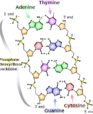
2.3 Similarities and Differences between DNA and RNA. (Source: Wikimedia Commons) [Accessed April 29, 2014] . . . 10 2.4 Chemical structure of DNA. Hydrogen bonds are shown by dotted lines.

(Source: Wikipediahttp://en.wikipedia.org/wiki/DNA) [Accessed April 29, 2014] . . . 11 2.5 The Central Dogma of Molecular Biology with Enzymes. (Source:

Wiki-pedia) [Accessed April 29, 2014] . . . 12 2.6 Exons and Introns (Source: The National Human Genome Research

In-stitute http://www.genome.gov/Images/EdKit/bio2i large.gif) [Accessed November 6th, 2013] . . . 14 2.7 Alternative Splicing (Source: The National Human Genome Research

Institute http://www.genome.gov/Images/EdKit/bio2j large.gif) [Accessed June 23, 2014] . . . 15 2.8 A Grid systems taxonomy . . . 24

(18)

List of Figures xviii

2.9 Simplified explanations for the three main layers of cloud computing ( http:-//venturebeat.com/2011/11/14/cloud-iaas-paas-saas/) [Accessed September 17th, 2014] . . . 33

3.1 An Affymetrix GeneChip®(Source:

https://www.flickr.com/photos/jseita/-3764113525) [Accessed February 20, 2015] . . . 38

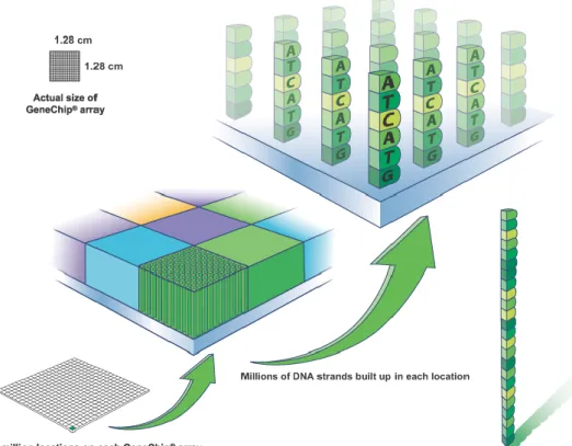
3.2 The small quartz wafer microarray contains thousands of 25-mer probes in each tiny square of its array (Courtesy of Affymetrix, Inc., Santa Clara, CA,

USA

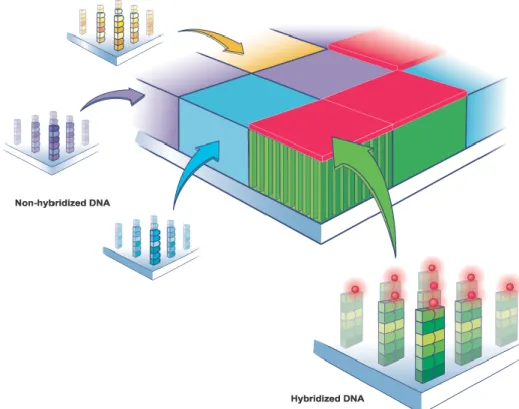
http://media.affymetrix.com/media/corporate/media/imagelibrary/high-res/singlefeature.zip) [Accessed April 9, 2014] . . . 39 3.3 Affymetrix GeneChip Hybridization: fragments of RNA stick to the probes

(Courtesy of Affymetrix, Inc., Santa Clara, CA, USA

http://media.affymetrix.-com/media/corporate/media/imagelibrary/highres/hybridizationoftag-gedprobes.zip) [Accessed April 9, 2014] . . . 40 3.4 Hybridized DNA fragments glow when a laser light is shined on to a

microar-ray, which contains many millions of fragments (Courtesy of Affymetrix, Inc., Santa Clara, CA, USA

http://media.affymetrix.com/media/corporate/-media/imagelibrary/highres/taggedanduntagged.zip) [Accessed April 9th,

2014] . . . 41 3.5 Rankings of selected methods on 14 outcomes, from the Affycomp website 52 3.6 Comparison of Bias in four selected probe summary methods at different

concentrations for U133 data . . . 53 3.7 Scatter diagram comparing probe pm6 from probe set 31846 at with probe

pm1 from probe set 219297 at (Source: Uptonet al.[12]) . . . 57 3.8 Correlation matrix showing the correlation coefficients between every pair

of the 16 perfect match probes that form the 31846 at probe set (Source: Uptonet al.[12]) . . . 58

(19)

List of Figures xix

3.9 Schematic of a G-tetrad and G-quadruplexes. (a) Four guanine (G) residues can form a planar structure, termed a G-tetrad, through Hoogsteen hydrogen bonding. (b) A tetramolecular parallel G-quadruplex can be formed from four DNA strands each with a single G-rich repeat. (c) DNA sequences that contain two or more G-rich repeats can form GG hairpins, which in turn dimerize to form several types of stable bimolecular quadruplexes, termed intermolecular antiparallel G-quadruplexes. (d) DNA sequences with either four G-rich repeats or long G tracts can fold upon themselves to form an antiparallel intramolecular quadruplex, termed an intramolecular foldover G-quadruplex. (Source: Han and Hurley [54]) . . . 60 3.10 Bar chart of the average correlation between G-stack probes (in blue) and

C-stack probes (in red) for 176 HG U133A GeneChip experiments deposited at GEO. . . 63 3.11 Bar chart of the average correlation between G-stack and C-stack probes

for 176 HG U133A GeneChip experiments deposited at GEO. Reproduced from the paper by Shanahanet al.[38] . . . 63 3.12 HG U133A expression estimates showing median differences when

C-stacks and G-C-stacks are removed respectively . . . 65 3.13 HG U133A GT correlation data for median differences of C-stacks and

G-stacks present and removed respectively . . . 67 3.14 HG U133A LT correlation data for median differences of C-stacks and

G-stacks present and removed removed respectively . . . 68

5.1 Flow within Amazon Elastic Compute Cloud (Source: Amazon documenta-tion fromhttp://aws.amazon.com/) . . . 85 5.2 Some of the Amazon EC2 services available to an application or a machine

instance (Source:

(20)

List of Figures xx

5.3 Framework and interaction of components in the proposed virtual infras-tructure containerhttp://www.journalofcloudcomputing.com/content/3/1/5

[Accessed September 29th, 2014] . . . 88 5.4 Elements of Azure (

http://solutions.devx.com/ms/developer-cloud/migra-ting/introducing-the-azure-services-platform-46874.html) [Accessed Octo-ber 14th, 2014] . . . 93 5.5 The three types of storage that Azure provides

(http://sijinjoseph.com/2008-/11/14/windows-azure-distilled/)[Accessed October 14th, 2014] . . . 94

6.1 Simple flow representation of Windows Azure (http://sijinjoseph.com/2008-/11/14/windows-azure-distilled/)[Accessed October 14th, 2014] . . . 101 6.2 Screenshot of webpage used to launch an R script . . . 103 6.3 Functionality of the Generic Worker (GW) (Source: Early Venus-C

docu-mentation) . . . 104 6.4 Design flow of Generic Worker web role (Source: Early Venus-C

documen-tation) . . . 105 6.5 The use of GWydiR with Azure . . . 107 6.6 Time taken to load microarray data from Azure mass storage to R working

storage. Plot shows the time in seconds taken to load each of 576 datasets from Azure blob storage to local VM disk space, in terms of the number of CEL files in each GSE experiment. . . 112 6.7 Time taken to analyze data with R script using Azure. Plot shows the time

in seconds taken to analyze each of 576 datasets, in terms of the number of CEL files in each GSE experiment. . . 113

(21)

List of Figures xxi

6.8 Comparison of analysis times between cloud and two local machines. Plot shows the time in seconds taken to analyze each of six particular experi-ments, in terms of the number of CEL files in each GSE experiment. The particular experiments were chosen because they had 4, 8, 16, 32, 64 and 128 CEL files, to give a range of experiment data amounts. The machine labelled Local1 had a CPU clock speed of 2.13 GHz, and the machine labelled Local2 had a CPU clock speed of 2.24 GHz. The 70% CPU cap was added to the Local2 machine to crudely estimate the slower 1.60 GHz stated clock speed of the Azure VM. . . 114

7.1 Flow of Data Analysis jobs . . . 118 7.2 The average correlation of expression levels for G-stack probes over all

CEL files of the designated experiments, and the number of CEL files in each case, ordered by highest correlation first . . . 120 7.3 Plots of the median differences in GT correlation data (more than 0.4) over

573 HG U133A GSEs, in ranges depending on the number of CEL files in each GSE . . . 123 7.4 Plots showing the length of processing time for RMA compared to PLIER

normalization routines, on experiments with 2, 4, 8, 16, 32, 64, and 128 (approx.) CEL files. The mean of the timing of each group of experiments is shown by a triangle (RMA) and by a square (PLIER). . . 125 7.5 Median differences in correlation values (greater than 0.4) between where

G-stacks were kept in and removed, using RMA and PLIER for all 576 experiments . . . 127 7.6 Comparison of median differences in correlation values (greater than 0.4)

between where G-stacks were kept in and removed, using RMA and PLIER for all 576 experiments. The line of equality is shown. . . 128 7.7 Expression estimates for HG U133A GeneChip . . . 130

(22)

List of Figures xxii

7.8 Correlation differences for HG U133A GeneChip . . . 131

8.1 Scatter Plot of Expression Data for 576 datasets of HG U133A GeneChip 134 8.2 Scatter Plots of Expression Data for 1999 datasets of the HG U133 Plus2

GeneChip . . . 135 8.3 Scatter Plot of Expression Data for 625 datasets of Arabidopsis GeneChip 138 8.4 Scatter Plot of Expression Data for 79 datasets of Pseudomonas GeneChip 138 8.5 Expression Data for HG U133 Plus2 GeneChip . . . 140 8.6 Comparing G-stacks in HG U133A and HG U133 Plus2 GeneChips . . . . 141 8.7 Comparison of GT correlation data for HG U133 Plus2 GeneChip using

RMA and using PLIER . . . 142 8.8 Expression data for Arabidopsis GeneChip . . . 143 8.9 Comparing G-stacks in Arabidopsis GeneChip with those in HGU 133A

and HGU 133 Plus2 GeneChips for expression data . . . 144 8.10 Expression data for Pseudomonas GeneChip . . . 146 8.11 Comparing G-stacks in Pseudomonas and Arabidopsis GeneChips with

those in HGU 133A and HGU 133 Plus2 GeneChips . . . 146 8.12 Comparing median difference in GT correlation data using RMA and using

PLIER . . . 147 8.13 Comparing median difference in GT correlation data for four species using

RMA and using PLIER . . . 149

D.1 Architecture of resource interactions in the private cloud . . . 186 D.2 Result comparing the thrashing rate between the proposed algorithms using

common provisioning algorithms . . . 191 D.3 Result comparing the job makespan between the proposed job allocation

algorithm and other algorithms . . . 194 D.4 Cost comparison among various job allocation algorithms . . . 195

(23)

List of Figures xxiii

E.1 The Venus-C website home page from June, 2012, showing where Biology and Bioinformatics were the subject areas of some of the 15 pilot projects as well as some of the original 7 partner scenarios . . . 197

(24)

List of Tables

3.1 The numbers of probe sets in HG U133A that have particular numbers of G-stack probes . . . 64

4.1 Table of varying execution times for the same job with 6 CEL files, which were run on the NGS Rutherton Appleford laboratory node and on four local machines . . . 80

7.1 The basic descriptive statistics of the GT correlation data for each range of CEL files . . . 123

8.1 Details of the outliers in the scatter plots of HG U133 Plus2. Outliers are listed from the top as labelled clockwise in the plots of Figure 8.2. The capital letters ‘R’ and ‘P’ after the GSE experiment number stand for RMA and PLIER respectively. GSE22132 is an outlier in both the RMA and PLIER plots. . . 136 8.2 Details of the outliers in the scatter plots of Arabidopsis. Outliers are listed

from the top as labelled clockwise in the plots of Figure 8.3. The capital letters ‘R’ and ‘P’ after the GSE experiment number stand for RMA and PLIER respectively. GSE10039 is an outlier in both the RMA and PLIER plots. . . 139 8.3 The numbers of probe sets in Arabidopsis that have particular numbers of

G-stack probes . . . 144

(25)

List of Tables xxv

A.1 File Contents for Version 4 Format CEL files . . . 163

B.1 File Contents for CDF files . . . 169 B.2 File Contents for XDA Format CDF files . . . 172

(26)

Chapter 1 Introduction

The study described in this thesis covers investigations made in the fields of bioinformatics and computer science. It is necessary to understand some biological and chemical structures in order to use bioinformatics and study the data that biologists generate so these structures have been briefly described. Computers are invaluable to perform the desired analyses and also to handle the large volumes of data that can be involved so there are chapters dedicated to explaining the type of computation facilities used.

Much use has been made in recent years of microarray technology to perform research into gene expression and the chemical processes behind cell development. Experiments are also creating vast amounts of sequencing data in a variety of fields where DNA and RNA are of interest. Microarray data has been examined here to establish methods of confirming the bias that can be introduced to this data by the particular probes chosen in the Affymetrix GeneChip® technology (see chapter 3). From the various types of bias that have been detected (for example by Langdonet al.[3] and by Upton and Harrison [4]) the effect of G-stacks (sequences of four or more “G”s) in the probes was chosen to be investigated in more detail. A wide scale survey of all experiments that used a particular human GeneChip has been carried out. This survey was repeated for another human GeneChip, and then for GeneChips in two other species.

An attempt has been made to find a good way of handling and analyzing big data in the

(27)

1.1. Organisation of thesis 2

field of bioinformatics. The use of a grid and of cloud computing is explored to examine the process of investigating large amounts of data from microarray experiments. This type of data is often deposited and made available in public databases accessible across the internet. The use of a local private cloud has been demonstrated and in the case of Windows Azure, a public cloud has been employed in a new way to demonstrate the use of the R statistical language for research in bioinformatics.

Ever increasing quantities of data are being generated each year. This data can be analysed by other researchers from those who created it, in order, for example, to search for patterns of gene expression that might not have been anticipated. This work paves the way for fresh approaches in the handling and analysis of large volumes of biological data of any type.

1.1 Organisation of thesis

Chapter 2introduces the basic principles of molecular biology in terms of the cell, DNA and RNA, genes and the genome, and bioinformatics and its tools. It concludes with an explanation of the challenge presented by “Big Data” in the field of bioinformatics, and with an overview of grid and cloud computing.

Chapter 3explains the use of microarrays and the technology of Affymetrix GeneChips. It explores how gene expression is evaluated from the results of microarray experiments and how bias can be introduced by certain sequences such as G-stacks. This bias is the focus of further analysis described in later chapters. The generation of “unique mappings” is explored and analytic techniques of regression analysis and correlation matrices are explained as a way to evaluate the bias due to G-stacks.

Chapter 4explores grid computing as a solution to the problem of accessing computer resources as a bioinformatician when fast processors and huge storage devices are not available locally. Grid computing is examined through experiences of using the NGS grid

(28)

1.1. Organisation of thesis 3

which was the National Grid Service for the academic research community in the United Kingdom.

Chapter 5contrasts the experiences of using a local private cloud and two public clouds: Amazon Web Services and Microsoft’s Windows Azure. This research project enjoyed early access to both the Amazon and Azure cloud offerings, whose features and advantages have improved and grown enormously over the period.

Chapter 6 explains the experience of using Windows Azure cloud services when they were newly available, to begin to analyse a large quantity of microarray data. The development of bespoke interfaces to run R scripts in the Windows-centric environment of Azure is described. Data sets had to be uploaded from public repositories of microarray experiments. Finally some timings of running R scripts in the cloud is compared with timings on local computers.

Chapter 7 returns to the biological experiment data from microarrays to report on the experience of using the Azure cloud to analyse all the publicly available data from the human GeneChip HG U133A. There are issues to be discussed when uploading large quantities of data from many experiments of different researchers. There was also the need to develop a new method of submitting multiple jobs to analyse the data. This work allowed the assessment of the extent of G-stack bias across a wide variety of experiments which used the HG U133A chip.

Chapter 8extends the wide scale analysis to another human GeneChip HG U133 Plus and to two other species: the plantArabidopsis thalianaand the bacteriumPseudomonas aeruginosa. Scatter plots are used to compare the results in each species between using RMA and PLIER, two different types of normalization routine. Expression data and correlation data across probe sets are both used to compare the effects of G-stacks in the probes of the microarray datasets of each species.

Chapter 9summarises the conclusions of the thesis. It also suggests ways in which future research might profitably be directed.

(29)

1.2. Published papers 4

1.2 Published papers

1. Musa, Ibrahim K., Owen, Anne M., Harrison, Andrew P. and Walker, Stuart D. (May 2014) Self-service infrastructure container for data intensive application.Journal of Cloud Computing: Advances, Systems and Applications, vol. 3, no. 1

2. Shanahan, Hugh P., Owen, Anne M., Harrison, Andrew P. (Jan 2014) Bioinformatics on the cloud computing platform Azure. PloS One 9.7 ISSN: 1932-6203. URL: http://dx.plos.org/10.1371/journal.pone.0102642

3. Shanahan, Hugh P., Owen, Anne M., Harrison, Andrew P. (July 2013) Integrating R with a Platform as a Service cloud computing platform for Bioinformatics applications.

The R User Conference, useR! 2013, Book of Contributed Abstractspage 7 URL:

http://www.edii.uclm.es/ useR-2013/abstracts/files/150 HughShanahanAzure.pdf

4. Memon, Farhat N., Owen, Anne M., Sanchez-Graillet, Olivia, Upton, Graham J.G., and Harrison, Andrew P. (2010) Identifying the impact of G-Quadruplexes on Affy-metrix30 Arrays using Cloud Computing. Journal of Integrative Bioinformatics, vol. 7, no. 2, 111

5. Memon, Farhat N., Sanchez-Graillet, Olivia, Upton, Graham J.G., Owen, Anne M., and Harrison, Andrew P. (2009) Identifying the impact of G-Quadruplexes on Affymetrix exon arrays using cloud computing. CIB2009 URL: http://www. cls.zju.edu.cn/binfo/IB/2009/Proceeding.pdf#page=55.

1.3 My contribution

My contribution to the field of Bioinformatics through this thesis is the wide scale analysis of publicly available transcriptomics data, the results of which are given in detail in chapters 7 and 8. In order to achieve these results all possible microarray data from four different

(30)

1.3. My contribution 5

GeneChips that was available in May 2012, was uploaded to a public cloud and analysed. The types of analysis chosen were based on work by Shanahan and Memon which is described in section 3.5. I modified their scripts to run on the Azure cloud.

Initially I was involved with my supervisor’s team of researchers in creating unique mappings (see section 3.4.2) which identified probes that could be used as more reliable mea-sures of target expression. Following this was the creation of heatmaps (see section 3.4.3.2) which visualize the correlation coefficients between pairs of probes in a probe set. The heatmaps showed that some probes were not correlated with other probes in their probe sets, and yet probes containing runs of guanine typically showed correlation with each other. The investigation of runs of guanine was showing them to be a cause of error or bias in measuring gene expression. I do not believe that there had ever been a wide scale survey done to find out the magnitude of this bias across all the available experimental data deposited in public databases.

Computing grids had been in use for several years but computing clouds were in their infancy, so with my background in computing science (M.Sc. Newcastle, 1973 as Anne Yates), I embarked on the use of a grid and cloud computing to perform the analysis runs. The experiences reported on using grid computing were with a script written by Farhat Memon. My experience on the Amazon cloud came initially from helping Farhat to get started with cloud computing. I was able to create some tailored machine images for her to use for our group research. I also uploaded and maintained data files in Amazon S3 storage.

My personal contribution to the work on Musa’s local private cloud was firstly to supply the same data and R scripts that I was using to analyse the effect of runs of guanines. Then discussion of the bioinformatics issues as well as the cloud job queuing issues ensured that Musa and I both gained the maximum benefit from the collaboration.

The wide scale analyses were run on the Windows Azure cloud. I modified scripts written in R by Shanahan and Memon to run the analyses. I wrote the C# code necessary to launch web roles on the cloud, as described in section 5.3.2. I wrote scripts to upload data

(31)

1.3. My contribution 6

files from public databases to the Azure cloud storage, ran these scripts to upload data from around 3,000 experiments and ran the various R scripts on the cloud.

(32)

Chapter 2 Basic Principles of Molecular Biology,

Bioinformatics, Big data, Grids and

Clouds

2.1 Introduction

In this chapter an explanation is given of the current basic understanding of the building blocks of life. Starting with the cell as an important functional unit of life, an explanation of DNA (or DeoxyriboNucleic Acid) and some of the mechanisms used in the replication of cells is presented. Section 2.4 will introduce the Central Dogma of Molecular Biology, RNA (RiboNucleic Acid) and amino acids, before explaining what is referred to as a genome. Gene expression is briefly introduced and then an explanation of exons and introns will lead on to an introduction of the field of bioinformatics and some of its tools. The chapter will conclude with a summary of the scale of the big data challenge which faces researchers in bioinformatics today, and outline the basic features of grid computing and cloud computing which have developed to meet the needs of such a challenge.

(33)

2.2. The Cell 8

2.2 The Cell

The number of living species on the earth today is thought to be5±3million [5] of which 1.5 million are named. Each species is different, and the members of each one are capable of reproducing themselves. Many living organisms are single cells. Others, such as human beings, comprise many groups of cells which perform specialized functions, and are linked by intricate systems of communication. Whether made of one cell or many million cells, each organism is generated from a single cell originally. This single cell contains hereditary information that defines the species. It also contains the machinery to construct a new cell which is a complete copy of itself.

Figure 2.1: Structure of Prokaryote Cells. (Source: Shmoop Biology

http://www.shmoop-.com/biologycells/prokaryoticcells.html) [Accessed April 8, 2014]

Bacteria, who do not have a nucleus in their cells, are calledprokaryote cells. Other organisms like mammals, plants and fungi, whose cells are more complex and contain nuclei, are calledeukaryotes. Figure 2.1 shows some details of typical prokaryote cells. The prokaryote cells of bacteria and archaea which are both microscopic organisms usually shaped like rods or spheres, have only one compartment in the cell. It contains DNA, usually in a single circular chromosome.

(34)

2.3. DNA 9

Eukaryotic cells, by contrast, are found in many shapes and sizes. They are larger than prokaryotic cells. DNA is stored in the nucleus of eukaryotic cells, in (usually) multiple linear chromosomes with a more complicated gene structure than for prokaryotic cells. Figure 2.2 shows a stylized diagram of typical eukaryotic cells for both plant and animal examples. In both cases the DNA stored within the nucleus is there to give precise information for the replication of cells and for the development of complete living organisms. The work in this thesis concentrates mainly on eukaryotic cells though in Chapter 8 where a wide scale comparison of the data on four different species is described, the bacterium

Pseudomonas aeruginosais included as an example prokaryote.

Figure 2.2: Comparison of Eukaryotic Animal and Plant Cells (Source: The Pondering Gulch

http://www.theponderinggulch.com/2011/07/frontyard-senseback-yard-science-getting.html)

[Ac-cessed April 29, 2014]

2.3 DNA

The building blocks of DNA and RNA are shown in Figure 2.3, with details of the bonding of the bases of DNA shown in Figure 2.4. DNA is a double-stranded molecule where each strand consists of a sequence ofnucleotides. Each nucleotide consists of three parts: a

(35)

2.3. DNA 10

Figure 2.3:Similarities and Differences between DNA and RNA. (Source: Wikimedia Commons) [Accessed April 29, 2014]

sugar(deoxyribose) part attached to aphosphatepart, and abaseof either adenine (A), cytosine (C), guanine (G) or thymine (T), so that an example sequence might be GAATTC... The pairing rule of DNA is that A pairs with T and C pairs with G. So in double-stranded form the six base pairs in the example

are:-The nucleobases in Figure 2.3 are referred to asnitrogenous basesas they are rich in nitrogen atoms. It can be seen in Figure 2.4 that they hold together across the two strands with hydrogen bonds. The figure shows that adenine and thymine form two hydrogen bonds between them which is represented asA=T orT =A. Guanine and cytosine form three hydrogen bonds between them, written as G ≡ C or C ≡ G. These two base pairings between A & T and between G & C are known as Watson-Crick base pairs and are crucial

(36)

2.3. DNA 11

Figure 2.4: Chemical structure of DNA. Hydrogen bonds are shown by dotted lines. (Source: Wikipediahttp://en.wikipedia.org/wiki/DNA) [Accessed April 29, 2014]

for the DNA double helix structure formation, pictured in Figure 2.3.

In Figure 2.4 the groups of four oxygen (O) atoms with phosphate (P) in the centre are phosphate groups and the pentagons with four carbon (C) atoms and an oxygen atom are deoxyribose (sugar). The sugar part of each DNA molecule binds to the next phosphate part with a covalent bond. This strong sugar-phosphate linkage has led to these two strand parts of DNA being known as the ‘backbone’. It should be noted that the sugar-phosphate backbone always gives a direction or polarity to the strand, and that the two ends of a single strand are known as the “30end” and the “50 end”. 30(3 prime) represents the carbon atom in the sugar to which the next phosphate or50 (5 prime) end of the adjacent base attaches. The information in DNA is read and/or copied through the direction from the50 end to the

(37)

2.4. Central Dogma of Molecular Biology 12

Figure 2.5: The Central Dogma of Molecular Biology with Enzymes. (Source: Wiki-pedia) [Accessed April 29, 2014]

2.4 Central Dogma of Molecular Biology

Thecentral dogma of molecular biologyis the principle that the flow of genetic informa-tion in cells is from DNA to RNA to protein, see Figure 2.5. There are excepinforma-tions to this principle in retroviruses for example, whose growth cycle includes a step of copying RNA into DNA by a virus-codedpolymerase. A polymerase is an enzyme which synthesizes polymers of nucleic acids. Replicationis the means by which cells multiply themselves through dividing and creating fresh copies which match the original cell in every detail, including the many millions of bases of the DNA strands in the nucleus. DNA polymerase starts and controls the replication process.

Protein synthesis is the term given to the process of transcriptionand translation

whereby the information in the DNA in cells is used to make proteins as organisms require them. Transcriptionis the method by which cells copy information from DNA into RNA. In eukaryotes it takes place in the nucleus of each cell. Segments of one strand of the DNA sequence form templates so that free nucleotides of RNA can join together in matched pairings with the DNA nucleotides. It is RNA polymerase (RNAP) which initiates the transcription process. The sequence of messenger RNA (mRNA) that is formed then peels away from the DNA and moves out of the nucleus into the cytoplasm of the cell. In RNA

(38)

2.5. Genes and the Genome 13

the backbone is formed of a slightly different sugar from that of DNA. It is ribose instead of deoxyribose, and one of the four bases is slightly different: uracil (U) instead of thymine (T). The other three bases, A, C and G, are the same and all four bases pair with their complementary counterparts in DNA. This means that the U of RNA pairs up with the A of DNA, and that the A of RNA pairs up with the T of DNA.

Translationtakes place on theribosomesin the cytoplasm. It is a more complicated process than transcription, but similar in that a template sequence of, in this case mRNA, nucleotides is matched with triplet bases of transfer RNA (tRNA) which are available in the cytoplasm to make protein.

The bases of RNA group together in sets of three, known ascodons. Each codon forms, orcodes for, a particular amino acid, of which examples are AUA, coding for tyrosine, and UUC, coding for lysine. There are 64, i.e.43_{, possible codons that can be formed from the}

four bases, A, U, C and G, but only 20 different amino acids as there are many cases where several codons lead to the same amino acid. Translation causes each codon of the template sequence of mRNA to add a particular amino acid to a growing peptide chain when it pairs up with a codon of tRNA in the cytoplasm. For protein synthesis to be completed, the amino acids have to be linked together as polypeptides and ultimately form proteins in a chain. This completes the translation process. Theribosomeis like a machine which works along the mRNA template and stitches together the amino acids to form the proteins in their chain.

2.5 Genes and the Genome

A gene is a functional unit of the genome. For any organism, its genome is its entire DNA. There can be minor variations in the base sequences of DNA between individuals in a species, and these give rise to particular characteristics which may vary between the individuals, for example the colour of eyes or hair in humans. There is much research underway in the field of genomics, where characteristics and the genes which may give rise

(39)

2.6. Exons and Introns 14

to them can be studied. There is also much being discovered in the areas of DNA which do not code for or produce proteins, but still form RNA through transcription and have other functions. The quantity of the regulatory and other noncoding DNA varies widely between different classes of organisms. A gene can also be thought of as a sequence of DNA that occurs in a certain location on a chromosome and determines or partially influences (together with other genes) a particular characteristic of an organism. In all cells, it is the case that there is regulation of protein synthesis. A cell is not producing all possible proteins all the time. Individual genes areexpressed, i.e. used to make proteins or other gene products, in what could be termed the macromolecular machinery for life, as all life forms use gene expression. The rate of transcription and translation of various genes is adjusted independently by cells as needed.

2.6 Exons and Introns

The sequences that comprise the DNA of any organism do not all code for protein. In eukaryotes the portions of DNA that code for protein are called exons, and intervening portions of DNA that do not code for protein are calledintrons, see Figure 2.6.

Figure 2.6: Exons and Introns (Source: The National Human Genome Research Institute http://www.genome.gov/Images/EdKit/bio2ilarge.gif) [Accessed November 6th, 2013]

In eukaryotic cells, during the process of translation in the nucleus, mRNA is formed from the exonic sequences of DNA only. The introns, so-called because they inhabit the intragenic (inside gene) regions, can be located in a wide range of genes, including those

(40)

2.6. Exons and Introns 15

that generate proteins, ribosomal RNA (rRNA) and tRNA.

Figure 2.7: Alternative Splicing (Source: The National Human Genome Research Institute http://www.genome.gov/Images/EdKit/bio2j large.gif) [Accessed June 23, 2014]

During gene expression there is a regulated process calledalternative splicingby which different proteins may be formed from the same sequence of DNA which makes up part of the DNA of the gene. Figure 2.7 shows an example of alternative splicing where three different proteins may result from the mRNA being transcribed in three different ways from the five exons in the original DNA. This allows more variety in the synthesis of proteins than might be expected.

Polyadenylationis the name given to the addition of multiple adenine (A) bases (called a poly(A) tail) to the 3’ end of the RNA formed during transcription. In eukaryotes, polyadenylation is part of the transcription process that forms mature mRNA for translation. As the transcription of a gene finishes, polyadenylation begins. The set of proteins which synthesize the poly(A) tail may add this tail at any one of several possible sites. Therefore polyadenylation can produce more than one transcript for a single gene, which is called

(41)

2.7. The “Omics” revolution 16

2.7 The “Omics” revolution

“Omics” refers to fields of biological study such as genomics, proteomics and transcriptomics. It has come to refer generally to the study of large, comprehensive biological datasets, though it can infer the analysis of data from more than one of these fields in aggregate. This approach was a conceptual change from biologists conducting experiments on a few tissue samples in a wet lab, to systems biologists running computer models to explain the data results from thousands of microarray or sequencing experiments stored in public databases. Systems biology researchers are able to make use of many types of cellular components of a model organism in this way. The regulation of gene expression, for example, has been studied in many types of cancer cells, but such is the complexity of biological systems that more data and more studies are required to confirm results and further the understanding of cell processes. Needhamet al.[6] have demonstrated that it is possible to bring multiple studies together to identify some of the subtle changes in gene expression that are biologically meaningful. In this way the so called curse of dimensionality, where output from all the genes is measured but only in a small number of conditions, can be circumvented.

The “omics” sciences include measurements in genomics for DNA variants, in transcrip-tomics for mRNA, in proteomics for proteins and in metabolomics for intermediate products of metabolism. The technological breakthroughs that allow simultaneous examination of thousands of genes, transcripts and proteins etc., bring many challenges to the understanding of systems as a whole. Major expectations of understanding health issues with attendant improvements in medicine and health have not always been realised. Discoveries have pointed to a highly individualized profile of health and disease, where each case is different, but this has proved difficult to translate into improved personalized healthcare. Sometimes results have been difficult to reproduce in other laboratories, and thus the validity of research results has been questioned.

There are a number of platforms available to study large amounts of biological data. Two of the popular ones for example are Galaxy [7] and Taverna [8]. Galaxy employs a web

(42)

2.8. Bioinformatics and some of its tools 17

portal to give users the opportunity to search remote resources such as genome annotation databases, combine data from independent queries, and visualize the results [7]. Taverna enables bioinformaticians to build workflows or pipelines of services which provide a range of different analyses. These can include sequence analysis and genome annotation [8]. There is even a combined workflow system called Tavaxy [9] which offers new features while integrating existing Taverna and Galaxy workflows in a single environment.

Even when some results have been obtained from the analysis of large amounts of omics data, it can be important that they are confirmed by biologists’ repeated studies using hypotheses and confirming them.

The work in this thesis concentrates on transcriptomic data in the form of microarray datasets. This type of data has been widely used in the fields of biology and earth sciences. Its generation and usage will be explained in the next chapter.

2.8 Bioinformatics and some of its tools

Bioinformatics is the research into and application of computational techniques to the data produced by biological investigations. It encompasses a wide range of subject areas from structural biology and genomics to gene expression studies, using statistical and computing methods. Another way to describe bioinformatics is as a management information system for molecular biology, a phrase used by Luscombe in a review paper on bioinformatics [10].

This work concentrates particularly on the informatics of microarrays which will be introduced in more detail in the next chapter. The research used three particular tools which are in common use in bioinformatics and they will be outlined:BLAST, R and Bioconductor. As the study began, next generation sequencing was beginning to be more widely employed for many types of genetic research, but there were drawbacks to choosing to analyse this type of data. One was which technology from the different company offerings to choose. Another was that errors could arise in the sequencing process both from the bioinformatic analysis

(43)

2.8. Bioinformatics and some of its tools 18

and from experimental steps [11], and it was early days in the detection and correction of such errors. It was decided to focus on microarray data because the technology had already been tried and tested over about ten years, and some experience had been gained locally into types of bias to which microarray data could be subject [12, 3].

2.8.1 BLAST

BLASTis a computer program for searching and comparing base sequences of DNA or RNA.

It is freely available to all, both via web interfaces and as an executable program which can be downloaded for use on a local computer. One can useBLASTto search and compare a query sequence with known sequences on many reference databases. In this way one can compare the query sequence to find out if it matches or partly matches known genes.

BLASTgives results in various ways. There is a colour-coded score of the number of

bases which matched in each database searched, where the higher the score and the colour closest to the colour red indicate the best matches. Matches are recorded by length and by parameters of partial matches. These parameters can help to identify those matches which will be most useful in the current research. One can choose to match sequences to human genomic data, to human transcript data or both. One can also select to search by other organisms.

Megablastis the algorithm which uses larger query nucleotide sequences of DNA to

match to reference genome databases. The megablast task is optimized for intraspecies comparison as it uses a large word size, whereas blastis more suitable for interspecies searches with comparisons which use a shorter word size.Megablastwas used in the series of procedures to discover the “unique mappings” described in section 3.4.2.

2.8.2 R

R is a computer programming language for accomplishing tasks in statistics, data analysis and graphical display. It can handle data in a variety of forms, from integer and floating

(44)

2.9. The Big Data challenge 19

point to arrays and matrices. The R software is free and runs on all common operating systems. It can be used as an interactive command line system, where the user types one line of instructions at a time and waits for the resultant output, or it can be used by submitting a program or pre-prepared sequence of commands which are all executed and output received as directed. RStudio is an implementation of R which allows multiple windows simultaneously showing for example anR script, a currentinteractive window,

outputsuch as plots,helpinformation about R commands, andhistoryinformation relating to previous R commands used. Thus RStudio is very useful for developing R scripts, for running them on different data and for visualization of the data and computations being studied. In this work R has been used extensively to analyse microarrays and to visualize the collected results.

2.8.3 Bioconductor

Bioconductor is an open source and open development software project for the analysis of genome data (for example sequence, microarray, annotation and other data types). Many packages have been developed and shared from the Bioconductor website, by a large number of different researchers. affy, affycomp, andaffyPLMare examples of Bioconductor packages available for use with Affymetrix microarray data.affyhas been used in this work.

2.9 The Big Data challenge

In recent years the termbig datahas come to mean any data produced in such large quantities that it poses a significant challenge to process it and extract meaningful conclusions for action. Sometimes big data is spoken of as having a number ofVproperties, for

example:-• Volume: the vast quantity of new data being generated and stored each day.

• Velocity: the increasing speed at which data is generated and at which it can be processed.

(45)

• Variety: data can be structured or unstructured and can vary from text to geo-spatial form, or from tweets to photos and videos.

• Variability: the meaning of some data can vary depending who collects it. Data can also be variable depending on when it was collected in the same sense that language can change the meaning of words over time.

• Veracity: data is only useful if it is accurate. Often data is found to be messy because of errors and inconsistencies within it.

• Visualization: after data has been processed, it needs to be presented in a readable and accessible way. New visualization packages are being developed every year.

• Value: data is only as valuable as the accurate insights and information that it provides. Big data can be hugely valuable, but only with the analysis tools that unlock its information.

The European Bioinformatics Institute (EBI) in Hinxton, UK, stores over 20 petabytes (1 petabyte is1015_{bytes) of data and backups about genes, proteins and small molecules,}

according to an article by Vivien Marx in the June 2013 edition ofNature[13]. The data are used heavily by scientists around the world who are working in both academia and in industry. The nucleotide sequence databases “have a doubling time of less than one year” according to the EMBL-EBI annual report of 2012-2013 [14].

Breakthroughs are being made in many areas because of the large amount of research data that is publicly available at data centres such as the EBI. In the area of computational biology and bioinformatics there have been further major successes in the ENCODE project (ENCyclopaedia Of DNA Elements) which was planned as a follow-up to the Human Genome Project. One example is the production of a detailed map of human genome function [15]. A major analysis of the gut metagenome was performed by the Structural and Computational Biology Unit at EMBL Heidelberg, so that more than ten million mutations in the bacterial strains in the gut of 207 individuals were identified [16]. Another group

(46)

devised a method to store information in synthetic DNA, which might provide the technology for long-term storage of infrequently accessed or archive data [17]. The BGI (formerly the Beijing Genomics Institute) in Shenzen, China, is the world’s largest genetic research centre. It generates at least a quarter of the world’s genomic data, having 178 machines [18] (in January, 2014) to sequence the genomes of samples from people, plants, animals and microbes.

With so much data being generated on the planet, there is much scope for computational biologists to make discoveries using other people’s data. Much data sits “under-analysed in databases all over the world” says Marcie McClure, a computational biologist at Montana State University in Bozeman [13]. McClure and her team have discovered eleven new fish retroviruses by analysing genomes computationally. Some of the approaches and tools of bioinformatics will be outlined in the next section.

The challenge big data presents is how best to efficiently analyse it in the different fields of research that it can benefit. Most researchers have historically tended to download data to their local machines for analysis. But this method is “backward” according to Andreas Sundquist, chief technology office of DNAnexus [13], because “the data are so much larger than the tools, it makes no sense to be doing that.” The alternative is to use a grid or a cloud for both data storage and for the analysis of the data. Hopefully the time and cost of accessing large amounts of data for computation will be reduced when the data resides ’near’ the compute facility. The proximity of data to the CPUs of clouds will depend on how the cloud provider has organized their data centres and their back-up resources. Cloud prices for data storage, data access and computation tend to reflect a provider’s methodology or business model. More about grid computing and cloud computing will be discussed in chapters 4 and 5. A brief introduction to the concepts of grid and cloud computing will be given in section 2.10.

(47)

2.10. The computational challenge: grid computing 22

2.10 The computational challenge: grid computing

In 2009, near the beginning of this doctoral research programme, cloud computing was in its infancy. There were some networks available to assist researchers who did not have access to enough computing power in their own institution for their requirements. These loosely connected computer networks known asgridshad been available for a few years and were being found helpful for sharing computing resources across academic communities. The development of software on grids for accessing computing resources across the internet was ongoing, and there were several different methods in use for authorising access to remote computers and maintaining security.

Clouds and Grids have been compared and contrasted in many academic studies in recent years (for example: by Fosteret al.[19] and by Kondoet al.[20]). Both can offer a service to users who need more computing resources than they have to hand in their local situation. This section will describe the features of grids.

2.10.1 Definition of a Grid

There are various different definitions of grids which have been proposed. One important checklist for evaluating grids is given by Foster [21]. This says that a grid is a system

that:-1. coordinates resources which are not subject to centralized control

This allows resources which may be spread geographically and owned by different parties to be shared within a grid arrangement. A user can link from their own desktop to resources which are not necessarily owned or managed by their own enterprise. The grid addresses the issues of security, payment, policy and membership that arise in these settings.

2. uses standard, open, general-purpose protocols and interfaces

The fundamental issues of authentication and authorization are handled by a grid using interfaces and multi-purpose protocols. It is important that these protocols

(48)

and interfaces be standard and open for the wider development of grid access. A grid must also address resource access and resource discovery to make its facilities directly available to users. It is standards that allow grids to establish resource-sharing arrangements dynamically with any interested party. They are also important to enable general-purpose services and tools.

3. delivers non trivial qualities of service

A grid should allow its constituent resources to be used in a coordinated fashion to deliver various qualities of service. These can relate to response time, throughput, security and availability of services. The complex demands of users may need to be met via the allocation of multiple resource types. Foster [21] believes that the utility of the combined grid system should be significantly greater than that of the sum of its constituent parts. Fault tolerance and stability are other issues to be addressed within the qualities of service provided.

The Open Grid Forum (http://www.ogf.org/) was developed to enable progress on standards for grids, and several years of experience and refinement produced the widely used standard, the open source Globus Toolkit(http://toolkit.globus.org/toolkit/). Work continues on standards for grid computing, both in IT companies and in academic research groups.

2.10.2 Survey of Grids

2.10.2.1 Grid types

It is useful to describe grid systems in terms of the functionality which they provide, as shown in Figure 2.8, a taxonomy proposed by Krauteret al.[22]. Thecomputational Grid

category refers to systems which have higher aggregate computational capacity available for single applications than the capacity of any constituent machine in the system. It is possible to subdivide these systems further intodistributed supercomputingandhigh throughput

(49)

2.10. The computational challenge: grid computing 24 Grid systems distributed supercomputing high throughput on demand collaborative multimedia computational Grid data Grid service Grid

Figure 2.8:A Grid systems taxonomy

systems. A distributed supercomputing grid has the capacity to execute the application in parallel on several machines in order to reduce the completion time of a job. Typically, the large scale simulation problems such as weather forecasting need this type of grid system. The high throughput grid category is able to increase the completion rate of a stream of jobs. ThedataGridcategory provides the specialized infrastructure to applications for storage management and data access. There are dataGrid initiatives such as the European DataGrid Project [23] and Globus [24] which work on developing large-scale data organization, management, catalogue and access technologies.

The service Grid category is for systems which offer services not provided by any single machine. Anon-demandgrid category is able to dynamically aggregate different resources to provide new services, for example when a researcher wants to allocate more machines to a simulation. Acollaborativegrid is able to connect users and applications into collaborative workgroups. These grids enable real time interaction between humans and

(50)

applications via a virtual workspace. Amultimediagrid is able to supply an infrastructure for real time multimedia applications. This requires a quality of service to be supported across several different machines.

2.10.2.2 Grid architecture

A grid’s architecture is sometimes described in terms of “layers”, where each layer has a specific function. The higher layers are those which interact with users, whereas lower layers are those which manage the computers, data and networks.

• The lowest layer of grid architecture is known asthe networkwhich connects grid resources.

• The resource layer lies above the network layer and consists of the actual grid resources such as computers, storage systems, data catalogues, sensors and other instruments that might be connected to the network.

• The middleware layer provides the software and hardware tools that enable the various elements of the grid such as servers, storage and network components, to participate in a grid. It is a vital control and management layer.

• The highest layer of the structure is theapplication layer, which includes portals and development toolkits to support applications and development as well as the applications themselves. Users interact with this layer, which can also provide information about the usage of elements of the grid, speed of service and other tracking data.

2.10.2.3 Grid resource and scheduling organization

The methods of organising resources and of scheduling jobs are discussed in detail by Krauteret al.[22]. Resources can be managed either by a schema based approach or by an object model. In a schema based approach, the data that makes up the resource is described

(51)

by a description language together with some integrity constraints. In an object model, the operations on the resources are defined as integral to the resource model. The object model can be predetermined and fixed as part of the definition of the Resource Management System (RMS). Both the schema and the object model approach can be extensible so that new schema types or new definitions can be added.

The scheduler organization can be centralized, hierarchical or decentralized. In the centralized organization, there is only one scheduling controller which takes responsibility for the decision making system-wide. An organization like this has several advantages which include easy management, simple deployment and the ability to co-allocate resources. Some disadvantages include the lack of scalability, lack of fault-tolerance and the diffi-culty in accommodating multiple policies. The other two organizations, hierarchical and decentralized, have more suitable properties for a grid RMS scheduler organization. In a hierarchical organization the controllers are designated to manage defined sets of resources which addresses the issues of scalability and fault-tolerance. The decentralized organization is able to address issues such as fault-tolerance, scalability and multi-policy scheduling, but introduces some problems of its own such as management, usage tracking and co-allocation. Protocols are required to manage the scheduling on large network sizes, and the overhead of operation of these protocols is a determining factor for the scalability of the overall system.

The rescheduling characteristic of a RMS determines when the current schedule is re-examined and jobs reordered. Job executions can be reordered in order to maximize resource utilization, job throughput or other metrics depending on the scheduling policy. The interval between rescheduling can be either periodic or event-driven depending on which approach delivers the quality of service required.

2.10.2.4 Secure access

Secure access to shared resources is one of the most challenging areas of grid development. In order to gain secure access, grid developers and users need to be able to manage three

(52)

2.11. The computational challenge: Cloud computing 27

important

things:-1. Access policy: What is shared? Who is allowed to share? When can sharing occur?

2. Authentication: How does one identify a user or resource?

3. Authorization: How does one determine whether a certain operation is consistent with the rules?

Grids need to save and track all this information, which may change from day to day. Therefore grids need to be flexible and have a reliable accounting mechanism. It may be that pricing policies will be decided by using this information.

These accounting challenges are not new, but in the context of shared resources they present a complex picture. The issue of security is linked to trust. One may trust the other users, but can one trust that one’s data and applications are securely protected on their shared machines? New security solutions are constantly being developed, including sophisticated data encrytion techniques, but it is a never-ending race to stay ahead of malicious hackers.

2.11 The computational challenge: Cloud computing

There is no single widely accepted definition of Cloud computing. However the National Institute of Standards and Technology in the USA has defined it like this: “Cloud computing is a model for enabling ubiquitous, convenient, on-demand network access to a shared pool of configurable computing resources (e.g., networks, servers, storage, applications, and services) that can be rapidly provisioned and released with minimal management effort or service provider interaction.” [25]

Cloud computing is a way of delivering computing resources to an end user without that user, or their organisation, having to invest large capital resources into their own hardware and software. The term,Computing as a Service, or CaaS, serves to describe the general overall service that cloud computing provides. It is typically accessed over a network such