Supervisor: Hans Byström Examiner: [Full name]
Green Bonds:
Doing well by doing good.
A quantitative study of green bonds.
by
Karl Prag and Simon Andersson
June 2015
II
Abstract
In this essay we study green bonds in a quantitative framework, comparing volatility, initial yield and price to standard bonds. The asset class was conceived in 2008 and our sample cover 2009-2014. We use panel- and time series data, and find significant differences in all three variables. Green bonds have been significantly less volatile than standard bonds; they have paid higher initial yields, but have had a stronger price development since issue. We conclude that green bonds have been a good investment for the buyers but less so for the borrower.
Keywords: Economics, econometrics, economic theory, green bonds, fixed income, finance, climate bonds, climate investment, green investment, climate change, world bank, sustainable investing, bond theory.
III
Acknowledgements
First and foremost we would like to thank Swedbank for their strong support in providing us with data.
Furthermore we would like to thank Hans Byström for his guidance trough the essay writing process.
Also we would like to thank all the other professors and staff at LUSEM, who have always answered our questions with a smile, especially Peter Jochumzen and Joakim Westerlund who have been invaluable.
Finally we would like to thank all the people who have read and commented on our essay.
IV
Table of Contents
Abstract ... II
Acknowledgements ... III
Table of Contents ... IV
List of Figures ... VII
List of Tables ... VIII
List of Abbreviations ... IX
1 Introduction ... 1
1.1 Background ... 1
1.2 Aim and Purpose ... 2
1.2.1 Aim ... 2
1.2.2 Purpose ... 2
1.2.3 Possible Contributions... 4
1.3 Limitations ... 5
1.4 Outline of the Essay ... 5
1.5 Research Question ... 6
2 Literature/Theoretical Review ... 7
2.1 Bond Theory ... 7
2.1.1 Time to maturity ... 7
2.1.2 Principal and Coupon ... 7
2.1.3 Yield ... 8
2.1.4 Credit risk ... 8
V
2.1.6 Pricing of Bonds ... 9
2.1.7 Yield to maturity ... 10
2.1.8 Duration and Modified Duration ... 11
2.2 Previous research ... 11
2.2.1 Green Bonds ... 11
2.2.2 Quantitative Bond studies ... 14
2.3 Chapter Summary ... 17
3 Methodology ... 18
3.1 Research Approach ... 18
3.2 Data Collection Method ... 18
3.3 Empirical Method ... 18
3.4 Data Presentation ... 20
3.4.1 Data used to test Price changes and Volatility ... 20
3.4.2 Data used to test Initial Yields ... 22
3.4.3 Testing for Unit Roots in the Data ... 23
3.5 Validity and Reliability ... 24
3.6 Chapter Summary ... 25
4 Empirical Analysis and Discussion ... 26
4.1 Testing volatility ... 26
4.1.1 Testing for Model Specification ... 27
4.1.2 Model Specification and Estimation Methods ... 27
4.1.3 Empirical results ... 28
4.2 Testing Initial Yield Spreads ... 30
VI
4.2.2 Testing the Model ... 31
4.2.3 Empirical Results ... 32
4.3 Testing Price and Yield Changes: Specification ... 32
4.3.1 Model specification and Estimation methods ... 33
4.3.2 Empirical results ... 34 4.4 Robustness of results ... 35 4.5 Discussion ... 36 4.5.1 Hypothesis one ... 36 4.5.2 Hypothesis two ... 37 4.5.3 Hypothesis three ... 38 4.6 Chapter Summary ... 39 5 Conclusion ... 40 5.1 Research Aims ... 40 5.2 Empirical results ... 41 5.3 Practical Implications ... 42 5.4 Future Research ... 43 5.5 Chapter Summary ... 44 6 Bibliography ... 45 Appendix ... 51
VII
List of Figures
Figure 1: Growth of green bond market ... 12
Figure 2 Green and brown yield spread. ... 16
Figure 3 Brown and green residuals generated with original datasets ... 29
Figure 4 Descriptive statistics YTM panel ... 51
Figure 5 Descriptive statistics Price panel ... 51
Figure 6 Descriptive statistics first difference price panel ... 52
Figure 7 Descriptive statistics DYTM panel ... 52
Figure 8 Descriptive statistics YSP panel ... 52
Figure 9 Descriptive statistics first differences YSPB pool ... 53
Figure 10 Descriptive statistics first differences YSPG pool ... 53
VIII
List of Tables
Table 1 Results from running regression one on the green and brown pool ... 28
Table 2 Volatility comparison between brown and green residuals after regression one. ... 30
Table 3 Results from running regression two. ... 32
Table 4 Results from running regression three and four ... 34
Table 5 Alternative specification of regression one ... 54
Table 6 Test statistics for variables used in the regressions ... 55
Table 7 Specification tests for the panel data models ... 56
Table 8 Specification tests for the initial yield model ... 56
IX
List of Abbreviations
Amm Amount issued
AR Auto Regressive
CDS Credit Default Swap
D Price First difference of price
DF Degrees of freedom
D TY First difference treasury yield D YTM First difference of yield to maturity
DTM Days to maturity
DYSPB First difference yield spread Brown DYSPG First difference yield spread Green EGLS Estimated Generalized Least Squares FGLS Feasible Generalized Least Squares
LM Lagrange Multiplier
SE Standard Error
SEB Skandinaviska Enskilda Banken SUR Seemingly Unrelated Regressions
TD YSP First difference of yield spread in the time series TY Treasury yield to maturity
TYSP Time series yield spread
UN United Nations
WB World Bank
YSP Yield spread
YSPB Yield spread Brown
YSPG Yield spread Green
1
1
Introduction
1.1
Background
In 2009, many major economies and members of the UN signed the Copenhagen Accord. It was agreed that one of the cornerstones in the fight against climate change had to be private investment. The delegates had set an ambitious goal, by 2020; $100bn should annually be invested in climate related projects by private investors (Mathews & Kidney, 2010). Now six years later, one single asset class is expected to alone surpass that goal (Grene, 2015). That asset class is green bonds; it was launched just a year before the Copenhagen Accord as a concept developed in cooperation between a Swedish bank (SEB) and the World Bank (SEB, 2015).
Increasing pressure has since been put on investors to consider climate issues when allocating their own or their clients’ money. This has led to a growing demand for investments that are recognizably green (Bloomberg Finance, 2014). As an answer to the demand for green
investments the green bonds issued yearly has grown from $3.9bn in 2011 to $36.9bn in 2014 (Grene, 2015). Market observers think it likely that the amount of green bonds issued in 2015 may well fulfill the goals for private investments set in 2009, i.e. surpass $100bn (Santibanez & Ramnarayan, 2015).
The market for green bonds is still not fully defined and many basic rules one would expect is lacking, among them clearly defined guidelines as to what can be called a green bond
(Bloomberg Finance, 2014). In response to this there have been calls in editorial and commentary pages of significant journals for a better way to define “greenness” (e.g.,
Santibanez & Ramnarayan, 2015; van Renssen, 2014; Clapp, et al., 2015). One way to define green bonds in the future may be through certification. Many fledgling organizations are competing to be the main certifier of green bonds. (Climate Bonds Initiative, 2015).
2 Indeed, several questions have yet to be addressed. Beside the issue of labeling, the main question is how the green bonds are performing as an investment? Investors want to know if an investment in green bonds is more or less risky compared to buying more standard bonds (Clapp et al., 2015).
We are not aware of any prior studies that have focused on green bonds’ yield, price and volatility and compared them to other more standard bonds. The studies and articles we have found make unsubstantiated claims like the ones made in financial times:
“Because the credit risk is the same, the pricing is usually the same, as there is no extra risk. More and more investors are seeing the benefit of buying investments that have the same return profile as the usual instruments...” (Grene, 2015).
The lack of empirical evidence is obvious in most publications we have found about green bonds so far (Bloomberg Finance, 2014).
1.2
Aim and Purpose
1.2.1
Aim
Leaving the labeling issue to others and focusing on indisputably green bonds issued by the World Bank, this essay aims to systematically quantify in what way green bonds differ from other bonds with regard to key factors such as yield, price and volatility.
1.2.2
Purpose
This study examines how green bonds compare to standard, “brown” bonds issued by the same institution. In order to isolate the green effect, we will only study bonds issued by the World Bank (WB). The purpose of this essay is to compare the yield, volatility and price of the asset class with that of regular bonds, to see if there is a significant difference.
3 We hypothesize that the asset class´ increasing appeal to investors should impact the initial yield to maturity (YTM). This is the logical effect of an imbalance between supply and demand. Demand for green bonds ought to be higher than demand for brown ones since anyone buying a standard bond could just as well buy a green one, provided it yields the same and is issued by the same borrower. The opposite is likely not true, since many investors are forced into green investments by policy or public pressure (Grene, 2015). For the same reason the subsequent yield, volatility and price of green bonds should differ when compared with the brown ones. We study bonds issued by the World Bank, which is one of the biggest and most well known issuers of green bonds in the world. Indeed it issued the first green bonds and dominated the market during most of our sample period (Bloomberg, 2013).
We hypothesize that green bonds differ in three ways from standard ones:
Number one: Lower volatility. The buyers of green bonds are less likely to sell in a downturn as the relative scarcity of replacement investments and the advertising value of holding green bonds outweighs the normal incentives to sell. This should mean less price volatility and thus a less volatile yield spread. Since all the bonds in this study have fixed coupon size we will not distinguish between yield- and price volatility as one will always lead to the other (La Grandville, 2001).
Number two: Lower initial yield. The same credit risk and added green
advertising/environmental value should depress initial yields. This is essentially the claim made by many market observers (e.g., Grene, 2015). Being backed by the issuer with full recourse, green bonds are similar to any other standard bond from the same borrower in all aspects. Added are only the hopefully positive environmental impact of the financing, and the advertising value of investing green. Our hypothesis is that because of their identical credit risk and added benefits, green bonds should attract more buyers than similar brown bonds, and thus the issuer should be able to pay lower initial yields.
4 Number three: Positive effect on price. The growing number of investors that have been crowding into the space (Grene, 2015; Gustke 2014), and relatively small supply (S&P Dow Jones Indices LLC, 2015) should mean that new entrants bid up the price of green bonds. A green bond may have started out yielding the same as; or even more than, comparable standard ones when they were issued in 2009-2012. But as they get better known and an increasing number of investors are virtually forced to buy them (Clapp et al., 2015), green bonds should become more expensive than comparable brown ones. Investors biding up the price of the bonds will lead to lower yields. Hence we expect to see falling yields and rising prices compared to the standard bonds we use as control.
If this hypothesis is true the day to day price changes of green bonds (we call this the returns) will be higher than those from brown alternatives, during our sample period. Naturally this will have an opposite effect on the yield. When we speak of returns in this context we mean the return from holding the bond a time much shorter than the time to maturity i.e. the change in price over a period of days, weeks or single month. Over these short periods the return to the investor will be close to the change in price. The return to a buy and hold investor is very close to the YTM (Choudhry, 2004) and got nothing to do with subsequent price changes. The price may however be relevant to such an investor if it marks its assets to the market (Coats, 2008).
1.2.3
Possible Contributions
If we find support for all three hypotheses it would mean that green bonds are an asset class that allows borrowers to pay a lower initial yield. At the same time the asset class will allow lenders to enjoy lower volatility, and sustained higher prices. The price is relevant to anyone who may want to sell the bond before maturity or who mark their assets to market (Coats, 2008).
On the other hand, if we can reject one or more of our hypotheses that would probably mean that out of a strict economic point of view, the green bonds in our sample have not been an attractive investment for at least one of the parties.
5 An important aim is to highlight how our findings might impact prospective buyers and
issuers of green bonds. We will try to make it clear when findings can be expected to endure, and when the fast changing market for green bonds is likely to change the behavior of the asset class.
1.3
Limitations
We have an unusually consistent dataset; this is both a blessing and a curse. That the data is very homogeneous; only containing bonds issued by the World Bank (WB), is in many ways a perquisite for us being able to test our hypotheses with the comparatively small dataset available to us. But it also means a limitation. The WB is however by far the largest issuer of green bonds during our sample period (Bloomberg, 2013) so the results should be fairly generalizable. The short time that the asset class has existed means that the time frame is limited to 2008-2014.
We focus on initial yields, volatility and changes in price and yield; we do not examine the issue of labeling or any other aspect of the bonds like liquidity or the depth of the market.
1.4
Outline of the Essay
The essay is written for a financial economist with a solid understanding of econometrics. We have tried to be as clear as possible in cases where our conclusions demand deeper knowledge of bond theory or econometrics.
In this essay we present the results from a quantitative study of green bonds. Focusing on the; volatility, yield to maturity at issue and changes in price and volatility (as defined in 1.2.2).
6
Chapter one contain the introduction to the essay. Encompassing a brief background to green bonds and why they are important to study, the aim and objectives of the essay focusing on purpose and possible contributions to the reader, research
limitations and an outline of the essay. In this chapter we present our hypotheses and main research question.
Chapter two focuses on bond theory and previous green bond research. To the best of our knowledge there are no quantitative green bond studies, so we summarize
previous quantitative bond studies that have served as inspiration and a source of knowledge while writing this essay.
Chapter three highlights the methodology used in the study. Defining our research approach and model design. In this chapter we also present the data and the
characteristics of important variables. The chapter ends with a validity and reliability discussion, emphasizing potential problems stemming from the data and data
collection.
Chapter four presents the empirical specifications and results. The chapter has three parts one for each of the three hypothesis:
Lower volatility 4.1
Lower initial yields 4.2
Positive effect on price 4.3
Chapter five is focused on conclusions bringing together all the other chapters and summing up the essay.
The essay has an appendix, where we present the tests and descriptive statistics.
1.5
Research Question
The aim of the essay is to clearly answer the question:
In what way do volatility, yield to maturity on issue and price differ between green and standard bonds?
7
2
Literature/Theoretical Review
2.1
Bond Theory
A bond is a financial debt instrument that a corporation/government issues to accumulate money from the financial markets. The holder of the bond receives an interest (coupon) and/or a payment on the maturity date from the issuer. Holding the bonds also means that the owner of the bond carries risk, for example; the issuer may default and not fulfill its
commitment to the lender, rates may move against the owner or liquidity may dry up. An important difference between a regular bank loan and a bond is that the bonds usually are traded in a secondary market (Byström, 2010).
2.1.1
Time to Maturity
The time to maturity is the time left until the final payment of the bond is made. Usually the principal is repaid and the issuer thereby settles the debt between issuer and debt holder (Choudhry, 2004).
2.1.2
Principal and Coupon
The principal is the nominal amount the borrower promises to pay the buyer of the bond at maturity. The principal is an amount pre-determined in nominal terms at the time of issue. During the period before the maturity, the issuer may also be obliged to pay a coupon that is approximately the same as an interest, to the holder of the bond. The coupon is paid at scheduled intervals, for example annually or quarterly. A coupon could be a predetermined fixed interest, but there are other types of coupons that fluctuate; e.g. follow an index or accounting measure (Choudhry, 2004).
8
2.1.3
Yield
The yield is the interest an owner gets from holding a bond. Simply put it is the coupon divided by the price paid for the bond. The prevailing yield is determined by a lot of factors including political and macro-economic factors (Choudhry, 2004). The yield is not to be
confused with yield to maturity, which is not the same. Yield to maturity is explained in 2.1.7.
2.1.4
Credit risk
The credit risk of a bond is the risk that the issuer might default and thereby not be able to fulfill all of its obligations. To help investors make a rational decision about the credit risk of a certain bond, there exist several rating agencies. The most well known are Moody’s, S&P and Fitch. The credit agencies assign a grade or rating to the bond based on how creditworthy the issuer is deemed to be. The ratings look a little different in style; Moody’s grading for example goes from Aaa to C, while S&P goes from AAA to D (Hull, 2012).
2.1.5
Yield spread
The yield spread is calculated as the yield of a bond subtracted from the yield of another bond. The two bonds may differ in many ways but one of the more commonly used yield spreads is the credit spread. The credit spread is the difference between “risky” corporate bonds and “riskless” sovereign ones. Subtracting the “riskless” yield from the “risky” one creates the spread, for this to work the bonds must be similar in other ways, such as time to maturity (Hull, 2012). We use yield spread and credit spread as interchangeable terms.
9
2.1.6
Pricing of Bonds
Pricing a “riskless” standard bond at a fair value is a basic calculation. It is based on the present value of the future cash flow that is promised the bondholder. The price is calculated by using the appropriate yields to discount the cash flows:
( ) ( ) ( )
+…+
( )
P = Price of bond
C = Coupon paid annually r = the discount rate
M = Principal amount paid at maturity T = years to maturity
When quoting the price of a bond it is conventional to do it in percent of par (e.g. 101.23 or 97.54). If the bond is traded below par, it is traded at a discount compared to the nominal value of the principal. If the bond is traded at the nominal value of the principal, it is traded at par and if traded above the nominal value of the principal it is said to be traded at a premium (Choudhry, 2004).
10
2.1.7
Yield to Maturity
One of the most commonly used ways to measure the return of a bond is using the yield to maturity (YTM). For investors that buy and hold a bond to maturity, the yield to maturity is exactly the same thing as the internal rate of return for a similar physical investment. In the calculation of the yield to maturity for a specific bond there is some necessary assumptions. The bond needs to have a series of cash flows that are known in advance. The price today must also be known and must be assumed that the investor holds the bond to maturity. The yield to maturity of the bond is determined by the interest rate that makes the present value of the bonds cash flows exactly equal to the to the price today (La Grandville, 2001):
( )
( ) ( )
+…+
( )P = Price of bond
C = Coupon paid annually i = Yield
M = Principal amount paid at maturity T = years to maturity
To calculate the yield to maturity, one has to use numerical iteration (La Grandville, 2001).
The equation above point to an important fact, if the coupon is fixed, the price of the bond will be inversely proportional to the yield. There are several factors that will have an impact on the yield an investor will demand to buy the bond, and thereby the price of the bond. These are for example; the prevailing yield of similar bonds and time to maturity. Specifically as the bond gets closer to maturity, the price will move towards par, since there are fewer coupons left to be paid out and less time for a default to occur (Choudhry, 2004).
11
2.1.8
Duration
Duration is a metric used to measure the risk in bonds. Duration for a bond that pays a fixed coupon is measured as a weighted average of the time until the coupons and the principal are received. Each cash flow is measured at its present value in the mathematical expression for the duration (La Grandville, 2001):
( ) ( ) ( ) D = Duration C = Coupon i = Yield T= Periods/Time to maturity M = Principal payment P = Price of bond
2.2
Previous Research
2.2.1
Green Bonds
The previous green bond research is mainly made up of reports to Non-Governmental-Organizations, governments, organizations like the UN and editorials in academic journals and media outlets such as Financial Times and Forbes. The material is mainly qualitative in nature and deals primarily with areas like labeling and how to incentivize issuers and investors to be a part of the market.
12 The World Bank issued the first green bonds assisted by the Swedish bank SEB in 2008 (SEB, 2015). The lack of a certifying body means the market lack structure and exactly what makes a bond green is still unclear. One of the first disputes was tellingly a debate over what the bonds should be called; some suggested the new asset class should be called climate bonds rather than green bonds (Mathews & Kidney, 2010). However this debate seems to have been settled and in more recent articles (Grene, 2015; Bloomberg Finance, 2014) green bonds is the established name. Issuers such as the World Bank have used the name green bonds since 2008.
Clapp, et al. (2015) note that investors have become more aware of the climate issue and that this has led to green bonds attracting increased attention. This is apparent from the yearly amount issued (Figure 1). The market for green bonds has been growing rapidly during the last years and from 2010 to 2014 the market grew tenfold (van Renssen, 2014). Yearly amount issued is well underway to reach $100 billion by 2015 (Grene, 2015). At that point green bonds would singlehandedly fulfill the target set for yearly private climate investment in the Copenhagen Accord 2009, $100 billion by 2020 (Santibanez & Ramnarayan, 2015).
Figure 1: Growth of green bond market published in Nature in 2014. Note the pullback between 2010 and 2011 and the exponential growth of the market since 2012. (van Renssen, 2014)
NATURE CLIMATE CHANGE | VOL 4 | APRIL 20 14 | www.nature.com/ natureclimatechange 241
analysis
MARKET WATCH:
Investors take charge of
climate policy
W hen it comes t o investments, the smar t bet may be on clean energy and low-carbon infrastructure.
Sonja van Renssen looks at the causes and implications of div estment from fossil fuels.
T
2007 2008 2009 2010 2011 2012 2013 2014 US$0.8 US$0.5 US$1 US$ US$2
US$11
US$30–40
US$3.7 95% treasury, asset -linked so far
75% development banks
EDF, BoAML, Unibail-Rodamco open up the corpor ate market Larger bond size: average US$430 million in 2013
Classic market growth: start with high r atings and move down
From a slow beginning, the labelled gr een bonds market is now growing fast
Figure 1 | Green bond issuance has exploded in the past year. Values are in billions of US$. The growth of the ‘labelled’ green or climate bonds market is an indication that investors increasingly care about the impact of their assets. The average bond-size quadrupled to US$430 million from 2012 to 2013 and most bonds were oversubscribed. Nearly all the bonds at this stage, although being allocated to climate-related investments, are from institutions with very good credit ratings that are absorbing any risks. This is the classic, low-risk start to a new market. Separately, in a report for HSBC (http:// go.nature.com/ jGUBXg), the Climate Bonds Initiative found that ‘unlabelled’ climate bonds (bonds linked to climate action but not labelled as such) amounted to US$346 billion outstanding in 2013, with nearly 90% of that investment grade (that is, tradable and big enough to be taken up in market indices). Most of the unlabelled bonds are in transport, mainly rail, whereas labelled bonds are spread across renewables, ef ciency and adaptation.
© C LI M A TE B O N D S IN IT IA TI V E © 2014 Macmillan Publishers Limited. All rights reserved
13 The market is absorbing the swiftly growing amount issued every year (Bloomberg Finance, 2014) and as Figure 1 (van Renssen, 2014) show there is now a sustained trend towards a much larger market. It is interesting to note that the yearly amount issued shrank between 2010 and 2011, but that the market has grown swiftly since. There were signs that the amount issued was growing faster than demand. None of the large investors had yet taken sizable stakes and demand was mainly driven by small retail investors until 2012 (Wood & Grace, 2011).
According to van Renssen (2014) there appears to exist a number of factors driving the increasing demand for green bonds. Dwindling reserves combined with repressive legislation makes investments in oil and gas less attractive. The author note that many organizations are also under intense pressure to at least appear to be investing green and that future legislation is likely to benefit green investments. On the same theme Clapp (2014) mention that new regulations are a risk factor in fossil-investment. This makes the longer timespans common in green investments more reasonable as regulation probably will boost returns for the projects funded by the investment in this case. The author further argues that green bonds are based on a framework that people working within the financial industry are familiar with. Investors are used to the characteristics of green bonds and if the green bond offers the same yield as the brown ones they might as well choose the green alternative. However, since green bonds is a new type of asset with an unfamiliar risk profile, investors may avoid them (Clapp et al., 2015) especially if the issuer is not large and well known (Bloomberg Finance, 2014).
Early on there were calls on states and institutions to make it easier for investors to embrace the green bond market. Mathews & Kidney (2010) called for large actors to invest in green bonds and thereby signal that the market was sustainable and viable. Governments could also be providers of a de-risking function, potentially insuring the bonds against currency and credit risk, or directing the state controlled pension funds to boost demand by investing heavily in green bonds.
14 Today large investors are clamoring to buy the green bonds (Grene, 2015) and to the best of our knowledge; there has not been any recent calls for governments to assists by de-risking the asset class. Clapp, et al. (2015) argues that green bonds is making a real contribution to the fight against climate changes but also note the need for an easy way to verify the
“greenness” of the bonds. The author suggests that climate scientists should play a central role in grading the “greenness” of the bonds. This would make it easier for potential investors to find the right type of bond for their portfolio and for the investor to know that a green bond is truly green. Other authors caution against being too harsh and quick in implementing
mandatory certifications since it might lead to a decline in the number of issuers (Santibanez & Ramnarayan, 2015).
When the Copenhagen Accord was signed, Mathews & Kidney (2010) warned that the private sector would probably have to be heavily stimulated by governments to invest in green
projects if the signers were going to fulfill its goal by 2020. However, green bonds seem to benefit from a strong green trend and investors have many incentives to buy them (Cherney, 2014). The asset class alone is expected to represent a larger amount of yearly green private investment than the total goal set out in 2009 (Santibanez & Ramnarayan, 2015) and this is achieved largely without government interference (Grene, 2015).
2.2.2
Quantitative Bond Studies
In the quantitative part of the previous research we summarize articles about bonds that have in some way impacted our method, models or conclusions. Since none of the articles studies green bonds the results are mainly relevant to help us interpret our empirical results.
15 The volatility of the bond is an important factor to take into account for any potential investor (Litterman et al., 1991). Higher price volatility implies higher fluctuations in the bond price, meaning that the investors face a higher degree of uncertainty (Hull, 2012). Since all the bonds in our study have a fixed coupon, and yield hence have a strictly inverse relationship with price, the same logic can be applied to yield volatility (La Grandville, 2001). Recently there has been substantial pressure on investors to mark their assets to market, i.e. to continually update the value of their investments (Coats, 2008). In the case of bonds this means that volatility have become increasingly important even for investors holding the bonds to maturity (Hull, 2012).
Hopewell & Kaufman (1973) challenge the generalization that the volatility in market price will be higher the longer the term to maturity. In their study they conclude that duration might be a better tool to derive yield curves than the term to maturity. With a method that inspired ours, Heinke (2006) studies the relationship between the credit risk premium, volatility and the credit rating for bonds. The author use panel-data and compare credit spreads before and after changes in credit rating. Using t-tests to compare how the volatility changes depend on credit rating and finding an inverse relationship between rating and volatility. Other authors e.g. Afonso, et al. (2014) have used the same method but not reached the same conclusions.
The return of a bond is a very important aspect for most investors (Litterman & Scheinkman, 1991). Often when returns are studied it is the excess returns, i.e. the returns beyond those of a “risk-free” treasury. Blume, et al. (1991) studies the performance of low-grade bonds with respect to return and volatility. They use bid-ask quotes to see how the low-grade bond returns compare to other assets. They find no relation between the age of bonds and their return. Further studies conducted on the return of corporate bonds have shown that high-grade corporate bonds behave similar to treasury bonds. Low-grade corporate bonds on the other hand will have a stronger reaction in terms of price to exogenous events (Collin-Dufresne et al., 2001). In their article Elton, et al. (2001) studies how the returns differ between
government and corporate bonds. They use a time-series- and cross-sectional model, and control different factors that may impact the return of bonds. We find their method useful in our study.
16 Longstaff, et al. (2005) try to quantify how much of the yield spread that could be explained by the liquidity and default risk. They do this by applying two different approaches; by using information in credit default swaps premium to get a direct measurement of the default and non-default factors of the corporate spread, and they find that there is a significant part of the corporate yield spread that cannot be explained by the default risk. This, the authors claim is related to the illiquidity of the corporate bonds. In the study the authors use the bid-ask spread as a proxy for liquidity. Other authors notably Chen, et al. (2007) also find that the liquidity of the bond is a significant part of the bonds yield spread.
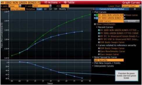
Commenting on the yield spreads of green bonds Bloomberg markets published Figure 2 in 2015 implying that green bonds pay a lower yield than standard bonds. The comparison is made without controlling for any of the variables known to explain yield spreads so the result is questionable.
Figure 2 Green and brown yield spread (Bloomberg Market Specialist, 2015). Bloomberg show that Green bonds pay lower yields than standard ones. The comparison is made without controlling for
17 Song Han and Xing Zhou (2012) study if a larger degree of information asymmetry will lead to a widening of the yield spread. By using microstructural models they estimate the
information asymmetry and then incorporate it into empirical models used to estimate the yield spread of corporate bonds. They conclude that if there is large information asymmetry in the market for a specific corporate bond, the investors will demand a higher yield for holding that bond to compensate them for the information asymmetry.
2.3
Chapter Summary
This chapter starts with a brief overview of basic bond theory, presenting concepts relevant for the essay and models such as duration and yield to maturity. Moving on to previous research, we find that many of the articles and reports about green bonds are uncritically praising the great new asset class and discussing ways to make it grow even faster. A common theme is the call for a certification or verification system. The articles and reports have recently concluded that the green bonds will likely singlehandedly fulfill the goal for private investment set out in the Copenhagen accord in 2009.
In the quantitative part of the previous research we summarize articles about bonds that have in some way impacted our method, models or conclusions. Since none of the articles studies green bonds the results are mainly relevant to help us interpret our empirical results. Our focus is hence mostly on the method and models.
18
3
Methodology
3.1
Research Approach
This is a quantitative study of green bonds, comparing them to similar standard bonds issued by the WB. We focus on changes in price, initial yield to maturity and volatility.
3.2
Data Collection Method
We focus on corporate bonds issued by the WB using bonds that are as similar as possible in all aspects except for being green or not. Swedbank have graciously supplied us with bond data. The data is mid-market data as reported by Bloomberg and Swedbank. In cases where we lack a price, i.e. only have a bid and ask we follow the common practice and construct a midpoint price. We also collect index data from the Federal Reserve Bank of St. Louis and S&P. When the numbers of observations differ between bonds we crop the longer ones to create a balanced dataset, descriptive statistics cover the original datasets.
3.3
Empirical Method
Our main strategy is to insert a green dummy into models, previously applied in other studies, to estimate the price and yield spread of corporate bonds in the articles that have influenced our approach.
19 To compare the volatility of the two types of bond and test hypothesis one, we use roughly the same framework as previous volatility studies (e.g., Blume, et al. 1991; Heinke, 2006). Our data allows us to apply a somewhat more simplistic method since all the bonds have the same issuer, WB. We pool the bonds into two datasets, and create a green and a brown dataset. By running a level regression on the pools with the first difference of the yield spread as the dependent variable we control for anticipated changes in the yield spread. At this point the residuals should represent the unexplained volatility. Lower volatility for the green residuals would support hypothesis one.
To test the YTM at issue we use a method roughly similar to the one used by Lindvall (1977). By running a regression on the initial yield spreads of the WB bonds we test if there is a significant difference in the initial spread between “risk-free” treasuries and the two different classes of bonds. We use a number of control variables to control for changes in the yield spread, risk and what market the bond was issued in. By introducing a green dummy we estimate the effect of being green. Our second hypothesis would be supported if there is a significant negative green effect.
To test for a positive effect on price, we run a regression on the panel-data with a green dummy. Controlling for all factors that may be expected to have an impact on the price and yield changes and with the first difference of the price and yield as the dependent variables. This approach is used in many articles (e.g., Douglas, Huang & Vetzal, 2014; Han & Zhou, 2014; Greenwood & Hanson, 2013; Elton, et al. 2001) and although they do not ask the same questions as in this study, we can apply roughly the same method to test our hypothesis. A significantly positive green effect in the price regression and a negative effect in the yield regression would support hypothesis three.
20
3.4
Data Presentation
3.4.1
Data Used to Test Price Changes and Volatility
To examine the price changes and volatility of green bonds we compare their daily prices and yield to similar brown bonds. For test-results and descriptive statistics see the appendix.
Description
3.4.1.1
To test hypothesis one and three we use a dataset containing panel-data for 2013 and 2014. All our bonds were issued before 2013 and we end the sample before the first bond has less than 365 days left to maturity. The data cover 503 price observations for 22 bonds issued by the WB. It covers all eleven green five-year bonds issued during our sample period and the eleven standard bonds issued at the closest date to the mean time of issue for the greens.
Specifically, excluding the variables that are identical for all bonds, the data contains:
Bid: The end of day bid Ask: The end of day ask Bid-Ask: The bid-ask spread (Ask-Bid)
YTM: The yield to maturity Issue date: The date of issue
Number of trades
Date of maturity: The date of maturity Coupon frequency: How often the bond pays a coupon
Coupon: The coupon rate
TY: The yield to maturity of matched treasuries, issued at roughly the same time as the bond and with roughly the same date of maturity
The eleven green and eleven standard bonds, are all five year bonds issued between late 2009 and early 2012 with the majority being issued during 2010 and 2011. All bonds are dollar denominated.
21 We also have access to matched five year US treasury bonds, i.e. dollar denominated
treasuries issued at roughly the same time as the WB bonds. For all bonds we have five-year treasuries issued within a week of the WB bonds. Using the treasury data we match each WB bond with the appropriate treasury and get a matched treasury yield to maturity (TY) for each date and bond. The yield spread is defined as the yield to maturity of the bond minus the yield to maturity of the matched treasury (for definition see 2.1.5).
The bonds in each class are very similar. Green bonds share very much with the other green bonds and brown bonds with the other brown bonds. This allows us to separate the dataset into one green and one brown part and to create one green and one brown pooled dataset (see appendix for descriptive statistics). We use this to compare the volatility of the two classes.
Characteristics and Calculations
3.4.1.2
Using standard bond theory we calculate the duration, days to maturity (DTM), yield to maturity (YTM) and the yield spread (YSP) of the bonds. We include a dummy; Green, which is one if a bond is green and zero if it is brown.
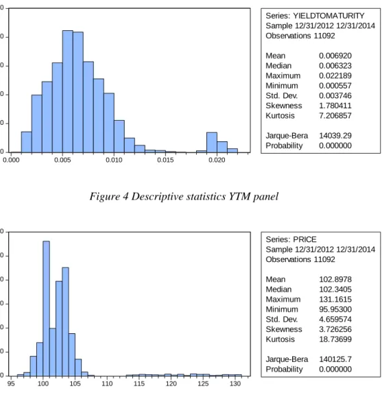
Since we are interested in how being green impact the changes in price and yield to maturity, the main dependent variables in the panel-dataset in this study are Price and YTM (see appendix: Figure 4 and Figure 5). Both are non-stationary; have a unit root and are auto correlated (see appendix: Table 6).
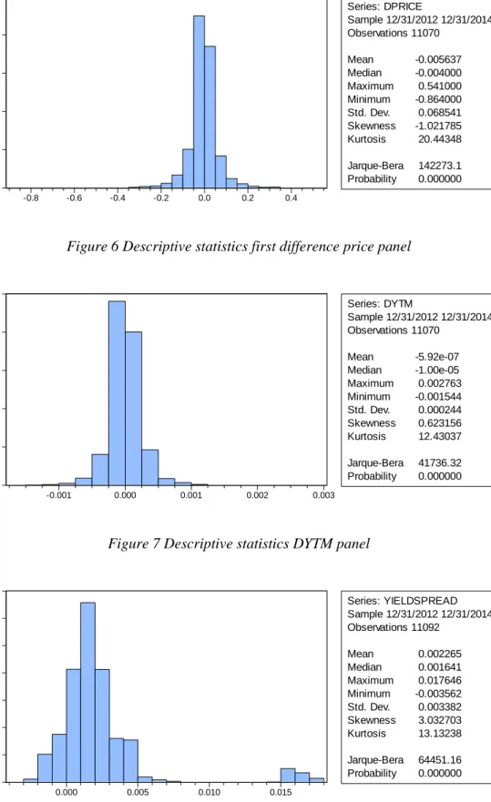
The first difference for Price (DPrice) and the first difference for YTM (DYTM) are both stationary and not auto correlated. An economic interpretation of DPrice is the return from holding the bond for one day, i.e. the daily return. This is not exactly true; the return would have to be normalized by the initial price. But since we are not interested in the exact daily returns, we are comfortable saying that a higher DPrice means a higher daily return for the owner. Since all bonds in the study have fixed coupon size, DYTM can be interpreted as approximately the inverse of the daily return for the owner, for a theoretical framework see chapter two.
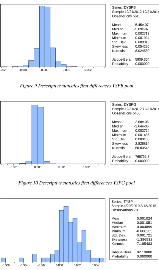
22 Pooling the data for each class generates one green and one brown yield spread (YSPG) and (YSPB). And since they are a subset of the same dataset, the variables above exist in both pools. The YSP variables in the pools have the same characteristics as the YSP variable in the panel-data, i.e. they are non-stationary and auto correlated. To remedy this we use the first difference green yield spread (DYSPG) and first difference brown yield spread (DYSPB), both are stationary and not auto correlated (see appendix).
The control variables; duration, DTM and TY, all have unit roots and are auto correlated in the panel and in the pools. However they are all first difference stationary.
3.4.2
Data Used to Test Initial Yields
To test if the initial yield spread differs between green and brown bonds, we examine the initial yields of all bonds issued by the WB from 2009-2015. We choose the time frame to include all the greens issued by the WB with fixed coupons.
Description
3.4.2.1
The dataset is a time-series covering 96 bonds issued by the WB from 2009-2015. The bonds are all the, fixed coupon, dollar denominated bonds issued in the sample period. After
eliminating outliers, i.e. bonds bundled with derivatives, we are left with 78 observations and a time series starting in 2009 and ending in late 2014 with the variables:
Price: The initial price of the bond in the primary offering, 100 is par YTM: The yield to maturity
Issue date: The date of issue Date of maturity: The date of maturity Coupon frequency: How often the bond pays a coupon
Coupon: The coupon rate
Sub agency issuer: What part of the WB issued the bond (INTL BK RECON & DEVELOP; INTL FINANCE CORP)
Market issued in: Where was the bond issued (DOMESTIC MTN; GLOBAL; EURO MTN) AMM: Amount issued
Senior: A dummy for senior or not (senior =1, Subordinated = 0)
23 The greater heterogeneity in this dataset means that there are a larger number of relevant variables.
Characteristics and Calculations
3.4.2.2
Using standard bond theory we calculate the duration, days to maturity (DTM), yield to maturity at issue (YTM) and the yield spread (TYSP) of the bonds. Also a dummy variable; Green, that is one if a bond is green and zero if it is brown, is added.
Our main dependent variable in the time series is YTM, to make this variable stationary i.e. take away the trend, we calculate the yield spreads. The time series yield spread, TYSP, is stationary and auto correlated (see appendix).
To correct for changes in the yield spread between AAA corporate bonds and the “risk-free” treasuries we introduce the S&P U.S. Issued AAA Investment Grade Corporate Bond Index 5yr (S&P Dow Jones Indices LLC, 2015).
The variables that end up being part of the finished model after paring down (see 4.2.1) are S&P U.S. Issued AAA Investment Grade Corporate Bond Index (S&P), Green, Duration, Global, Domestic (Dummies for market, leaving out Euro), Amm.
3.4.3
Testing for Unit Roots in the Data
When performing a unit root test on our panel-data we mainly rely on the test set out by Levin, Lin & Chu (2002). To explore robustness, we also apply two other specifications, the test specified by Im, Pesaran & Shin (2003) and the ADF – Fisher test. We use both EViews and Matlab to perform these tests and present the results in the appendix. In two cases the tests differ in their results, indicating a common unit root but not individual unit root processes. In these cases we apply the unit root test specified by Hadri & Larsson (2005), where stationary is the null hypothesis and we strongly reject the null for both variables.
24 In the time series case we use the Augmented Dickey-Fuller test as specified by Verbeek (2012a) to test the TYSP for a unit root. The variable is stationary and somewhat auto correlated (see appendix Table 8).
3.5
Validity and Reliability
Receiving data from Swedbank have been absolutely essential for this study, but it means that we have not been personally involved in the majority of the data collection. There is no reason to suspect that the data received from Swedbank is in any way altered or differ from the original data in the Bloomberg database; we find it highly unlikely that this would be the case, but we cannot guarantee that the data is not altered knowingly or by mistake.
The WB issues all the bonds in our dataset, except for the treasuries. Thus the results are not immediately generalizable to green bonds issued by any borrower. We find it plausible however that the results are at least generalizable to other AAA bonds, and that future “certified” bonds will behave roughly like the ones in our dataset.
The comparatively few bonds in our panel-dataset mean that we have relatively few cross-sections. This is potentially a problem as the data is very non-normally distributed for most variables and most tests assume normal distributions for small/finite sample consistency. This is also a potential problem when running the regressions since the comparatively few cross-sections and non-normal distribution may result in erroneous results. We have tried to remedy this as far as possible, taking insights from relevant articles (e.g., Costantini et al. 2015; Westerlund & Basher 2008; Westerlund 2014; Im, et al., 2014) into account. When the results have been ambivalent or inconclusive, we have tried to find more robust ways to test our conclusions.
25
3.6
Chapter Summary
This chapter presents the method and the two datasets (one for brown, one for green bonds) used in our study. Our strategy is to insert our green variable into models describing the yield spread and price of corporate bonds.
The data accounts have a descriptive part and a part focusing on important characteristics. All the main variables turn out to be trend and difference stationary. To eliminate the trend we calculate the yield spread; the difference between the bonds in our study and matched treasuries. The yield spread is stationary in the time series but not in the panel-data.
In the end of the chapter we discuss possible problems stemming from the data, we conclude that the relatively few bonds in our panel is the main problem aside from the homogeneity of the sample. These problems do however turn out to be manageable.
26
4
Empirical Analysis and Discussion
4.1
Testing Volatility
To be able to compare the unexplained volatility of the two types of bond we estimate a pooled feasible generalized least squares (FGLS) model (Verbeek, 2012b) with the yield spread as a dependent variable and compare the volatility of the residuals.
Specifically our strategy is to use existing models, developed to explain changes in the yield spread (e.g., Campbell & Taksler, 2003; Han & Zhou, 2013) and estimate the model for each pooled dataset. The models are based on a structural view of corporate default. In this type of model the firms’ credit risks depend on its capital structure and a number of observable macro variables. In some cases we use different proxies for a bond’s credit risk, but we try to adhere to the models when possible. Since all bonds in our study are issued by the WB, they all share the same issuer specific characteristics. Because of that, bond-specific characteristics such as duration and liquidity are the main variables explaining the differences in yield and price between the bonds. Consistent with the literature, we propose that differences in YTM and Price between the WB bonds should be a function of; Treasury yields, liquidity, Coupon, DTM, Coupon frequency and idiosyncratic risks that apply to the particular bond (see 2.1)
27
4.1.1
Testing for Model Specification
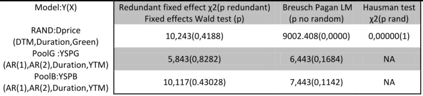
To decide which model will be the most appropriate for this part of the study we test for specification following the framework set out by Baltagi (2005) and start by estimating our raw model with fixed effects and perform a redundant fixed effect test. Since the null is true, i.e. the fixed effects are redundant, we move on to performing a Breusch & Pagan Lagrange multiplier (LM) test (Breusch & Pagan, 1980) and a Hausman test (Baltagi, 2005). We run all tests both in EViews and Matlab except the LM test, which we only perform in Matlab since it is hard to do in EViews. For results see appendix.
The outcome of the tests show that a pooled feasible generalized least squares (FGLS) model is the appropriate (Baltagi, 2005).
4.1.2
Model Specification and Estimation Methods
We find that we can use a much simpler model than the ones used in the articles inspiring our model. After testing that it does not impact the results, we use duration to represent the effect of coupon size and frequency as suggested by multiple authors (2.2.2). We start with roughly the same model as the one employed in Han & Zhou (2013) and pare down. To pare down we use the F-statistic, the Akaike information criterion and the Log likelihood ratio to control for the significance of the loss of information from removing a variable (Vuong, 1989; Arnold, 2010). When the methods agree with each other we eliminate a variable. We end up with regression one:
28 D indicates first difference. We use Bid-Ask as a proxy for liquidity as recommended by Longstaff, et al. (2005). As an outcome of the tests we run regression one using pooled feasible GLS as specified in Pedroni (2004) with no random or fixed effects. We do this twice, once for each of the pools. We then make a straight up comparison of the volatility of the residuals using a Wald-test and a Brown-Forsythe test as specified by Brown & Forsythe (1974).
4.1.3
Empirical Results
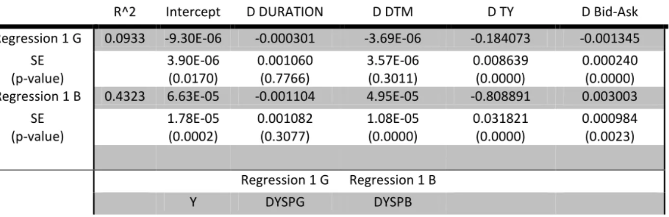
To control for expected changes in the yield spread we run regression one for both datasets (Table 1), and compare the volatility of the residuals. The estimated parameters are very different between the pools. This is in itself a strong sign that the two types of bond behave differently. To present consistent estimations of the parameters, we show the results estimated with cross-section SUR corrected residuals. We present the results with the corrected
residuals in Table 1 to give the reader the consistent estimates. The residuals that are presented in Figure 3 and compared in Table 3 are uncorrected.
Table 1 Results from running regression one on the green and brown pool: Controlling for expected volatility. The regression use variables that are known to explain changes in the yield spread of
corporate bonds. Note the very different estimation of the parameters for the two pools.
R^2 Intercept D DURATION D DTM D TY D Bid-Ask Regression 1 G 0.0933 -9.30E-06 -0.000301 -3.69E-06 -0.184073 -0.001345
SE (p-value) 3.90E-06 (0.0170) 0.001060 (0.7766) 3.57E-06 (0.3011) 0.008639 (0.0000) 0.000240 (0.0000) Regression 1 B 0.4323 6.63E-05 -0.001104 4.95E-05 -0.808891 0.003003
SE (p-value) 1.78E-05 (0.0002) 0.001082 (0.3077) 1.08E-05 (0.0000) 0.031821 (0.0000) 0.000984 (0.0023) Regression 1 G Regression 1 B Y DYSPG DYSPB
29 It is interesting to note the difference in R2 (0.093302 compared to 0.432375), the difference stems from the relatively low correlation between the green bonds and the control variables. Running the regression with lagged D TY (see appendix Table 5) shows that both the first and second lag are significant for the green bonds while all lags are highly insignificant for the brown dataset. A regression identical to regression one but with the two significant lags of D TY raise the R2 to approximately 13% for the green dataset. The fact that the lagged treasury yield is so significant supports the hypothesis that the green investors are reacting slowly to changes in the macro environment.
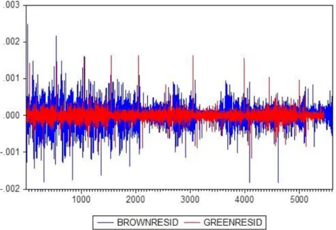
The main purpose of running regression one was to estimate the unexpected volatility of the green- and brown bonds respectively. When comparing the residuals after the two regressions, the difference is immediately noticeable just by looking at the two sets of residuals in
Figure 3:
Figure 3 Brown and green residuals generated with original datasets and without correcting for heteroscedasticity
The residuals are not auto correlated but heteroscedastic; this is corrected in the estimations presented in Table 1. As evident from Figure 3 the brown residuals are much more volatile than the green ones.
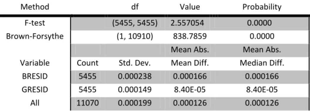
30 The tests indicate a significant difference in volatility between the two datasets (Table 1).
Table 2 Volatility comparison between brown and green residuals after regression one. Note that the volatility of the two pools are significantly different, and that the green pool exhibits much lower
volatility.
Method df Value Probability F-test (5455, 5455) 2.557054 0.0000 Brown-Forsythe (1, 10910) 838.7859 0.0000
Mean Abs. Mean Abs. Variable Count Std. Dev. Mean Diff. Median Diff.
BRESID 5455 0.000238 0.000166 0.000166 GRESID 5455 0.000149 8.40E-05 8.40E-05 All 11070 0.000199 0.000126 0.000126
The green bonds are roughly a third as volatile (σ2
B = 0.00000005664 and σ2G= 0.00000002220) as the standard bonds.
4.2
Testing Initial Yield Spreads
To quantify the effects of being green on initial yield spreads i.e. testing hypothesis two, we run a time series regression on initial yield spreads between the bonds issued by the WB and the matched treasuries. We use the same strategy as above i.e. use existing models developed to explain changes in the yield spread (e.g., Campbell & Taksler, 2003; Han & Zhou, 2013) but in this case we insert a green dummy into the model and thereby estimate the effect of being green. We basically use the same proxies and variables as in 4.1.
31
4.2.1
Model Specification and Estimation Methods
We insert our green dummy into an existing model used in previous research to explain differences in the yield spread. Thus we start out with a large model containing as many of the variables that have been found to impact the yield spread of corporate bonds as we can find data or reasonable proxies for. Specifically we use all variables in the dataset (3.4.2.1) and proxies for corporate yield spread and liquidity. Following the models that inspire our method we also use Swap and CDS data, taken from DataStream (Thomson Reuters, 2015). Since the CDS and Swap are dropped in the paring down process, and does not make it into any of our models we do not describe this data further. Results are available upon request. We then par down using the same method as above (see 4.1.2). Since the TYSP variable is auto correlated we use an AR (2) model, regression two:
4.2.2
Testing the Model
We use a Chow forecast test (Chow, 1960)) to test the stability of the estimated relation over the sample period. Further we apply a Ramsey RESET Test as specified in Papke &
Wooldridge (1996) to test for miss-specification and a Jarque–Bera test (Jarque & Bera, 1987) to test the residuals for normality. To test the residuals for heteroscedasticity we use the Breuch-Pagan-Godfrey LM-test (Verbeek 2012b; Breusch & Pagan 1980) and since the results are a borderline pass, we run the regression with White heteroscedasticity-consistent standard errors (Verbeek, 2012b). Finally we run a Breusch-Godfrey Serial Correlation LM Test (Breusch & Pagan, 1980), the model pass all the tests with flying colors, for test statistics see appendix.
32
4.2.3
Empirical Results
The main result presented in Table 3, is the sign of the green parameter. We estimate the effect of being green in the initial yield to 0.000944; it is a statistically significant result.
Table 3 Results from running regression two: Estimations of variables effect on initial yield spread. The green parameter is positive and significant.
Variable Coefficient Std. Error t-Statistic Prob. S&P 0.062147 0.032381 1.919270 0.0592 GREEN 0.000944 0.000467 2.020685 0.0473 DURATION -0.000224 9.24E-05 -2.420491 0.0182 GLOBAL 0.001076 0.000402 2.676880 0.0093 DOMESTIC_MTN 0.001606 0.000414 3.877829 0.0002 AMM 1.69E-07 1.40E-07 1.207614 0.2314 Intercept 0.000556 0.000334 1.664949 0.1006 AR(1) -0.259287 0.122148 -2.122732 0.0375 AR(2) 0.113700 0.122297 0.929705 0.3559 Adjusted R2 0.466469
We find that green bonds have paid a higher yield than the standard bonds. The green effect is larger than that of the amount issued and roughly the same as that caused by being issued in different markets.
4.3
Testing Price and Yield Changes: Specification
In this part of the chapter we use the same variables and proxies as in 4.1. and also we make the same assumptions. This time we insert the green dummy straight into existing models used to explain changes in the yield spreads (e.g., Campbell & Taksler, 2003; Han & Zhou, 2013). We also apply the same procedure to test for the appropriate model specification as in 4.1.1.
33 For this estimation we use the full panel dataset i.e. we do not divide it into green and brown parts. After testing for specification we use an estimated generalized least squares model (EGLS) with random effects as detailed in Baltagi (2005).
4.3.1
Model Specification and Estimation Methods
By using the same method as in 4.1.2. to par down the original much larger model we get regression three and four :
D indicates first difference. We use Bid-Ask as a proxy for liquidity as recommended by Longstaff, et al. (2005). However the liquidity proxy does not make it into the final model. The result of testing for model specification is that we use an estimated generalized least squares model (EGLS) as detailed in Baltagi (2005) with random cross section effects. We estimate regression three and four in EViews and Matlab using cross section random effects, Swamy-Arora weighting as specified in Baltagi (2005) with EGLS and Cross-section SUR corrected residuals to ensure against heteroscedasticity.
34
4.3.2
Empirical Results
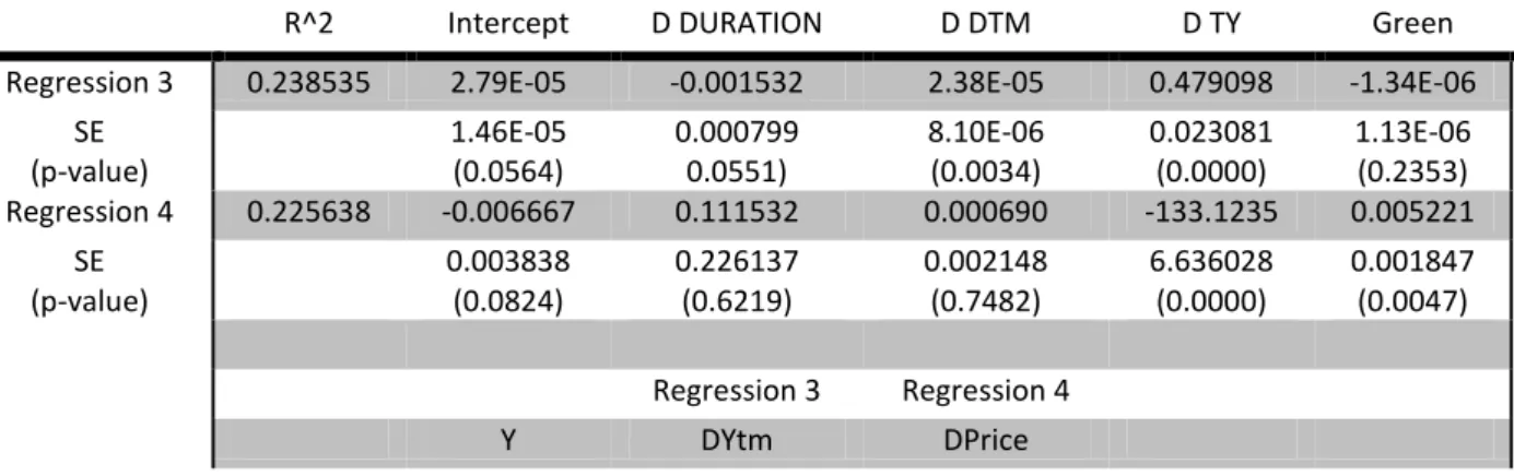
In Table 4 we present the estimated parameters from running regression three and four as specified above. The purpose of the estimations is to test the effect of being green on the first differences of yield and price.
Table 4 Results from running regression three and four: Estimations of variables effect on first differences of yield and price. Note the estimation of the green parameters
R^2 Intercept D DURATION D DTM D TY Green Regression 3 0.238535 2.79E-05 -0.001532 2.38E-05 0.479098 -1.34E-06
SE (p-value) 1.46E-05 (0.0564) 0.000799 0.0551) 8.10E-06 (0.0034) 0.023081 (0.0000) 1.13E-06 (0.2353) Regression 4 0.225638 -0.006667 0.111532 0.000690 -133.1235 0.005221 SE (p-value) 0.003838 (0.0824) 0.226137 (0.6219) 0.002148 (0.7482) 6.636028 (0.0000) 0.001847 (0.0047) Regression 3 Regression 4 Y DYtm DPrice
If the results are to be consistent with previous studies the coefficients of the control variables would be expected to carry opposite signs. This is generally what we see in Table 4. The results from the yield regression is mainly noticeable for the lack of significance of the green dummy parameter (β4). We do however note that the sign of β4 is negative. Regression two on the other hand has a clearly significant; quite large, positive green dummy parameter (β4).
35
4.4
Robustness of Results
We have tried to double check our results when appropriate. In most cases we have used both EViews and Matlab to estimate our regressions. To ensure robustness we have used
alternative specifications for all our models, running the ones in the articles used for inspiration and other variations suggested by the literature (e.g., Baltagi, 2005; Verbeek, 2012b). The alternative specifications support our results, and confirm that we use the right models. As an example of this we have run all the panel data regressions with fixed effects as recommended by Baltagi (2005). We do this to make sure that the parameters are estimated approximately the same; naturally with different standard errors, and this test turn out to validate our models in all cases.
To ensure that the results in the third hypothesis are not a product of the daily data, we run the model on the weekly changes i.e. using first differences of weekly price and yield instead of daily. The results are in line with those in Table 4 but not significant. Results are available upon request.
The estimation of the green effect on the initial yield spread turn out to be very robust to different model specifications; the estimated parameter is roughly the same in all of our control regressions. The parameter is almost identically estimated in the initial pre paring down model. It is worth mentioning that about half of the green bonds were issued during 2010 and 2011, this is the period when there was a pullback in the yearly amount issued (Figure 1). We speculate that this might be one of the main factors behind the estimated green effect on the initial yield spread. Results are available upon request.
36
4.5
Discussion
4.5.1
Hypothesis One
To test hypothesis one, we compare the unexpected volatility of the two different bond types. The green bonds are approximately a third as volatile as the standard ones. Our tests confirm that there is a significant difference in volatility. We take this as a confirmation that the green bonds have been much less volatile during our sample period and as strong support for hypothesis one.
We believe that there are three main reasons behind the results. Firstly one should look at the type of investors whom according to the articles and reports referenced in chapter 2 were most likely to invest in green bonds, especially in the early part of the sample period. The typical investor was probably forced into green investing either by policy or public pressure
(Mathews & Kidney, 2010). This kind of investor is in our view rather unlikely to sell their green bonds in a downturn since there are no obvious alternative investments. Moreover such an investor is probably less likely to mark its assets to market (Coats, 2008).
The second reason might actually be found in our refutation of hypothesis two. We find that investors were paid a yield premium to invest in green bonds. An investor who bought a green bond in for example 2010 and now earn a higher yield from that bond compared to a similar standard bond; bought at the same time (see 4.2.3) is likely to have a hard time finding an investment that offer the same risk-reward. This could mean that the investor have an extra incentive to hold on to the higher yielding green bond.
37 Thirdly as the number of investors wishing to invest in green bonds grew, it is likely that supply did not keep up (Grene, 2015). This could explain the low correlation between the green dataset and the control variables (see Table 1). Investors buying green bonds in this demand driven market will be less likely to quickly divest or let the normal risk measures dictate what yield is acceptable (Clapp, 2014). Hence the impact of exogenous events will have less or a lagged effect on the green yield. Actually our results show that the green bonds correlate heavily with lagged treasury yields and very little with any of our other control variables.
4.5.2
Hypothesis Two
To test our second hypothesis we compared the initial yields of 78 bonds issued by the WB. As Table 3 show the results lead us to reject our hypothesis. It is clearly the case that, contrary to our previous assumptions, the yield at issue is higher for the green bonds then for the similar standard ones during the sample period.
Many of the green bonds in the data are issued during 2010 and 2011. By looking at Figure 1: Growth of green bond market it is obvious that during 2010 a much larger amount of green bonds was issued than in the years before and after. It seems that the rapid increase of the amount issued outpaced the demand as very few investors knew, or was comfortable with the new asset class. The subsequent shrinking of the amount issued (Figure 1) and the calls for governments to support the asset class, provide backing to this explanation (Mathews & Kidney, 2010).
38 Han & Zhou (2013) point to another possible explanation. The information asymmetry;
traders unfamiliar with green bonds may avoid them or demand high premiums to buy the bonds. When traders/investors are not comfortable with an asset class, it likely does not matter how similar the bonds are to standard ones. Even with exactly the same credit risk the investors may still avoid them. Green bonds are not significantly less liquid than brown ones; at least if one accepts Bid-Ask as a proxy for liquidity, using roughly the same testing
methodology as in 4.1 we do not find a significant difference. All the same we find it likely that a market with few well informed investors and many new or ill-informed actors will show the effects described by Han & Zhou.
4.5.3
Hypothesis Three
To test hypothesis three we estimate the effect of being green on the first difference of price and yield. The green effect is significant and positive in the case of price, and negative but not significant for the yield. We view the results as support for hypothesis three. The green bonds have evidently had a stronger price development during the sample period and even though the yield parameter is not significant, bond theory dictates that the opposite must be true for yields (La Grandville, 2001).
We propose that the evolution of the market for green bonds is the main reason behind these results. The market is still in its infancy but in 2010 and 2011 when the bonds in this study were issued the asset class was new and unknown (Mathews & Kidney, 2010). As green bonds have become better known to traders and investors, they have been upgraded in the eyes of the market. No longer seen as a new and probably risky asset class, the bonds are now an accepted and for many investors essential investment vehicle (Bloomberg Finance, 2014). The initial yield premium demanded by investors; evident in out testing of initial yields, have likely been erased and is probably replaced by a discount (Bloomberg Market Specialist, 2015).
39 The growing demand apparent in the explosive growth of the market with new mutual funds, investable indexes and reports of large investors buying massive amounts of green bonds is a sign that demand may well outstrip supply. Blackrock (BlackRock Inc., 2015) alone have made it known that they will invest two billion dollars in green bonds during 2015, meaning they would buy more than half of all bonds issued just three years ago (Bloomberg Finance, 2014; Grene, 2015).
The catch-up effect probably explains part of the difference between the green and standard bonds. But we consider the estimated green effect (Table 4) to be rather large. It is certainly larger than what we would expect from the catch-up mechanism alone. The yield penalty estimated in 4.2 is compensated in a time much shorter than our sample period, and we interpret the results as support for hypothesis three.
4.6
Chapter Summary
In the first part of the chapter we find support for hypothesis one and we see no results that makes us doubt that the volatility of the green bonds is lower than that of the brown ones. We expect the lower volatility to persist into the near future.
In the second part we reject our second hypothesis because our results show that green bonds have paid higher initial yields than the standard bonds, during our sample period. Most likely the newness of the green bonds and the resulting information asymmetry is part of the
explanation. We do not expect this to persist.
In the last part of the chapter we find support for our thirds hypothesis. We find that the green bonds have significantly positive price development compared to s