Supervised classification with conditional
Gaussian networks: Increasing the
structure complexity from naive Bayes
Aritz Pe´rez
*, Pedro Larran˜aga, In˜aki Inza
Intelligent Systems Group, Department of Computer Science and Artificial Intelligence, University of The Basque Country, P.O. Box 649, Donostia 20080, San Sebastian, Spain Received 22 February 2005; received in revised form 11 August 2005; accepted 16 January 2006
Available online 13 February 2006
Abstract
Most of the Bayesian network-based classifiers are usually only able to handle discrete variables. However, most real-world domains involve continuous variables. A common practice to deal with continuous variables is to discretize them, with a subsequent loss of information. This work shows how discrete classifier induction algorithms can be adapted to the conditional Gaussian network par-adigm to deal with continuous variables without discretizing them. In addition, three novel classifier induction algorithms and two new propositions about mutual information are introduced. The clas-sifier induction algorithms presented are ordered and grouped according to their structural complex-ity: naive Bayes, tree augmented naive Bayes, k-dependence Bayesian classifiers and semi naive Bayes. All the classifier induction algorithms are empirically evaluated using predictive accuracy, and they are compared to linear discriminant analysis, as a continuous classic statistical benchmark classifier. Besides, the accuracies for a set of state-of-the-art classifiers are included in order to justify the use of linear discriminant analysis as the benchmark algorithm. In order to understand the behavior of the conditional Gaussian network-based classifiers better, the results include bias-vari-ance decomposition of the expected misclassification rate. The study suggests that semi naive Bayes structure based classifiers and, especially, the novelwrapper condensed semi naive Bayes backward, outperform the behavior of the rest of the presented classifiers. They also obtain quite competitive results compared to the state-of-the-art algorithms included.
2006 Elsevier Inc. All rights reserved.
0888-613X/$ - see front matter 2006 Elsevier Inc. All rights reserved. doi:10.1016/j.ijar.2006.01.002
* Corresponding author.
E-mail addresses:[email protected](A. Pe´rez),[email protected](P. Larran˜aga),[email protected](I. Inza). 43 (2006) 1–25
Keywords:Conditional Gaussian network; Bayesian network; Naive Bayes; Tree augmented naive Bayes; k-Dependence Bayesian classifiers; Semi naive Bayes; Filter; Wrapper
1. Introduction
Supervised classification is a basic task in data analysis and pattern recognition. It requires the construction of a classifier, that is, a function that assigns a class label to instances described by a set of variables. There are numerous classifier paradigms, among
which Bayesian networks (BN) [48,50], based on probabilistic graphical models (PGMs)
[3,42], are very effective and well-known in domains with uncertainty. A Bayesian network is a directed acyclic graph of nodes representing variables and arcs representing condi-tional (in)dependence relations between the variables. This kind of PGM assumes that each random variable follows a conditional probability function given a specific value of its parents.
Usually the conditional probability function is assumed to be multinomial [3,48,50].
This kind of BN is known as aBayesian multinomial network(BMN)[3]. It handles
dis-crete variables only and, thus, if a continuous variable is present, it must be discretized,
with a subsequent loss of information[63]. A battery of BMN-based classifier induction
algorithms has been proposed in the literature: naive Bayes [11,39,46], tree augmented
Bayesian network[17],k-dependence Bayesian classifier[57]and semi naive Bayes[37,49].
In the presence of continuous variables, another alternative is to assume that continu-ous variables are sampled from a Gaussian distribution. This kind of Bayesian network is
known as aconditional Gaussian network(CGN)[2,19,42–44]. It can deal with discrete and
continuous variables and, therefore, it is an alternative to work with mixed variables with-out the need to discretize the continuous ones. A structural constraint of the CGN is that a discrete variable cannot have continuous parents. Although the Gaussian assumption for continuous variables is very strong, it usually provides a reasonable approximation to
many real-world distributions [30]. The classifiers, inducted by the algorithms presented
in this paper, are restricted to CGN models with continuous predictor variables and discrete class variable, which is the parent of all predictors included in the model. The structures of these classifiers range the simplest naive Bayes structure to the complete graphs.
A classifier based on BNs can be constructed from aBayesianapproach[2,19,22,27]. It
takes into account all possible models and all possible parameters, restricted to a special kind of structure and a family of probability functions. However, the classifiers included in this paper are induced from a non-Bayesian point of view, which fixes a unique structure
and its parameters. The structure is learned guided by a score function (likelihood[24],
accuracy [33,40,49] or mutual information [17,57]). There are a lot of works in which
the non-Bayesian approach for discrete variables is performed with different structure
complexities[11,17,33,37,39,40,46,49,57]. The non-Bayesian approach, to learn classifiers
based on conditional Gaussian networks, is performed for mixed variables in the work of
Friedman et al.[18].
BN-based classifiers can be inducted in two ways depending on the distribution to be
of the joint probability function of the predictor variables and the class. They classify a new instance by using the Bayes rule to compute the posterior probability of the class var-iable given the values for the predictors. On the other hand, discriminative classifiers
[24,58] directly model the posterior probability of the class conditioned to the predictor
variables. The learning can also be done in a mixed way, as shown in [55]. The present
work is performed from the point of view of generative learning.
This paper presents the CGN paradigm and a battery of classifier induction algorithms supported by it, much of them adapted from the previous enumerated algorithms sup-ported by the Bayesian multinomial network paradigm. Besides, two new propositions about mutual information, necessary to design filter approaches, are introduced. The clas-sifier induction algorithms presented are experimentally compared by means of estimated
predictive accuracy. The bias-variance decomposition[36]of the expected misclassification
cost is performed in order to analyze the behavior of the CGN-based classifiers presented in more detail.
The paper is organized as follows. In Section 2, four kinds of well-known classifier
structures are introduced: naive Bayes, tree augmented naive Bayes,k-dependence
Bayes-ian classifier, and semi naive Bayes. Based on each kind of structure, different classifier induction algorithms to handle continuous variables are presented. Three of the presented
algorithms are novel algorithms: the filter selective ranking naive Bayes, the wrapper
k-dependence Bayesian classifier, and the wrapper condensed semi naive Bayes. Moreover,
seven algorithms are adapted from the Bayesian network paradigm to the CGN one. In the same section, a classifier induction algorithm taxonomy is proposed, based on wrapper
and filter concepts. In Section3, experimental results in classification tasks and their
bias-variance decompositions in each data set are shown for CGN-based and benchmark
clas-sifiers. Finally, in Section4, our conclusions and future work are presented.
2. Adapting Bayesianmultinomialnetwork-based classifier induction algorithms to continuous domains
PGMs are used to encode the joint distribution among the domain variables, based on the conditional independencies represented by the graph structure. This fact, combined with the Bayes rule, can be used for classification. In order to induce a classifier from data,
we consider two types of variables: the class variable or classC, and the rest of variables or
predictors, X= (X1,. . .,Xn). This paper only considers PGMs whose class variableCis
the root of the graph. In other words, {C}Pai(i= 1,. . .,n) wherePaiis the set of
vari-ables that are parents of Xi in the graph. The process of classifying an instance
x= (x1,. . .,xn) consists of selecting the class with the highest a posteriori probability,
P(cjx). This entails the use of the winner-takes-all rule[11]. This rule is used when the loss
function value, which gives a measure of the cost of misclassification, is symmetric. The classification process can be done in the following way with CGN:
PðcjxÞ /pðc;xÞ ¼PðcÞpðxjcÞ ¼PðcÞY
n
i¼1
pðxijpaiÞ ð1Þ
wherepaidenotes a value ofPai. Moreover,[3,8,19]
wheremijcandvijcare defined as follows[19]: mijc¼lijcþX ni j¼1 bijjcðxjljjcÞ ð3Þ vijc ¼jRXi;PXijcj jRPXi jcj ð4Þ
PXiis the set of continuous predictors that are parents ofXi, soPXi=Pain{C}, andniis
its cardinality.RSjcis the covariance matrix of the set of variables S conditioned to the
class value C=c. rijjc is the covariance between the variables Xiand Xj conditioned to
c, and r2
ijc is the variance of Xi conditioned to c. bijjc is the regression coefficient of Xi
onXjconditioned to the class valueC=c, and is defined as[8]
bijjc¼rijjc
r2
jjc
ð5Þ
The process of induction for a classifier supported by the PGMs can be divided into
three main parts:preprocessing,structural learningandparametric learning.
An important issue of thepreprocessingtask consists in transforming the variable space
or selecting the relevant variables which will take part in the classifier induction process. Variable selection and transformation (reducing the number of features) gives some advantages in a classifier induction process: reduction of the search space, easy explana-tion capacity, improvement of the classificaexplana-tion accuracy, and enhancement of the reliabil-ity of its estimation. The transformation of the space of variables tries to construct a set of new artificial variables which usually are mutually independent and capture much of the information of the original space. Standard transformation of the space of variables
includes principal component analysis[32].
The variable selection techniques (see[25]) can be divided into two groups depending on
the nature of the search score used by the selection process: filter [45] and wrapper
approaches[35]. The scores used in the filter approaches are based on intrinsic
character-istics of the data[45]. The advantages of filter approaches are related to the time
complex-ity needed to make the selection. For example, a score based on information theory [6]
used to select variables in a filter manner (entropy and mutual information measures),
iscorrelation based feature selection(CFS)[26,64]. More examples based on information
theory are the approaches based on relevance concepts[60,61]. On the other hand,
wrap-per approaches use an estimated classification goodness measure as a score[35]. Thus, they
depend on the specific classifier used to estimate the classification goodness.
Variable selection is usually considered a preprocessing step, but it can also be consid-ered a part of the structural learning process because the use of different feature subsets
inevitably imposes different models [13]. Besides, sometimes the selection could be
per-formed parallelly to the structural learning process (especially in the wrapper approaches). The search process depends on the score and search strategy used. For a review of different
search strategies, see[38]. Although some of the methods proposed in this work perform
an implicit selection of variables, it is not our purpose to treat this process of selection explicitly.
Structural learningusually involves a search process led by a score value in the space of
possible graph structures. The search process tries to optimize the score. It generally fin-ishes when a local optimum is found. We consider that, structural learning can be carried out in a filter or a wrapper way, depending on the score which guides the search process.
These filter and wrapper concepts are adapted from the feature subset selection literature. In our work, the filter approaches use the mutual information as a score and the wrapper approaches use the estimated predictive accuracy.
The structural learning is constrained by a search space usually defined by means of the kind of (in)dependency and dependencies allowed among the variables or structure com-plexities. Depending on the search space, the algorithms explore, for example, naive Bayes
like structures [11,39,46], tree augmented networks [17,33], k-dependence networks [57],
semi naive Bayes[37,49], unrestricted networks[4,51], or Bayesian multinets[20].
Parametric learningconsists in estimating parameters from the data. These parameters
model the dependence relations between variables, represented by the classifier structure. One of the main advantages of CGNs with respect to BMNs is related to the number of parameters needed to model a continuous domain. In contrast to the exponential number
of parameters necessary to learn a complete graph in BMNs (OðrQni¼1riÞ,1whereriandr
are the cardinality of the variablesXiandCrespectively), the number of parameters
nec-essary to model a complete graph based on CGNs with continuous variables has a low
polynomial rate[19],Oðn2rÞ. Due to the fewer number of parameters, the CGN-based
clas-sifiers tend to has less sensitivity to the changes in the training set. They also adjust the training data sets less than BMN-based classifiers. Therefore, in general, they should have a lower variance and higher bias components in their associated decomposition of the
expected misclassification rate [16,36]. Besides, a lower number of parameters allows a
more reliable and robust computation of the necessary statistics.
Moreover, the parameters can be computed a priori, without taking into account the structure to be considered. More specifically, the necessary parameters are an array of
class conditional covariance matrices,R= (R1,. . .,Rr), and another array of class
condi-tional mean vectorsl= (l1,. . .,lr). The possibility of computing the parameters a priori
allows a more efficient backward structure search compared to BMN-based algorithms. BMNs only handle discrete variables. The continuous variables must be discretized in
order to handle them. There is a loss of information in this discretization process[63]. The
same classifier induction algorithm obtains different classifiers and different classification scores depending on the criteria used to discretize the data. It can be concluded that the lost information depends on the discretization criteria used. On the other hand, CGNs are only able to handle continuous variables assuming that they follow a Gaussian distri-bution. Therefore, information is used erroneously if the real distribution of the variables
defers much from the Gaussian distribution and, thus, the estimation ofp(c,x) tends to
have higher bias term in the estimated error decomposition. However, if the real distribu-tion does not defer much from the Gaussian distribudistribu-tion, the estimated scores of classifiers
based on BMNs and CGNs obtain comparable results (see Section 3). In addition, the
assumption of normally distributed data can avoid the overfit problem when the structure of the graph is too complex, and also tends to obtain an estimation of the joint distribution
with lessvariancedue to the low polynomial rate of parameter.
The following subsections present classifier induction algorithms supported by different CGN paradigms ordered by their structural complexity. The structural complexity is related to the type and number of dependencies allowed between variables. Four types
1
In this work,OðÞ expressions denote complexity orders, sometimes in terms of time (or operations) and sometimes in terms of number of parameters.
of structures are presented:naive Bayes, tree augmented Bayesian network,k-dependence
Bayesian classifierandsemi naive Bayes.
The least complex structure is thenaive Bayes structure(NB structure), which assumes
that predictor variables are conditionally independent given the class. It is not mandatory
to include the entire set of predictor variables. The space of possible NB structure isOð2nÞ.
Thetree augmented Bayesian network structures(TAN structures) break with the strong
independence assumption made by NB structures, allowing probabilistic dependencies among predictors. The TAN structures consist of graphs with arcs from the class variable only to a subset of selected predictors, and with arcs between predictors taking into account that the maximum number of parents of a variable is one plus class.
Thek-dependence Bayesian classifier structure(kDB structure) extends TAN structures
allowing a maximum of k predictor parents plus the class for each predictor variable
(TAN structures are equivalent tokDB structures withk= 1).
Finally, thesemi naive Bayes structure(Semi structure) introducesjoint nodes, which are
the Cartesian product of a subset of original variables. Therefore, every component vari-able of the joint nodes are mutually statistically dependent.
We say that a structure is complete when all variables are included and no more
depen-dencies can be allowed. If not, the structure is incomplete. A completekDBstructure and
an incomplete one withk= 2 are shown inFig. 2.
The structures themselves represent domain knowledge and can be interpreted in terms of conditional (in)dependencies, constructing the associated independence graph. In addi-tion, they can be understood, from the point of view of the classification task, as
simpli-fications of the real joint distributionp(c,x). These simplifications are again based on the
relations of conditional dependency that are inferred from the structure, and they can be represented by means of factorization. This factorization requires fewer parameters than the joint distribution over all the variables.
In the next subsections, for each kind of structure previously introduced, a set of wrap-per and filter classifier induction algorithms are presented.
2.1. Naive Bayes
Thenaive Bayesclassifier (NB)[11,39,46] is characterized by the conditional
indepen-dence assumption between variables given the class. Moreover, all variables are included
in the model, so the classifier structure is given a priori:complete NB structure. The
accu-racy obtained with this classifier in its discrete version is surprisingly high in some domains, even in data sets that do not obey the strong conditional independence
assump-tion[10]. C X1 X2 X3 X4 (a) C X1 X2 X3 X4 (b) C X1 X2 X3 X4 (c) C X1 (X2,X3) X4 (d)
Thanks to the conditional independence assumption, the factorization of the joint
prob-ability is greatly simplified. A NB classifier structure example is shown inFig. 1(a), where
each variable is a class-conditioned independent variable. After adapting Eq. (1) to NB
structure particularities, the following factorization is obtained:
PðcjxÞ /PðcÞY
n
i¼1
pðxijcÞ ð6Þ
with pðxijcÞ Nðlci;rciÞ to model continuous variables conditioned to the class. For
example, the factorization of Fig. 1(a) results inP(cjx)/P(c)p(x1jc)p(x2jc)p(x3jc)p(x4jc).
This algorithm, which we call wrapper selective naive Bayes (wSelectiveNB)[40], is a
modification of NB, which maintains its strong conditional independence assumption. The structure of the classifier obtained with a wSelectiveNB can be an incomplete NB
structure. The wSelectiveNB algorithm performs a variable selection process in awrapper
way, searching in the space of possible structures guided by estimated accuracy. wSelecti-veNB is notably more accurate than NB, especially in domains with redundant variables. It is well known that the redundancy among the predictive variables included in the model
could hurt the accuracy of the NB model[40].
As the search space has 2nstructures, an exhaustive search of the space is not practical.
Hence, an alternative is to perform the search in a forward greedy way. In other words, the algorithm starts from a structure with only the class variable. At each point in the search process, the algorithm considers the addition of each variable not included in the current naive Bayes model, selecting the best choice by estimated accuracy. The search continues adding non-included variables until no option improves the accuracy of the last classifier
induced. In the worst case, the algorithm constructs and evaluatesOðn2Þclassifiers.
The filter version that we propose can obtain incomplete NB structures based on the
mutual information[6]between the predictor variables and the class. For this purpose, a
novel result about mutual information between Gaussian and multinomial variables is presented.
Proposition 1. Let C be a multinomial random variable with r possible values and a probability distribution given by P(C = c) = P(c). Let X be a random variable with a normal density function of parametersl andr2. We assume that random variable X conditioned to C = c follows a normal density with parameterslcandr2c. The mutual information between
the variables X and C is given by
IðX;CÞ ¼1 2 logðr 2Þ X r c¼1 PðcÞlogððrcÞÞ 2 Þ " # C X1 X2 X3 X4 (a) C X1 X3 X4 (b)
Proof. The definition of mutual information verifies that IðX;CÞ ¼X r c¼1 Z x pðc;xÞlog pðc;xÞ PðcÞpðxÞdx¼ Xr c¼1 Z x PðcÞpðxjcÞlogpðxjcÞ pðxÞ dx ¼X r c¼1 PðcÞ Z x pðxjcÞlogpðxjcÞdxX r c¼1 Z x PðcÞpðxjcÞlogpðxÞdx
where the integral of the first term agrees with the entropy of a normal distributed
vari-able2with meanlcand variancer2c. The second term can be expressed as follows:
Xr c¼1 Z x PðcÞpðxjcÞlogpðxÞdx¼ Z x Xr c¼1 pðx;cÞlogpðxÞdx ¼ Z x pðxÞlogpðxÞdx¼ 1 2logð2per 2Þ and then IðX;CÞ ¼X r c¼1 PðcÞ 1 2logð2per 2 cÞ þ1 2 logð2per 2Þ ¼ 1 2logð2peÞ 1 2 Xr c¼1 PðcÞlogðr2 cÞ þ 1 2logð2peÞ þ 1 2 logðr 2Þ ¼1 2 logðr 2Þ X r c¼1 PðcÞlogðr2 cÞ " #
We have made use of this proposition to design an algorithm which is a hybrid between the filter and wrapper approaches. In order to construct a pure filter algorithm, we must
know the distribution ofI(Xi;C) to fix a threshold value,s, and select the variables that
verify thatI(Xi;C)Ps. As far as we know, this distribution is unknown whenXifollows
a Gaussian distribution andC, a multinomial one.
Based on the results ofProposition 1, we propose an algorithm called thefilter selective
ranking naive Bayes(fRankingNB), shown inAlgorithm 1. fRankingNB ranks the
predic-tor variables in order ofI(Xi;C). Afterwards,nnaive Bayes classifiers are induced with the
mfirst variables in the ranking, fromm= 1 ton. Finally, among thenclassifiers, the best
naive Bayes constructed model is selected as the final model. fRankingNB, compared with
the wrapper version, has less time complexity: in the worst case, onlyOðnÞclassifiers are
constructed compared withOðn2Þof the wrapper approach.
fRankingNB has problems with redundant variables. It ranks variables in terms of
I(Xi;C), withI(Xi;C)PI(Xi+1;C), without considering the redundant information that
Xishares with the variablesXj(j= 1,. . .,i1). Therefore, any variableXiwith redundant
information (with the variables already included in the model) and a greatI(Xi;C) value,
could be added in the first steps of the forward greedy structural search process. This fact
could hurt the accuracy of the NB model[40].
2
The entropy of a normal distributed variable with meanland variancer2is given by[6]:1
Due to the independence assumption, the factorization represented by the structure is
as simple as the NB factorization shown in Eq.(6), but only with the factors of the selected
variables.
Algorithm 1. fRankingNB algorithm
1 Compute the mutual informationI(Xi;C) for i= 1,. . .,n, and useI(Xi;C) to sort the
variables from the one with the highest mutual information,X1:n, to the one with the
lowest mutual information,Xn:n.
2 Initialize predictor set@ to empty. Classify all cases as the most frequent class.
3 fori= 1ton
4 Add the Xi:nvariable to @. Construct the naive Bayes classifier with@ as predictor
variables and obtain its estimated accuracy.
5 Return the classifier associated with the variable set {X1:n,. . .,Xm:n}, where m=j@j,
which has achieved the best estimated accuracy in the search process.
2.2. Tree augmented naive Bayes
This subsection introduces the adaptations of two well-known BMN supported
algo-rithms, to the CGN paradigm. First, we introduce the filter tree augmented naive Bayes
(fTAN), which is our adaptation of Friedman et al.’s algorithm, proposed in[17], to the
conditional Gaussian distribution. Then, we present the wrapper tree augmented naive
Bayes (wTAN), which is our adaptation of Keogh and Pazzani’s algorithm, proposed in
[33]. Both algorithms induce classifiers with aTAN structure.
As in the original algorithm[17],fTANfinds the tree structure that maximizes the
like-lihood given the data. Hence, fTAN is considered a pure filter algorithm. Friedman et al.s
algorithm[17]follows the general outline of Chow and Liu’s procedure[5], but instead of
using the mutual information between two variables, it uses class conditional mutual infor-mation between predictors given the class variable to construct the maximal weighted span-ning tree. In order to adapt this algorithm to continuous variables, we need to calculate the mutual information between every pair of continuous predictor variables conditioned by the class variable. The following proposition shows how this computation can be done.
Proposition 2. Let C be a multinomial random variable. If the joint density function of variables Xiand Xjconditioned to C = c follows a bivariate normal distribution with a vector
of meanslijjcand a covariance matrixRijjc, then the mutual information between variables Xi
and Xjconditioned to C verifies: IðXi;XjjCÞ ¼ 1 2 Xr c¼1 PðcÞlogð1q2 cðXi;XjÞÞ whereqcðXi;XjÞ ¼ rijjc ffiffiffiffiffiffiffiffiffi r2 ijcr 2 jjc
p is the correlation coefficient between Xiand Xjconditioned to the
class value C = c.
Proof. From [6]we know that
IðXi;XjÞ ¼
1
2 logð1q
2ðX
Using this result in conjunction with the definition of mutual information betweenXi
andXjconditioned toC, we obtain
IðXi;XjjCÞ ¼ Xr c¼1 PðcÞIðXi;XjjC¼cÞ ¼ 1 2 Xr c¼1 PðcÞlogð1q2cðXi;XjÞÞ
The classifiers constructed by the fTAN algorithm have acomplete TAN structure. The
fTAN starts from a complete NB structure and continues adding allowed arcs between predictors until the complete TAN structure is formed. The arcs are included in order of their conditional mutual information. The fTAN preserves the Chow–Liu algorithm
computational cost, requiring a polinomial time in the number of variables[5], and thus
maintaining NB’s computational simplicity. Two aspects must be taken into account. First, the structural likelihood maximization does not necessarily imply a predictive error minimization. Second, the fTAN constructs a complete TAN structure. Thus, some redun-dant variables and irrelevant arcs could be added.
Keogh and Pazzani’s algorithm[33]implies a different approach to construct
incom-plete or comincom-plete TAN structures (incomincom-plete or comincom-plete). More than a direct attempt to approximate the underlying probability distribution, they solely concentrate on using the same representation to improve the estimated classification accuracy. As the space of possible structures is exponential with the number of variables, authors use a forward greedy search algorithm in the space of allowed structures guided by the estimated
accu-racy. For each arc added to the network, Oðn2Þ classifier structures are considered and
evaluated, where n is the number of predicted variables. In each considered structure,
OðnÞarcs may be added. Hence, the time complexity of Keogh and Pazzani’s algorithm
is Oðn3Þ. Thus, the adaptation of this algorithm to continuous domains, which we call
wTAN, has the same complexity. The wTAN algorithm should avoid the disadvantages of fTAN, mentioned at the end of the previous paragraph.
The factorization of the impliedTAN structuresinducted by the presented wrapper and
filter algorithms is more complex than in the case of NB structures. This is due to the class conditional independence property of groups of variables. The factorization is obtained
from Eqs. (1) and (2) taking into account the particularity that Pai= {Xj,C} or
Pai= {C}. For example, the factorization of Fig. 1(b) is P(cjx)/P(c)p(x1jx2,c)p(x2jx3,
c)p(x3jc)p(x4jx3,c).
2.3. k-Dependence Bayesian classifier
ThekDBstructures can be regarded as a spectrum of allowable dependence in a given
probabilistic graphical model with the NB structure at the most restrictive extreme and the full BMN at the most general one.
This subsection introduces the adaptation of a well-known BMN supported algorithm, as well as a novel algorithm. First, we present the proposed adaptation to the Gaussian
distribution of Sahami’s algorithm called thek-dependence Bayesian classifier[57]. We call
this adaptation the filter k-dependence Bayesian classifier (fkDB), because it leads the
structural learning by mutual information, and it obtains a completekDBstructure at
dif-ferentkvalues, as the original BMN-based algorithm. Second, we present a novel wrapper
algorithm called thewrapper k-dependence Bayesian classifier (wkDB), which can induce
ThekDBstructure allows each predictorXito have not more thankpredictor variables
as parents. There are two reasons to restrict the number of parents of a variable with algorithms based on BMNs. Firstly, the reduction of the search space. Secondly, the prob-ability estimated for a multinomial variable becomes more unreliable as additional multi-nomial parents are added, because the size of the conditional probability tables increases
exponentially with the number of parents [57], and fewer cases are used to compute the
necessary statistics. The use of a CGN instead of a BMN avoids the problem of modelling a structure without the restriction in the number of parents as the number of required parameters grows quadratically. In addition, to estimate the parameters, the entire data set is used instead of learning from a data set partition. CGNs allow the construction of classifiers with a high number of dependencies between variables.
The algorithm proposed by Sahami[57]is a filter greedy algorithm which uses the class
conditional mutual information between variablesI(Xi;XjjC) and the mutual information
I(Xi;C) between class and variables to lead the structure search process. The results
obtained, shown in Propositions 1 and 2, are used again in the adapted fkDB. First,
I(Xi;C) (i= 1,. . .,n) andI(Xi;XjjC) (i= 1,. . .,n) (j=i,. . .,n) are computed. ThefkDB
algorithm starts from a structure with only the class variable. At each step, from the subset
of non-included predictor variables, the variableXmaxwith the highest I(Xi;C) is added.
Next, arcs from the variables included in the structure to variable Xmax are added while
it is possible, as long as the maximum number of parents k is not surpassed. The arcs
are added following the order of I(Xmax;XjjC) from the greatest value to the smallest
one. The algorithm continues until acomplete kDB structureis obtained. Thus, the
redun-dant variables and several irrelevant relations between variables are also inevitably added
and, therefore, thefkDBcould perform worse in data sets with redundant variables.
We present thewkDB, a novel forward greedy wrapper classifier induction algorithm.
ThewkDBalgorithm has the same motivation as wTAN with respect to fTAN and it
fol-lows a similar procedure. The algorithm starts from a structure with only the class variable. At each step, the arc which most improves the estimated accuracy of the current classifier is added. The greedy search continues until no option makes any improvement. Our novel
wkDBalgorithm is shown inAlgorithm 2. For each arc added to the network,Oðn2Þ
clas-sifier structures are considered and evaluated, wherenis the number of predicted variables.
In each considered structure,OðknÞarcs may be added. Hence, the time complexity in the
worst case forwkDBisOðkn3Þ, and whenk’nthe time complexity isOðn4Þ. It is clear that
the computational complexity of thewkDBis the worst taking into account the algorithms
included, especially in the data sets with the highest number of variables.
Algorithm 2. wkDB algorithm
1 Initialize predictor set to empty. Classify all the cases as the most frequent class.
2 do{
3 Select the best option, evaluating each possible option through the correct classified
percentage:
4 (a) Each variable not included in the model is considered a new predictor. This new
predictor must be conditionally independent of the others given the class.
5 (b) Include an arc between predictors already included in the model, as long as its
inclusion fulfills thek-dependent Bayesian classifier structure.
The classification process withkDB structuresand TAN structures is done in a similar
way. For example, the factorization of Fig. 1(c) is P(cjx)/P(c)p(x1jx2,x3,c)p(x2jx3,
c)p(x3jc)p(x4jx2,x3,c). 2.4. Semi naive Bayes
Thesemi structure[37,49]also breaks with the strong independence assumption of NB
structures. With this purpose, a new kind of variable,joint variableYk, is considered. This
kind of variable consists of the joint of a subset of the original variables, where each of the original variables can be in no more than one joint variable. Joint nodes represent a new
kind of dependency between the predictor variables. The fact that two variables,XiandXj,
compose a joint variable,Yk, implies that these two variables are correlated, assuming that
they are statistically dependents.
If a joint variable consist of multinomial random variables, the states of the joint var-iable consist of the Cartesian product of the states of the multinomial random varvar-iables
[49]. The main problem of joint variables consisting of multinomial variablesXiis the
esti-mation of their class conditional probability tables. They have a number of exponential
states inmk, wheremkis the number of original variables which constitute the joint
var-iableYk. This fact could tend to compute unreliable or unstable parameters, which lead to
decrease the predictive accuracy.
On the other hand, if a joint variableYkconsist of a set of Gaussian variables, we
pro-pose that it follows amultidimensional normal distribution[1]conditioned to the class
var-iable. The joint density is given by
pðykjcÞ ¼ ð2pÞ 1 2mk j Rckj12e12ðyklckÞ tðRc kÞ 1 ðyklckÞ ð7Þ whereRc
kis the covariance matrix conditioned to a class value, andl
c
kis the mean vector of
Ykconditioned to a class value. In order to model this density function,Oðm2kÞparameters
are needed. This fact avoids the problem of the probability table size needed to model the joint variable relation with the class variable when the component variables are multino-mial. Therefore, it is not mandatory to establish any limitation to the maximum number of predictor variables at each joint node.
Depending on the direction of the greedy search process (forward and backward),
Paz-zani[49]presents two wrapper ways to detect dependencies among variables calledforward
sequential selection and joining and backward sequential elimination and joining [49]. As
these algorithms are meant in order to handle discrete variables, we have adapted them
to the CGN paradigm, calling themwrapper semi naive Bayes forward(wSemiF) and
wrap-per semi naive Bayes backward(wSemiB). Our adaptation is based on Eq.(7), which is used
to model the class dependence relation of joint variables.
ThewSemiFalgorithm initializes the set of variables to be used to the empty set. It
con-siders two operators to carry out the search in the space of possible structures:
(1) Add a variable not used by the current classifier as a new variable. The added var-iable is class conditioned and conditionally independent given the class with respect to the other variables used in the current classifier.
At each step in the structural learning process, a set of candidate structures is consid-ered. The set consist of all structures that can be inferred from the actual one, applying one of the operators previously introduced once. Each structure contemplated is evaluated by means of estimated accuracy. Afterwards, the best candidate is chosen. If the best option does not improve the accuracy, the current classifier structure is returned.
The wSemiBis similar to wSemiF except in that wSemiB starts from a complete NB
structure, and, at each step, it considers two different operators:
(1) Remove a variable used by the current classifier.
(2) Join a variable used by the current classifier to another variable currently used by it.
This algorithm also considers the best option. According to Pazzani[49], the backward
search performs better than the forward search with multinomial variables.
In both algorithms, for each change in the network using the mentioned operators,
Oðn2Þclassifier structures are considered and evaluated. Besides, in the worst case, OðnÞ
changes could be done. Thus, in the worst case, the time complexity for both algorithms isOðn3Þ.
As asemi structure considers independent joint variables, the factorization of a semi
structure is very similar to NB structure factorization. It is obtained from Eq.(6) using
Eq. (7) to factorize terms like p(ykjc). For example, the factorization of the structure
shown in Fig. 1(d), assuming that Y1= (X1), Y2= (X2,X3) and Y3= (X4), results in
P(cjx)/P(c)p(x1jc)p(x2,x3jc)p(x4jc). 2.4.1. Condensed semi naive Bayes
As we say above, the structures of the CGN-based classifiers presented can be seen as
simplifications of the factorizationP(c,x) =P(c)p(xjc). Therefore, a complete graph can
be seen as the exact factorization ofP(c,x).Wrapper condensed semi naive Bayes backward
(wCSemiB) structure is shown inFig. 3. Quadratic discriminant analysis[31]taking into
account the class distribution P(C), and a CSemi structure represent an equivalent
dis-crimination rule, given the set of predictor variables included. The number of parameters necessary to model a joint variable relation with the class is only quadratic to the number
of its components. Thus, in a joint variableY, an arbitrarily large number of variables can
be included.
When designing the wCSemiB algorithm, we have taken into account that the use of a
backwardstructure search process costs the same as aforwardprocess because the
param-eters needed can be computed a priori.
C
X
C
Y
The novel wCSemiB is a wrapper greedy backward algorithm which, at each step, uses a
selection of the predictor variables as amultidimensional joint variable. It starts with all
variables but, at each step of the algorithm, one of the selected variables is excluded.
The algorithm is shown inAlgorithm 3. In the worst case, the time complexity of the
algo-rithm is the same as in wSelectiveNB (Oðn2Þ).
Algorithm 3. wCSemiBalgorithm
1 Initialize structure Sto a semi naive Bayes structure with a unique joint node which
contains all the original predictor variables.
2 do{
3 Evaluate each possible classifier through the estimated classified percentage,
consid-ering all the structures with a unique joint node equal to the joint node ofSwithout
a unique included variable.
4 Select asSthe best option betweenSand the evaluated classifiers.
5 }until No option improves the inducted classifier.
3. Experimental results
In this section, we present the estimated predictive accuracies obtained with the CGN-based classifier induction algorithms proposed. We compare the presented algorithms by means of the estimated accuracies obtained. In addition, in order to study the nature of the error of the CGN-based classifiers, Kohavi and Wolpert’s bias-variance decomposition
[36]is performed.
The results have been obtained in elevenUCI repositorydata sets[47], which only
con-tain continuous predictor variables. In order to interpret the results, we must take into
account that most parts of the UCI repository data sets are already preprocessed [34]:
in the data sets included, there are few irrelevant or redundant variables, and little noise
[59]. Thus, it is more difficult to obtain statistically significant differences between the
results of the algorithms in this type of data sets[59]. The main characteristics of the data
sets included are summarized inTable 1. It must be noted that none of the included data
sets, exceptWAVEFORMand a subset of variables ofWINE, clearly obey the assumption
that class-conditioned variables follow a conditional Gaussian distribution.
Linear discriminant analysis (LDA)[15] is included in the study as a classic statistical
benchmark to compare it with the CGN-based classifiers presented. LDA also assumes
that the continuous data is sampled from a multivariate Gaussian density function.Table
2 shows that LDA obtains competitive results compared with the following set of well
known state-of-the-art-algorithms: k-NN [7] with different k, discrete versions of NB
[11]and TAN [17], ID3 [53] and C4.5 [54], and Multilayer Perceptron (MP)[56] (all of
them implemented in Weka 3.4.3 statistical package[62]). The estimated predictive
accu-racies summarized inTable 2have been obtained, for each classifier at each data set, by a
10-fold cross-validation process. In order to learn the discrete classifiers presented inTable
2(NB, TAN and ID3), data sets have been discretized with the Fayyad and Irani method
[14].
The parameters for the fkDB, wkDB, wSemiF and wSemiB algorithms are the
(1) fkDBwithk= 1. We have checked thatfkDBobtains the best scores atk= 1.
(2) wkDBwithk=n1. Bear in mind that the number of parameters to model a
com-plete graph is only (Oðn2Þ). Withk=n1, there are no limitations for thewkDB
algorithm. It is not mandatory to limit the structural complexity with the wkDB
algorithm. With k=n1, there are no limitations for the wkDB algorithm: We
allow each predictor variable to have the maximum number of parents,n1.
(3) wSemiF and wSemiB withr=n, whereris the maximum number of predictor
vari-ables allowed at each joint node. Withr=n, there are no limitations for the wSemiF
and wSemiB algorithms: We allow joint nodes withn predictor variables (the
max-imum) to be constructed.
The experimental results are divided into four subsections. In Section3.1, the estimated
predictive accuracies of the algorithms are presented in a summary table. Section 3.2
Table 2
The estimated predictive accuracy averages obtained with a set of well known state-of-the-art algorithms Data
set
k-NN Bayesian Trees MP LDA
1-NN 3-NN NB TAN ID3 C4.5 1 84.8 ± 3.5 84.8 ± 3.5 70.7 ± 4.1 71.4 ± 3.7 69.6 ± 3.8 76.6 ± 3.8 90.7±3.8 87.7 ± 6.1 2 96.0 ± 0.6 95.9 ± 0.6 93.6 ± 0.6 96.1 ± 0.9 95.5 ± 0.7 96.9±0.4 96.1 ± 1.5 90.0 ± 0.6 3 62.9 ± 6.3 61.7 ± 5.9 63.2 ± 10.5 63.2 ± 10.5 63.2 ± 10.5 68.7 ± 8.7 71.6±7.4 69.3 ± 7.2 4 67.6 ± 7.0 70.3 ± 4.9 72.9 ± 3.2 72.9 ± 3.2 72.9 ± 3.2 71.9 ± 4.1 72.9 ± 6.1 73.5±6.3 5 71.3 ± 8.2 46.9 ± 10.3 60.0 ± 3.2 60.0 ± 3.2 60.0 ± 3.2 81.9±11.2 73.8 ± 12.4 53.8 ± 8.5 6 95.3 ± 5.5 95.3 ± 5.5 94.0 ± 5.8 94.7 ± 5.3 94.0 ± 6.6 96.0 ± 5.6 97.3 ± 3.4 98.7±2.7 7 62.9 ± 6.3 61.7 ± 5.9 63.2 ± 10.5 63.2 ± 10.5 63.2 ± 10.5 68.7 ± 8.7 71.6±7.4 69.3 ± 6.1 8 70.2 ± 4.7 72.7 ± 5.1 77.9 ± 3.5 78.9±3.8 74.9 ± 3.8 73.8 ± 5.7 75.1 ± 5.5 76.9 ± 4.2 9 69.9 ± 4.5 71.5 ± 5.3 62.6 ± 4.2 74.2 ± 4.8 70.4 ± 4.4 72.6 ± 6.0 82.5±3.1 79.8 ± 4.2 10 76.9 ± 2.0 80.3 ± 1.9 81.8 ± 1.5 83.2 ± 1.5 67.5 ± 1.2 76.0 ± 1.4 84.5 ± 0.9 86.3±1.3 11 94.9 ± 4.1 94.9 ± 4.1 98.9 ± 2.3 98.3 ± 2.7 96.6 ± 2.9 93.8 ± 5.5 97.2 ± 4.0 100.0±0.0 Average 79.1 77.6 76.1 78.5 75.6 80.4 83.0 80.5
The best results, in each data set, are marked in bold. Table 1
Basic characteristics of the data sets: the number of different values of the class variable, the number of predictor variables, and the number of instances
] Data set Num. class values Num. variables Num. instances
1 BALANCE 3 4 625 2 BLOCK 5 10 5474 3 BUPA 2 6 246 4 HABERMAN 2 3 307 5 HAYES 3 4 160 6 IRIS 3 4 150 7 LIVER 2 6 345 8 PIMA 2 8 768 9 VEHICLE 4 19 846 10 WAVEFORM 3 21 5000 11 WINE 3 13 179
summarizes a comparison of the experimental results in acomparative table. In order to
compare and evaluate the algorithms, Section3.3synthesizes the results of the previously
performed analysis. Finally, following the experimental setup of Kohavi and Wolpert[36],
the bias-variance decomposition of the obtained estimated errors is performed in Section
3.4in order to study the nature of the error of the presented CGN-based classifiers.
3.1. Summary table of the predictive accuracy
The results, for each classifier in each data set, have been obtained by a 10-fold cross-validation process in order to estimate the predictive accuracies. The estimated predictive
accuracy, for each classifier in each data set, is summarized inTable 3.
Table 3also summarizes three different analyses of the estimated accuracies obtained. The first analysis calculates for each classifier, the average estimated predictive accuracy
across all data sets. TheAverage row contains the results of the analysis. For example,
LDA has obtained an average predictive accuracy of 80.5 across all domains (seeTable 3).
The second analysis is a hypothesis test in order to study whether the best classifier induction algorithm, at each data set, has obtained statistically significant better score val-ues with respect to the rest of the algorithms. For each data set, the algorithm with the best average score is marked as the best: In case of a tie, the algorithm with the smallest stan-dard deviation is marked. Then, based on the estimated predictive accuracies (obtained with each fold of the 10-fold cross-validation process), we establish whether the previously selected algorithm has obtained statistically significantly better results with respect to the
rest of algorithms using a non-paired Mann–Whitney test[12]. The study has been
per-formed at a= 10% and a= 5% significance levels, represented in Table 3 by ‘‘’’ and
‘‘•’’ symbols, respectively. For example, in theHAYESdata set, fTAN has obtained a
pre-dictive accuracy significantly worse ata= 10% than wSemiF, which has obtained the best
score.
The third analysis summarized inTable 3 ranks all the classifiers at each data set by
means of their mean scores. TheRank row shows, for each classifier, the rank average
across all the data sets. For example, the average rank of wSemiF is 2.73 across all domains.
3.2. Comparative tables
The comparative tables compare each of classifier induction algorithms. The same
sta-tistical tests included in thesummary tablesata= 10% are used to compare the results of
the inducted classifiers at each data set.Table 4contains the summary of the analysis.
We say that an algorithm haswonif it obtains better results in a data set than another
algorithm ata= 5% significance level in the non-paired Mann–Whitney test. On the other
hand, an algorithm haslost when it obtains a worse result under the same conditions.
Table 4shows the number of times that each algorithm has won and lost against each
other algorithm. Thelost rowand thewon columnshow the total number of times that each
algorithm has lost or won against the others. Thewon/lostrows show, for each algorithm,
the ratio between the total of times it won and the total of times it lost. For example,
wkDBhaswontwice and haslostonce againstfkDB. The total number of times that fTAN
has won and lost are seven and sixteen respectively, and the won/lost ratio is 0.44 (see
Summary of the estimated accuracy # Data set LDA Structures
Naive Bayes TAN kDB Semi
NB fRankingNB wSelectiveNB fTAN wTAN fkDB wkDB wSemiF wSemiB wCSemiB 1 BALANCE 87.7 ± 6.1 90.9 ± 4.2 90.9 ± 2.9 90.9 ± 3.0 89.1 ± 4.5 90.9 ± 2.2 •88.2 ± 3.7 90.9 ± 2.6 91.7 ± 4.6 90.9 ± 3.1 91.7±3.1 2 BLOCK •90.0 ± 0.6 •90.4 ± 0.8 •92.7 ± 0.7 •94.3 ± 1.0 •92.5 ± 1.4 •94.8 ± 0.4 •92.7 ± 0.7 95.6±0.7 95.4 ± 1.0 95.0 ± 1.0 94.2 ± 0.6 3 BUPA 69.3±7.2 55.9 ± 13.3 •59.2 ± 5.9 62.6 ± 6.1 •61.1 ± 5.9 •57.9 ± 6.0 •61.7 ± 6.2 63.7 ± 7.1 65.5 ± 6.8 66.7 ± 6.7 64.6 ± 6.4 4 HABERMAN 73.5 ± 6.3 74.6 ± 8.1 74.8 ± 8.6 74.7 ± 12.4 75.8 ± 6.0 75.4 ± 7.0 75.8 ± 9.7 75.5 ± 8.5 75.8 ± 7.2 75.8 ± 3.1 76.2±9.9 5 HAYES •53.8 ± 8.5 80.6 ± 12.0 80.0 ± 10.4 80.0 ± 11.8 74.4 ± 10.3 80.0 ± 10.4 74.4 ± 10.6 80.0 ± 7.8 82.5±8.3 76.9 ± 6.3 76.3 ± 6.7 6 IRIS 98.7±2.7 96.0 ± 5.3 96.0 ± 3.3 96.0 ± 3.3 97.3 ± 3.3 98.0 ± 3.1 97.3 ± 4.4 98.0 ± 3.1 98.0 ± 3.1 98.0 ± 4.3 98.0 ± 3.1 7 LIVER 69.3±6.1 •55.9 ± 5.6 •56.8 ± 8.4 •58.0 ± 6.0 •61.2 ± 7.3 •57.9 ± 9.1 •61.7 ± 6.4 •58.6 ± 6.0 •58.0 ± 5.7 61.7 ± 5.7 67.8 ± 7.4 8 PIMA 76.9 ± 4.2 76.2 ± 4.6 76.7 ± 4.3 76.6 ± 7.3 76.6 ± 4.6 76.7 ± 6.4 75.8 ± 6.4 77.6±3.6 76.7 ± 4.4 77.3 ± 4.4 76.2 ± 4.4 9 VEHICLE 79.8 ± 4.2 •47.3 ± 6.7 •49.1 ± 5.0 •56.7 ± 3.8 •78.4 ± 3.4 •75.1 ± 4.7 •78.6 ± 2.2 •74.1 ± 2.8 89.0 ± 4.0 90.7±2.6 90.7±2.6 10 WAVEFORM 86.3 ± 1.3 •80.9 ± 2.4 •81.2 ± 2.6 •82.5 ± 1.4 •82.8 ± 1.8 •84.9 ± 0.9 •82.7 ± 1.5 •84.4 ± 1.0 87.3 ± 1.4 87.5±1.8 87.5±1.8 11 WINE 100.0±0.0 98.9 ± 2.3 97.8 ± 3.7 99.4 ± 1.7 100.0±0.0 98.9 ± 2.3 99.4 ± 1.7 99.4 ± 1.7 99.4 ± 1.7 98.9 ± 2.3 99.4 ± 4.4 Average 80.5 77.0 77.7 79.3 80.8 81.0 80.8 81.6 83.6 83.6 84.0 Rank 5.36 8.64 7.64 6.27 6.45 5.64 6.36 3.91 2.73 3.09 3.27
Best estimated accuracy in each data set (in bold) xs. a= 5% significance level in a non-paired Mann–Whitney test •. a= 10% significance level in a non-paired Mann–Whitney test .
The first row of the table contains the type of structures, and the second row, the classifier induction algorithms associated with each structure.
Pe ´rez et al. / Internat. J. Approx. Reason. 43 (2006) 1–25 17
Table 4
Comparative table of the estimated predictive accuracies: summary of the times that each algorithm has won and lost with respect to another one
Structures Losers
Naive Bayes TAN kDB Semi
WinnersnLosers LDA NB fRankingNB wSelectiveNB fTAN wTAN fkDB wkDB wSemiF wSemiB wCSemiB Won
LDA 0 4 4 2 3 4 3 3 1 1 0 25 NB 1 0 0 0 0 0 0 0 0 0 0 1 fRankingNB 2 1 0 0 0 0 0 0 0 0 0 3 wSelectiveNB 2 2 2 0 1 0 1 0 0 0 0 8 fTAN 2 2 1 1 0 0 0 1 0 0 0 7 wTAN 2 3 3 2 1 0 2 0 0 0 0 13 fkDB 2 3 2 1 0 0 0 1 0 0 0 9 wkDB 2 3 3 3 1 1 2 0 0 0 0 15 wSemiF 3 3 3 3 3 3 4 2 0 0 0 24 wSemiB 3 3 4 2 3 3 3 2 0 0 0 23 wCSemiB 3 4 5 3 4 4 4 3 1 1 0 32 Lost 22 28 27 17 16 15 19 12 2 2 0 Won/lost 1.14 0.04 0.11 0.47 0.44 0.87 0.47 1.25 12.0 11.50 1 A. Pe ´rez et al. / Internat. J. Approx. Reason. 43 (2006) 1–25
3.3. Synthesis of the analysis
The synthesis of the analysis of the results is performed bearing in mind theTables 2–4.
Although most of the data sets do not obey the Gaussian assumption, and taking into
account the results of the state-of-the-art algorithms set presented inTable 2, the
compet-itive results of the CGN-based algorithms presented (seeTable 3) must be highlighted.
NB structure-based classifiers (NB, fRankingNB and wSelectiveNB) seem to perform
worse than the rest of the structures. They obtain (see Table 3) the worst predictive
accuracy average. Besides, NB and fRankingNB obtains the worst ranking averages
and won/lost ratios (seeTables 3 and 4), across all data sets.
The comparison between the NB structure-based classifier induction algorithms clearly shows that wSelectiveNB performs better than NB and fRankingNB. wSelectiveNB obtains statistically significantly better results than NB and fRankingNB in two data sets. Besides, wSelectiveNB never obtains significantly worse results than NB and fRankingNB. wSelectiveNB also has the best won/lost ratio. It also obtains the best ranking average across all the data sets. On the other hand, NB classifier seems to induce the worst classi-fiers taking into account all the presented classiclassi-fiers. It shows the worse predictive
accu-racy average and ranking average. Besides, NB has lost more often and won less often
than the rest of the CGN-based classifiers and LDA.
TAN structure-based algorithms induce classifiers which seem to perform better than NB structure-based algorithms, specially wTAN (fTAN obtains slightly worst rank
aver-age and won/lost ratio than wSelectiveNB). They also perform similarly tokDB
structure-based ones. wTAN seems to behave a little better than fTAN. They obtain similar predic-tive accuracy averages, but wTAN obtains better ranking average and won/lost ratio, and it never lost against fTAN.
wkDB shows competitive results in the data sets presented, especially with predictive
accuracy. It obtains the best results without taking into account the semi structure-based
algorithms. wkDB also shows a competitive won/lost ratio.fkDB (with k= 1) performs
similar to fTAN algorithm. In overall,kDB structure-based algorithms seem to perform
slightly better than TAN structure-based algorithms. As in the TAN structure-based
algo-rithms, in thekDBstructure-based algorithms,wkDBseems to perform better thanfkDB.
Semi structure-based algorithms obtain the best average predictive accuracy across all data sets taking into account all classifiers presented and the LDA. They show quite sim-ilar behavior among all the data sets. Moreover, they have the best ranking average. Semi structure-based algorithms also have won more times and lost fewer times than the other structure-based algorithms.
wCSemiB is the algorithm that seems to induce better classifiers. It obtains the best
average values across all data sets. It also obtains the third best ranking average (seeTable
3). The wCSemiB algorithm shows the highest number of significantly best results and the
lowest number of worse results with both scores (see Table 4). wCSemiB has never lost
against any other algorithm. Moreover, wCSemiB obtains a better estimated predictive
accuracy average than the classifiers included inTable 2.
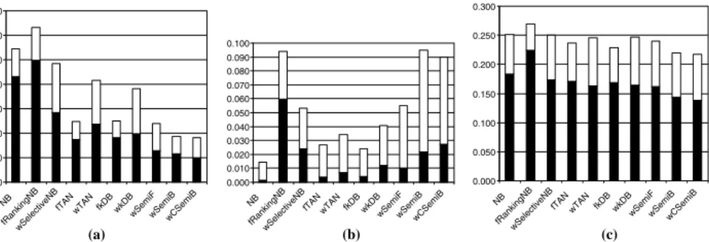
3.4. Bias-variance decomposition of CGN-based classifiers
In this section, we perform the bias-variance decomposition in order to study, in each
Table 5
Bias-variance decomposition of the expected misclassification error rate # Data set Structures
Naive Bayes TAN kDB Semi
NB fRankingNB wSelectiveNB fTAN wTAN fkDB wkDB wSemiF wSemiB wCSemiB
1 BALANCE 6.8 + 3.7 6.0 + 3.3 7.5 + 4.5 7.0 + 4.0 8.2 + 4.1 7.9 + 3.9 7.8 + 3.5 8.5 + 4.9 9.7 + 0.6 8.0 + 3.2 2 BLOCK 6.5 + 2.3 6.1 + 1.9 4.1 + 1.1 5.8 + 1.9 3.1 + 1.4 5.1 + 1.9 3.7 + 2.0 4.2 + 2.6 3.5 + 1.7 3.9 + 2.1 3 BUPA 28.2 + 16.7 47.0 + 0.0 31.3 + 11.6 42.8 + 7.7 25.1 + 18.4 28.5 + 11.5 30.4 + 12.6 35.1 + 11.0 23.6 + 16.7 22.1 + 18.8 4 HABERMAN 28.4 + 1.0 22.5 + 0.0 21.1 + 1.2 29.7 + 3.0 22.3 + 2.2 22.6 + 2.0 18.8 + 3.7 24.1 + 2.3 21.8 + 2.5 21.7 + 2.9 5 HAYES 17.3 + 15.7 19.8 + 19.7 22.2 + 20.4 24.4 + 19.7 35.1 + 15.6 17.6 + 19.6 33.7 + 16.5 24.8 + 20.5 29.9 + 20.0 22.6 + 17.2 6 IRIS 3.5 + 0.9 2.6 + 3.3 3.6 + 2.7 0.4 + 1.7 2.1 + 3.2 2.4 + 1.6 6.2 + 1.3 2.5 + 2.7 2.8 + 1.1 4.1 + 2.1 8 LIVER 27.8 + 17.8 41.7 + 0.0 37.5 + 10.9 24.4 + 14.8 29.8 + 12.5 40.4 + 10.1 25.8 + 17.8 33.0 + 14.3 22.7 + 15.7 25.9 + 14.6 9 PIMA 21.9 + 3.6 31.0 + 1.6 18.9 + 4.5 21.7 + 5.5 19.0 + 5.6 21.5 + 5.1 22.6 + 5.3 20.4 + 5.5 19.6 + 6.1 18.9 + 7.5 10 VEHICLE 43.1 + 11.4 49.7 + 13.6 28.4 + 19.9 17.4 + 7.3 23.7 + 17.7 18.2 + 6.7 19.8 + 18.5 12.9 + 11.0 11.7 + 7.0 10.0 + 8.1 11 WAVEFORM 18.1 + 0.7 13.9 + 3.6 13.9 + 4.7 14.6 + 3.4 10.6 + 7.1 13.1 + 4.4 10.9 + 6.8 11.6 + 6.4 10.9 + 4.9 11.8 + 4.7 12 WINE 0.1 + 1.3 6.0 + 3.4 2.4 + 2.9 0.4 + 2.3 0.7 + 2.7 0.4 + 2.0 1.2 + 2.9 1.0 + 4.5 2.2 + 7.3 2.7 + 6.3 Average 18.3 + 6.8 22.4 + 4.6 17.4 + 7.7 17.1 + 6.5 16.3 + 8.2 16.2 + 6.3 16.4 + 8.3 16.2 + 7.8 14.4 + 7.6 13.8 + 8.0 A. Pe ´rez et al. / Internat. J. Approx. Reason. 43 (2006) 1–25
classifiers presented. The bias-variance decomposition can be useful to explain the
behav-iors of the different algorithms[59]. The concept of bias-variance decomposition was
intro-duced to machine learning for mean squared error by German et al.[21]. Later versions for
zero-one-loss functions were given by Friedman[16], Kohavi and Wolpert[36], Domingos
[9]and James[28].
The decompositions have been performed following Kohavi and Wolpert’s proposal
[36] with parameters N= 20 and m= 1/3jBDj, where N is the number of training sets,
mis its size andjBDjis the size of the data set. We have setN= 20 because the bias
esti-mation is precise enough for this value (seeFig. 1 of[36]), and m= 1/3jBDjto ensure a
minimum training set size which could avoid overfitting problems. Kohavi and Wolpert choose a set of databases with at least 500 instances in order to ensure accurate estimates
of the error. In order to interpret the results, we must take into account that only the
BAL-ANCE,BLOCK,PIMA,VEHICLEandWAVEFORMdata sets fulfill this condition (see
Table 1). Thus, the conclusions obtained with the data sets mentioned are the most impor-tant ones.
The bias-variance decomposition proposed in[36] is as follows:
E¼X x PðxÞðr2 xþbias 2 xþvarxÞ ð8Þ
wherexis an instance of the test set,r2
x is the ‘‘intrinsic’’ target noise,bias
2
x is the square
bias and varx is the variance associated with instance x. bias2¼PxPðxÞbias
2 x and
var¼PxPðxÞvarxare the averaged squared bias and variance (or bias and variance terms
of the decomposition). The target noise is the expected cost of the Bayes-optimal classifier. Therefore, it is independent of the learning algorithm. In practice, if there are two in-stances in the test set with the same configuration for the predictors and a different value
for the class, the estimated ‘‘intrinsic’’ noise is positive, otherwise is zero[36]. Thus, it is
considered zero given the data sets selected. The bias component can be seen as the error due to the incorrect fitness of the hypothesis density function (modeled by the classifier) to the target density function (the real density of the data). On the other hand, the variance component measures the variability of the hypothesis function, which is independent of the target density function. It can be seen as a measure of the learning algorithm’s sensi-tivity to changes in the training set. From these concepts, we can hypothesize that bias and variance terms become lower and higher, respectively, as the number of parameters needed to model the classifier grows (as classifier complexity increases).
0.000 0.100 0.200 0.300 0.400 0.500 0.600 0.700 NB fRankingNB wSelectiveNB
fTAN wTAN fkDB wkDBwSemiFwSemiB wCSemiB (a) 0.000 0.010 0.020 0.030 0.040 0.050 0.060 0.070 0.080 0.090 0.100 NB fRankingNB wSelectiveNB
fTAN wTAN fkDB wkDBwSemiFwSemiB wCSemiB (b) 0.000 0.050 0.100 0.150 0.200 0.250 0.300 NB fRankingNB wSelectiveNB
fTAN wTAN fkDB wkDBwSemiFwSemiB wCSemiB
(c)
Fig. 4. Bias-variance decomposition examples. (a)VEHICLEdata set. (b)WINEdata set. (c) Average across all data sets.
Table 5shows the results of the decomposition obtained for each classifier in each data set. It also includes an additional row which contains the averages for each classifier across
all data sets. For example fTAN obtains abias2= 7.0 and var= 4.0 decomposition for
BALANCE, and an average decomposition across all the data sets of bias2= 17.1 and
var= 6.5.
FromTable 5, one can conclude, in general, that the bias terms of the CGN-based clas-sifiers presented are higher than the variance term. This can be due to the low number of parameters needed to model even the most complex classifiers, which can be interpreted as
low sensitivity. Besides, it can be seen that, on average (see row Average ofTable 5and
Fig. 4(c)), the bias term decreases with an increase of model complexity, whereas the var-iance remains almost constant.
In order to illustrate the behavior of the classifiers taking into account the different
complexities, two different behaviors must be underlined. They are illustrated in Figs.
4(a) and (b) respectively (which correspond to the rows labeled with VEHICLE and
WINEofTable 5).Fig. 4(a) shows that the bias term decreases if the complexity increases. This could be due to the great adjustment of the more complex models, which can approx-imate the target densities better. The variance term is always lower than the bias. Finally, the variance of the filter algorithms seems to be slightly lower compared to the wrapper algorithms.
Fig. 4(b) shows the opposite behavior for the bias term: it grows if complexity grows. On the other hand, the variance shows an erratic behavior. This could be due to the overfit of the train set (WINE has only 179 cases and, besides, it can be considered an easy data set). It must also be highlighted that only in WINE is the variance of most of the algo-rithms higher than the bias term. As we explained before, the behavior of the average
across all the data sets at each algorithm, shown inFig. 4(c), is consistent with the
behav-ior inFig. 4(a): the bias term decreases with the complexity whereas the variance remains
almost constant.
4. Conclusions and future work
In this work, a battery of filter and wrapper classifiers, based on CGNs, is proposed to deal with continuous variables. We have adapted, from the BMN to the CGN paradigm, the following algorithms: naive Bayes, selective naive Bayes, filter tree augmented
net-work, wrapper tree augmented netnet-work, filterk-dependencies Bayesian classifier, wrapper
semi naive Bayes forward, and wrapper semi naive Bayes backward. Three novel
algo-rithms have also been proposed:filter ranking naive Bayes,wrapper k-dependence Bayesian
classifierandwrapper condensed semi naive Bayes backward. Besides, in order to make the
filter algorithms possible, two new results for mutual information are introduced for
Gaussian distributed variables.
The classifiers have been compared in twelve data sets by means of the estimated
pre-dictive accuracy. In short, taking into account the data sets included, the family ofsemi
structure-based algorithms obtains the best results with both scores. They also obtain quite
competitive results compared to the state-of-the-art classifiers included. The novel
con-densed semi naive Bayes backwardseems to be the best algorithm for classification, taking
into account the analysis of Section3. wSemiF and wSemiB behave like wCSemiB. The
competitive results of the novelwrapper k-dependence Bayesian classifier should also be
The behavior of the bias and variance terms in the expected error rate decomposition
[36]shows that, if the model complexity increases, the bias term decreases and the variance
remains constant.
A future work line, related to the wrapper approach, consists in adapting more classi-fiers supported by BMN to directly operate with continuous variables. Randomized
heu-ristics (such asgenetic algorithms[23]or estimation distribution algorithms[41]) could be
used as the search engine in the space of classifier structures.
Acknowledgements
This work was supported in part by a PhD purpose grant from the Basque Government for the first author, by the SAIOTEK-S-PE04UN25 and ETORTEK-bioGUNE 2005 pro-jects from the Basque Government and TIN2005-03824 project from the Spanish Ministry of Education and Science. We also thank the comments of the anonymous reviewers which helped us to improve the quality of this work.
References
[1] F.W. Anderson, An Introduction to Multivariate Statistical Analysis, John Wiley and Sons, 1958. [2] S.G. Bottcher, Learning Bayesian networks with mixed variables, PhD thesis, Aalborg University, 2004. [3] E. Castillo, J.M. Gutierrez, A.S. Hadi, Expert Systems and Probabilistic Network Models, Springer-Verlag,
1997.
[4] J. Cheng, R. Greiner, Comparing Bayesian network classifiers, in: Proceedings of the 15th Conference on Uncertainty in Artificial Intelligence, 1999, pp. 101–107.
[5] C. Chow, C. Liu, Approximating discrete probability distributions with dependence trees, IEEE Transactions on Information Theory 14 (1968) 462–467.
[6] T.M. Cover, J.A. Thomas, Elements of Information Theory, John Wiley and Sons, 1991.
[7] T.T. Cover, P.E. Hart, Nearest neighbour pattern classification, IEEE Transactions on Information Theory 13 (1967) 21–27.
[8] M. DeGroot, Optimal Statistical Decisions, McGraw-Hill, New York, 1970.
[9] P. Domingos, A unified bias-variance decomposition and its applications, in: Proceedings of the 17th International Conference on Machine Learning, Morgan Kaufman, 2000, pp. 231–238.
[10] P. Domingos, M. Pazzani, On the optimality of the simple Bayesian classifier under zero-one loss, Machine Learning 29 (1997) 103–130.
[11] R. Duda, P. Hart, Pattern Classification and Scene Analysis, John Wiley and Sons, 1973. [12] E.J. Dudewicz, S.N. Mishra, Modern Mathematical Statistics, John Wiley and Sons, 1988.
[13] M. Egmont-Peterson, Feature selection by Markov chain Monte Carlo sampling: a Bayesian approach, in: Proceedings of the Joint IAPR Workshops SSPR 2004 and SPR 2004, 2004, pp. 1034–1042.
[14] U. Fayyad, K. Irani, Multi-interval discretization of continuous-valued attributes for classification learning, in: Proceedings of the 13th International Conference on Artificial Intelligence, 1993, pp. 1022–1027. [15] R.A. Fisher, The use of multiple measurements, Annals of Eugenics 7 (1936) 179–188.
[16] J.H. Friedman, On bias, variance, 0/1 - loss, and the curse-of-dimensionality, Data Mining and Knowledge Discovery 1 (1997) 55–77.
[17] N. Friedman, D. Geiger, M. Goldszmidt, Bayesian network classifiers, Machine Learning 29 (1997) 131–163. [18] N. Friedman, M. Goldszmidt, T. Lee, Bayesian network classification with continuous attributes: getting the best of both discretization and parametric fitting, in: Proceedings of the 15th National Conference on Machine Learning, 1998.
[19] D. Geiger, D. Heckerman, Learning Gaussian networks, Technical Report, Microsoft Research, Advanced Technology Division, 1994.
[20] D. Geiger, D. Heckerman, Beyond Bayesian networks: similarity networks and Bayesian multinets, Artificial Intelligence 82 (1996) 45–74.
[21] S. German, E. Bienenstock, R. Doursat, Neural networks and the bias-variance dilemma, Neural Computation 4 (1992) 1–58.
[22] P. Giudici, P.J. Green, Decomposable graphical Gaussian model determination, Biometrika 86 (4) (1999) 785–801.
[23] D.E. Goldberg, Genetic Algorithms in Search, Optimization and Machine Learning, Addison-Wesley, 1989. [24] D. Grossman, P. Domingos, Learning Bayesian network classifiers by maximizing conditional likelihood, in:
Proceeding of the 21th International Conference on Machine Learning, 2004.
[25] I. Guyon, A. Elisseeff, An introduction to variable and feature selection, Journal of Machine Learning Research 3 (2003) 1157–1182.
[26] M.A. Hall, L.A. Smith, Feature subset selection: a correlation based filter approach, in: Proceeding of the Fourth International Conference on Neural Information Processing and Intelligent Information Systems, 1997, pp. 855–858.
[27] D.E. Heckerman, D. Geiger, D. Chickering, Learning Bayesian networks: the combination of knowledge and statistical data, Machine Learning 20 (1995) 197–243.
[28] G.M. James, Variance and bias for general loss functions, Machine Learning 51 (2003) 115–135.
[29] T. Jebara, Discriminative, generative, and imitative learning, PhD thesis, Massachusetts Institute of Technology, 2001.
[30] G. John, P. Langley, Estimating continuous distributions in Bayesian classifiers, in: Proceedings of the 11th Conference on Uncertainty in Artificial Intelligence, 1995, pp. 338–345.
[31] R.A. Johnson, D.W. Wichern, Applied Multivariate Statistical Analysis, Prentice-Hall, 2002. [32] I.T. Jolliffe, Principal Component Analysis, Springer-Verlag, 1986.
[33] E.J. Keogh, M. Pazzani, Learning augmented Bayesian classifiers: a comparison of distribution-based and non distribution-based approaches, in: Proceedings of the 7th International Workshop on Artificial Intelligence and Statistics, 1999, pp. 225–230.
[34] R. Kohavi, Wrappers for performance enhancement and oblivious decision graphs, PhD Thesis, Computer Science department, 1995.
[35] R. Kohavi, G. John, Wrappers for feature subset selection, Artificial Intelligence 97 (1–2) (1997) 273–324. [36] R. Kohavi, D.H. Wolpert, Bias plus variance decomposition for zero-one loss functions, in: International
Conference on Machine Learning, 1996.
[37] I. Kononenko, Semi-naive Bayesian classifiers, in: Proceedings of the 6th European Working Session on Learning, 1991, pp. 206–219.
[38] M. Kudo, Comparison of algorithms that select features for pattern classifiers, Machine Learning 33 (1) (2000) 25–41.
[39] P. Langley, W. Iba, K. Thompson, An analysis of Bayesian classifiers, in: Proceedings of the 10th National Conference on Artificial Intelligence, 1992, pp. 223–228.
[40] P. Langley, S. Sage, Induction of selective Bayesian classifiers, in: Proceedings of the 10th Conference on Uncertainty in Artificial Intelligence, 1994, pp. 399–406.
[41] P. Larran˜aga, J.A. Lozano, Estimation of Distribution Algorithms. A New Tool for Evolutionary Computation, Kluwer Academic Publishers, 2002.
[42] S.L. Lauritzen, Graphical Models, Oxford University Press, 1996.
[43] S.L. Lauritzen, N. Wermuth, Mixed interaction models. Technical Report r 84-8, Institute for Electronic Systems, Aalborg University, 1984.
[44] S.L. Lauritzen, N. Wermuth, Graphical models for associations between variables, some of which are qualitative and some quantitative, Annals of Statistics 17 (1989).
[45] H. Liu, H. Motoda, Feature Selection for Knowledge Discovery and Data Mining, Kluwer Academic Publishers, 1998.
[46] M. Minsky, Steps toward artificial intelligence, Transactions on Institute of Radio Engineers 49 (1961) 8–30. [47] P.M. Murphy, D.W. Aha, UCI repository of machine learning databases, Technical Report, University of
California at Irvine, 1995. Available from:<http://www.ics.uci.edu/ ~ mlearn>. [48] R. Neapolitan, Learning Bayesian Networks, Prentice-Hall, 2003.
[49] M. Pazzani, Searching for dependencies in Bayesian classifiers, in: Learning from Data: Artificial Intelligence and Statistics V, 1997, pp. 239–248.
[50] J. Pearl, Probabilistic Reasoning in Intelligent Systems: Networks of Plausible Inference, Morgan Kaufmann Publishers, 1988.