Physically coherent probabilistic weather forecasts using multivariate discrete copula-based ensemble postprocessing methods

(1)

INAUGURAL–DISSERTATION

zur

Erlangung der Doktorwürde

der

Naturwissenschaftlich–Mathematischen Gesamtfakultät

der

Ruprecht–Karls–Universität

Heidelberg

vorgelegt von

Diplom–Mathematiker Roman Schefzik

aus Mannheim

(2)

(3)

Physically coherent probabilistic

weather forecasts using

multivariate discrete copula-based

ensemble postprocessing methods

Betreuer: Prof. Dr. Tilmann Gneiting

Dr. Thordis Thorarinsdottir

(4)

(5)

Abstract

Being able to provide accurate forecasts of future quantities has always been a great human desire and is essential in numerous situations in daily life. Meanwhile, it has become routine to work with probabilistic forecasts in the form of full predictive distributions rather than with single deterministic point forecasts in many disciplines, with weather prediction acting as a key example.

Nowadays, probabilistic weather forecasts are usually constructed from ensemble prediction systems, which consist of multiple runs of numerical weather prediction models diﬀering in the initial conditions and/or the parameterized numerical representation of the atmosphere. The raw ensemble forecasts typically reveal biases and dispersion errors and thus call for statistical postprocessing to realize their full potential. Several ensemble postprocessing methods have been developed and are partly recapitulated in this thesis, yet many of them only apply to a single weather quantity at a single location and for a single prediction hori-zon. In many applications, however, there is a critical need to account for spatial, temporal and inter-variable dependencies.

To address this, a tool called ensemble copula coupling (ECC) is introduced and examined. Essentially, ECC uses the empirical copula induced by the raw ensemble to aggregate sam-ples from predictive distributions for each location, variable and look-ahead time separately, which are obtained via existing univariate postprocessing methods. The ECC ensemble in-herits the multivariate rank dependence pattern from the raw ensemble, thereby capturing the ﬂow dependence.

Several variants and modiﬁcations of ECC are studied, and it is demonstrated that the ECC concept provides an overarching frame for existing techniques scattered in the litera-ture.

From a mathematical point of view, it is shown that ECC can be considered a copula approach by pointing out relationships to multivariate discrete copulas, which are intro-duced in this thesis and for which relevant mathematical properties are derived.

A generalization of standard ECC is introduced, which aggregates samples from not neces-sarily univariate, but general predictive distributions obtained by low-dimensional postpro-cessing in an ECC-like manner.

Finally, the SimSchaake approach, which combines the notion of similarity-based ensem-ble methods with that of the so-called Schaake shuﬄe, is presented as an alternative to ECC. In this technique, the dependence patterns are based on verifying observations rather than on raw ensemble forecasts as in ECC.

The methods and concepts are illustrated and evaluated based on case studies, using real ensemble forecast data of the European Centre for Medium-Range Weather Forecasts. Es-sentially, the new multivariate approaches developed in this thesis reveal good predictive performances, thus contributing to improved probabilistic forecasts.

(6)

(7)

Zusammenfassung

Es ist schon immer ein großes menschliches Bedürfnis gewesen und in zahlreichen Situatio-nen des täglichen Lebens unabdingbar, präzise Vorhersagen zukünftiger Größen bereitstellen zu können. Mittlerweile ist es in vielen Disziplinen zur Gewohnheit geworden, mit proba-bilistischen Vorhersagen in der Form von vollständigen Vorhersageverteilungen zu arbeiten, und nicht mit einzelnen deterministischen Punktvorhersagen, wobei die Wettervorhersage als ein Schlüsselbeispiel fungiert.

Heutzutage werden probabilistische Wettervorhersagen üblicherweise auf der Grundlage von Ensemblevorhersagesystemen erstellt, die aus mehreren Durchläufen numerischer Wetter-vorhersagemodelle bestehen, welche sich hinsichtlich der Anfangsbedingungen und/oder der parameterisierten numerischen Darstellung der Atmosphäre unterscheiden. Die unbearbei-teten Ensemblevorhersagen oﬀenbaren typischerweise systematische und Dispersionsfehler und benötigen daher eine statistische Nachbereitung, um ihr volles Leistungsvermögen zu verwirklichen. Mehrere Nachbereitungsmethoden für Ensembles sind entwickelt worden und werden in dieser Arbeit zum Teil rekapituliert, wobei viele davon jedoch nur für eine einzelne Wettergröße, an einem einzelnen Ort und für einen einzelnen Vorhersagehorizont gelten. In vielen Anwendungen besteht jedoch ein dringender Bedarf, räumliche, zeitliche und Ab-hängigkeiten zwischen den Größen zu berücksichtigen.

Um dies zu bewerkstelligen, wird ein Werkzeug namens Ensemble Copula Coupling (ECC) eingeführt und untersucht. Im Wesentlichen verwendet ECC die von dem unbearbeiteten Ensemble induzierte empirische Copula, um Stichproben von getrennten Vorhersagevertei-lungen für jeden Ort, jede Variable und jeden Vorhersagehorizont zu verbinden, die durch bestehende univariate Nachbereitungsmethoden erhalten werden. Das ECC-Ensemble über-nimmt das multivariate Rangabhängigkeitsmuster des unbearbeiteten Ensembles und erfasst dadurch die Datenabhängigkeit.

Mehrere Varianten und Modiﬁkationen von ECC werden untersucht und es wird demons-triert, dass das ECC-Konzept einen übergreifenden Rahmen für vorhandene Methoden liefert, die in der Literatur verstreut sind.

Aus mathematischer Sicht wird gezeigt, dass ECC als ein Copulaansatz angesehen wer-den kann, indem Beziehungen zu multivariaten diskreten Copulas aufgezeigt werwer-den, die in dieser Arbeit eingeführt und für die relevante mathematische Eigenschaften hergeleitet werden.

Es wird eine Verallgemeinerung des standardmäßigen ECC eingeführt, die Stichproben von nicht notwendigerweise univariaten, sondern allgemeinen Vorhersageverteilungen, die durch niederdimensionale Nachbereitung erhalten werden, auf eine zu ECC ähnliche Weise verbindet.

Schließlich wird die SimSchaake-Methode, welche die Idee der auf Ähnlichkeit basierenden Ensemblemethoden mit der des sogenannten Schaake-Shuﬄes verbindet, als eine Alternative zu ECC vorgestellt. In diesem Verfahren basieren die Abhängigkeitsmuster auf eingetrete-nen Beobachtungen und nicht auf unbearbeiteten Ensemblevorhersagen wie bei ECC.

(8)

reale Ensemblevorhersagedaten vom Europäischen Zentrum für mittelfristige Wettervorher-sage verwendet werden. Im Wesentlichen zeigen die neuen multivariaten Methoden, die in dieser Arbeit entwickelt werden, eine gute Vorhersageleistung und tragen somit zu verbesser-ten probabilistischen Vorhersagen bei.

(9)

Acknowledgments

First of all, I thank my advisors Tilmann Gneiting and Thordis Thorarinsdottir for their supervision of this thesis, including numerous discussions, and their dedication to induct me into the scientiﬁc sphere with all its facets.

The funding of my work by the Volkswagen Foundation within the project “Mesoscale Weather Extremes: Theory, Spatial Modeling and Prediction (WEX–MOP)” and the Ger-man Research Foundation within the Research Training Group (RTG) 1953 “Statistical Modeling of Complex Systems and Processes–Advanced Nonparametric Approaches”, re-spectively, is gratefully acknowledged.

Moreover, the scientiﬁc support by the Faculty of Mathematics and Computer Science of Heidelberg University and the doctoral training within the Heidelberg Graduate School of Mathematical and Computational Methods for the Sciences are appreciated.

Further, I thank the members in the WEX–MOP project and the RTG 1953 as well as my colleagues at the Institute for Applied Mathematics of Heidelberg University and the Heidelberg Institute for Theoretical Studies, respectively, for creating an enjoyable work-ing atmosphere and for fruitful discussions. I am grateful to Michael Scheuerer and Thordis Thorarinsdottir for providing the forecast and observation data employed for the case studies in this thesis, and further to Elena Scardovi, Michael Scheuerer, Nina Schuhen and Thordis Thorarinsdottir for sharing and providing R code. Besides, I thank Michael Denhard, Mar-tin Leutbecher, Annette Möller, Elena Scardovi and the reviewers of my working papers for useful discussions, comments and hints, and Martin Leutbecher in particular for detecting an error in an earlier version of the data set used in this thesis. Moreover, the support of Marion Münster, Dagmar Neubauer and Milanka Stojkovic in administrative issues is acknowledged. Last but not least, I am indebted to my parents and family, my friends and my club mates for their support and for providing distraction from science in my leisure time.

(10)

(11)

Introduction

1.1 Uncertainty quantiﬁcation and probabilistic forecasting

In many applications, decision making relies on potentially high-dimensional output of com-plex computer simulation models. For instance, this applies to weather and climate predic-tions and the management of air quality, wildfires, floods, groundwater contamination or disease spread – just to name a few examples. During the last years, the recognition of the need for uncertainty quantification of such model output has been rising considerably, which is for example witnessed by the foundation of interest groups on this topic within the Amer-ican Statistical Association (ASA) and the Society for Industrial and Applied Mathematics (SIAM), as well as the launch of the SIAM/ASA Journal on Uncertainty Quantification in 2013.

Frequently, the output data are employed to make predictions for uncertain future quanti-ties or events, which has always been a great human desire. Initially, forecasting had been viewed as a purely deterministic issue, in that a prediction used to be a single number. Such point forecasts are partly still issued today, be it for reasons of tradition, reporting require-ments or market mechanisms, for instance, and are also of theoretical interest (Gneiting, 2011a,b). However, it is meanwhile clearly established that forecasts should be probabilistic in nature (Dawid, 1984), having the form of full predictive probability distributions over future quantities or events instead of single-valued point forecasts. That is, in place of stat-ing twenty degrees Celsius (◦C) as a point forecast for temperature at noon in Heidelberg on a spring day, one should rather issue a predictive distribution, for instance a normal distribution with a mean of twenty degrees Celsius and a standard deviation of one degree Celsius. If ever, probabilistic forecasts in former times were made almost only for binary events (Gigerenzer et al., 2005), such as the chance of rain at noon in Heidelberg on a cer-tain day. Nowadays, also probabilistic forecasts for multi-category or continuous variables are of great importance and are required in a vast range of scientiﬁc disciplines comprising weather and climate, hydrology, economics and ﬁnance, politics, preventative medicine and epidemiology, among others (Gneiting and Katzfuss, 2014, and references therein).

The aim of probabilistic forecasting is to create predictive distributions of future quan-tities, from which relevant functionals such as moments, quantiles, prediction intervals or event probabilities can be extracted to quantify the uncertainty of the prediction. In this connection, the concepts of sharpness and calibration play an essential role (Gneiting et al.,

(14)

Figure 1.1: Illustration of the goal of probabilistic forecasting: Normal PDFs for temperature in Heidelberg at noon on a spring day made by Forecaster 1 (green curve) and Forecaster 2 (orange curve), respectively. Provided that both predictive distributions are calibrated, the sharper one by Forecaster 1 should be preferred.

centration of the predictive distributions. Calibration, on the other hand, is a joint property of the probabilistic forecasts and the observations, referring to the statistical compatibil-ity between them, in the sense that events predicted to occur with probabilcompatibil-ity p should materialize with empirical frequency p. Gneiting et al. (2007) contend that predictive dis-tributions should be as sharp as possible, subject to calibration. For instance, let the green and orange curves in Figure 1.1 be normal predictive probability density functions (PDFs) for temperature in Heidelberg at noon on a spring day made by Forecaster 1 (green curve) and Forecaster 2 (orange curve), respectively. In this case, the two predictive distributions have the same location, but that issued by Forecaster 1 is sharper, as it obviously reﬂects a lower degree of uncertainty than that issued by Forecaster 2. The predictive distribution according to Forecaster 1 should thus be preferred, provided that both forecast distributions are calibrated.

From now on, we concentrate on weather prediction as a key application area of proba-bilistic forecasting for the rest of the thesis. However, it should always be kept in mind that the presented concepts and methods may also apply in much broader settings in which uncertainty is to be quantiﬁed.

1.2 Weather prediction and ensemble postprocessing

Accurate predictions for future weather quantities or events are of crucial interest in our society for various reasons. For instance, they become valuable when warnings about ex-treme events or natural catastrophes such as inundations, storms or droughts are sought. In times in which alternative energy sources become more and more important, they may also aﬀect decisions regarding energy generation through solar technology or wind power plants. Finally, weather forecasts may simply help to facilitate the organization of one’s leisure time activities.

(15)

beginning of the 20th century. Essentially, Bjerknes (1904) proposed the possibility of nu-merical weather prediction (NWP), stating that the physics of the atmosphere at any point in time can be determined based on seven equations in seven parameters, namely the three hydrodynamic equations of motion (conservation of momentum), the continuity equation (conservation of mass during motion), the equation of state for the atmosphere and the two fundamental laws of thermodynamics (conservation of energy and entropy), comprising three velocity components, density, pressure, temperature and humidity. From a present-day per-spective, Bjerknes actually should have rather issued a continuity equation for water than the second thermodynamic law (Lynch, 2008). According to Bjerknes (1904), solving the equation of state eliminates one of the seven unknowns. The remaining equations then build a system of six partial differential equations in six variables, where the initial conditions are set by the observations of the initial state of the atmosphere. As Bjerknes himself did not put his procedure into practice, it was Richardson who derived by hand the first weather prediction more than a decade later, employing a finite differences approach (Richardson, 1922) to simplify the equations in Bjerknes (1904). Unfortunately, his attempts were highly unsatisfactory, both with respect to the totally unrealistic forecast values themselves and the extraordinarily high calculation time needed. However, the advent of the computer sparked hopes to lead Richardson’s preparatory work to success, with von Neumann demanding to use computers for weather prediction in 1946. Finally, the first weather forecast made by a computer was issued by the Electronic Numerical Integrator and Computer (ENIAC) of the United States Army in 1950. The first operational forecasts, that is, routine predictions for practical use, were generated by Rossby’s group in Sweden in 1954 (Harper et al., 2007). From then on, work on NWP models has continuously intensified, in that new atmospheric models have been introduced and the size of the initial data sets has grown, to take advan-tage of the increasing computer power in the second half of the 20th century. Moreover, data assimilation systems, which supply the initial conditions describing the current state of the atmosphere on a three-dimensional grid, have become more powerful. For a more detailed overview of the development and the history of NWP, we refer to Harper et al. (2007) and Lynch (2008).

Nowadays, NWP models are still based on a system of partial diﬀerential equations, which are discretized and run forward in time to achieve deterministic forecasts of future atmo-spheric states, and form the basis of modern weather forecasting. However, they exhibit two major sources of uncertainty:

1. The initial conditions might be inaccurate due to incomplete observation data, deﬁ-ciencies in data assimilation or measurement errors, for example.

2. The model formulation might be inaccurate due to incomplete or inadequate numerical schemes or imperfect knowledge of physical processes including inaccurate parameter-izations of sub grid-scale processes, for instance.

Hence, there is an obvious need for uncertainty quantiﬁcation in weather forecasts. This had already been recognized at the beginning of the 20th century by Cooke (1906, page 23), stating that

“All those whose duty is to issue regular daily forecasts know that there are times when they feel very conﬁdent and other times when they are doubtful as to the coming weather. It seems to me that the condition of conﬁdence or otherwise

(16)

Lorenz (1963) pointed out the non-linear, chaotic nature of the equations involved in NWP models, in that extremely small deviations in initial inputs might lead to largely differing evolutions of the model – an observation which has later become famous as the “butterfly effect” (Lorenz, 1993). Thus, it becomes impossible to definitely predict the state of the atmosphere. Epstein (1969) stated that it is not appropriate to describe the atmosphere via only a single forecast run and introduced an ensemble of stochastic Monte Carlo simulations to generate means and variances for the atmospheric state, which can be viewed as an early example of probabilistic weather forecasting.

Nevertheless, weather prediction had been considered a deterministic issue through the 1980s, with the idea that for a set of “best” input data, the NWP model leads to one “best” deterministic weather forecast (Gneiting and Raftery, 2005). However, in the early 1990s, a radical change of mind took place in the meteorological community, in that weather fore-casts for future quantities or events are now preferred to take the form of full predictive probability distributions rather than single-valued deterministic point forecasts.

The most convenient way to achieve a probabilistic weather prediction is based on so-called ensemble prediction systems of NWP forecasts (Palmer, 2002; Gneiting and Raftery, 2005). An ensemble consists of multiple runs of NWP models diﬀering in the initial conditions and/or the model formulation with respect to the parameterized numerical representation of the atmosphere, thereby addressing the above-mentioned two major sources of uncer-tainty. Combinations of ensemble member forecasts frequently show more accuracy than any of these forecasts separately (Palmer, 2002). Interpreting ensemble forecasts as a sample from the predictive distribution allows weather forecasts to become probabilistic.

Ensemble prediction systems have been employed operationally since 1992 and can be run either globally or over limited areas. Examples for global ensembles include those run by the European Centre for Medium-Range Weather Forecasts (ECMWF) (Molteni et al., 1996; Buizza, 2006; Leutbecher and Palmer, 2008; ECMWF Directorate, 2012) and the National Centers for Environmental Predictions (NCEP) (Toth and Kalnay, 1997), respectively, while the University of Washington Mesoscale Ensemble (UWME) (Eckel and Mass, 2005) and the COSMO-DE ensemble of the German Weather Service (Gebhardt et al., 2011) are represen-tatives of limited area systems. Moreover, there are single-model and multi-model ensemble prediction systems. A single-model ensemble is based on one particular NWP model, and the diﬀerent ensemble forecasts are obtained by perturbing the initial conditions and pa-rameterizations. On the contrary, a multi-model ensemble is an aggregation of single-model ensembles, as for instance in the THORPEX Interactive Grand Global Ensemble (TIGGE) database (Bougeault et al., 2010) provided by leading weather centers.

Ensemble members can be regarded as exchangeable (Bröcker and Kantz, 2011) if they differ in random perturbations only, such that they lack individually distinguishable physi-cal features and are statistiphysi-cally indistinguishable. For example, ensembles with exchange-able members can be generated by using bred vectors as in the NCEP ensemble, singular vectors as in the ECMWF ensemble, or ensemble Kalman filter systems (Evensen, 1994; Hamill, 2006). On the other hand, an ensemble prediction system is considered to consist of non-exchangeable members if the NWP inputs or the model parameterizations differ in a systematic rather than a random fashion. An example for an ensemble system with non-exchangeable members is the COSMO-DE ensemble run by the German Weather Service.

(17)

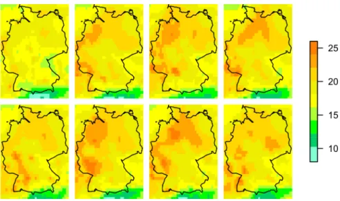
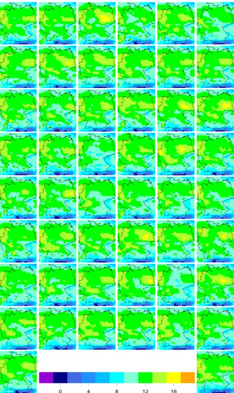
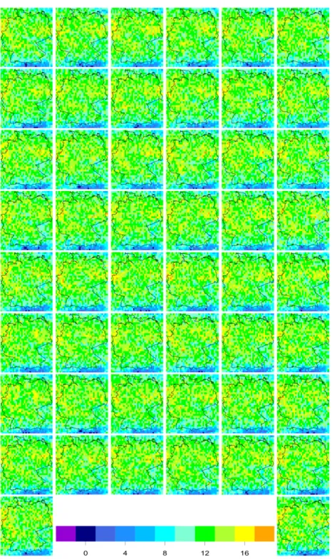
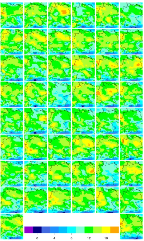
Figure 1.2: 24 hour ahead ensemble forecast for temperature (in ◦C) over Germany, valid 2:00 am on 3 July 2010. Eight randomly selected members of the ECMWF ensemble are shown.

An illustration of a 24 hour ahead ensemble forecast for temperature over Germany, valid at 2:00 am on 3 July 2010, is given in Figure 1.2, where eight out of the 50 exchangeable members of the ECMWF ensemble are shown. The ECMWF is one of the leading NWP centers worldwide, and its global 50-member ensemble prediction system (Molteni et al., 1996; Buizza, 2006; Leutbecher and Palmer, 2008; ECMWF Directorate, 2012), which will be described extensively in the next section, has been operational since 1992.

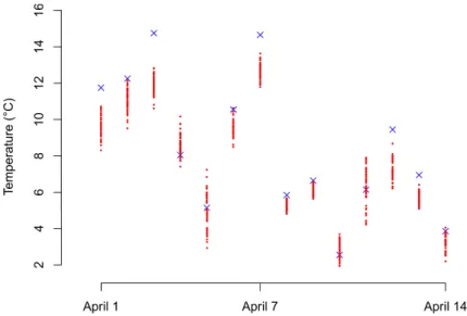
The aim of NWP ensemble systems is to address the inherent uncertainty in the prediction. Ensemble forecasts often exhibit a spread-error association, in that a positive correlation between the ensemble range and the forecast error can be observed. The ensemble spread oﬀers an estimate of the uncertainty of the forecast. While on some days, the ensemble spread might be small and the atmosphere thus rather predictable, the ensemble forecasts might diverge drastically on other days, indicating an extremely unpredictable atmosphere. Despite their beneﬁts, the raw NWP ensemble forecasts however tend to reveal model biases and dispersion errors (Hamill and Colucci, 1997). While a model bias refers to systematic errors in the NWP forecast, dispersion errors essentially mean a lack of calibration, in that the observed values fall far too often outside the ensemble ranges, contrary to the desired statistical compatibility between observations and forecasts. An example is given in Figure 1.3, where the 24 hour ahead 50-member ECMWF ensemble forecasts (red dots) for tem-perature at Hamburg along with the corresponding verifying observations (blue crosses) are shown for the period from 1 April 2011 to 14 April 2011, valid at 2:00 am each day.

To cope with biases and lack of calibration, the NWP raw ensemble forecasts call for statis-tical postprocessing, which targets at creating calibrated and sharp predictive probability distributions. During the last decade, several univariate ensemble postprocessing methods have been proposed, with Bayesian model averaging (BMA) (Raftery et al., 2005, for in-stance) and ensemble model output statistics (EMOS) (Gneiting et al., 2005, for example), which is also known as non-homogeneous regression, being two of the most prominent ones.

(18)

Figure 1.3: 24 hour ahead 50-member ECMWF ensemble forecasts for temperature at Hamburg (red dots) and corresponding verifying observations (blue crosses), valid 2:00 am for the period from 1 April 2011 to 14 April 2011.

to a kernel function, using a weight which reﬂects the member’s relative skill. The EMOS method ﬁts a single, parametric PDF in a regression setting, using summary statistics from the ensemble. Figure 1.4 shows an example of a 24 hour ahead EMOS predictive PDF for temperature at Hamburg, valid at 2:00 am on 1 April 2011. The vertical red lines indi-cate the 50 ECMWF raw ensemble values, the vertical line of blue crosses the verifying observation, and the vertical black lines the 10th, 50th and 90th percentiles, respectively, of the EMOS distribution. The EMOS predictive distribution corrects both a negative bias and underdispersion. BMA and EMOS postprocessing techniques have been developed for various weather variables and turn out to be well performing, but they mostly apply to a single weather quantity at a single location and a single prediction horizon only.

This is very unfortunate, as in many applications such as flood management, air traffic control, ship routing or winter road maintenance, it is crucially relevant to account for spatial, inter-variable and temporal dependence structures, which cannot be handled by in-dependently postprocessed forecasts. Hence, there is a critical need for multivariate methods that provide physically realistic and coherent probabilistic forecasts for multiple locations, weather quantities and prediction horizons simultaneously. Consequently, much effort has been invested to address this challenge in the last years, and several ensemble postprocessing approaches being able to account for multivariate dependence structures have emerged. Ex-amples include the Spatial BMA approach of Berrocal et al. (2007) and the Spatial EMOS method of Feldmann et al. (2014) for purely spatial settings dealing with temperature and the Gaussian copula method of Möller et al. (2013) to handle inter-variable dependencies. The techniques of Pinson (2012), Schuhen et al. (2012) and Sloughter et al. (2013), respec-tively, aim particularly at the postprocessing of wind vectors. These methods are parametric and perform well in low-dimensional situations and if specific structure can be exploited.

Frequently, statistical postprocessing of a full NWP ensemble forecast forms a very high-dimensional challenge. For example, one might be confronted with ﬁve weather quantities at 500×500 grid boxes and ten vertical levels for 72 lead times, yielding a total of 900 million

(19)

Figure 1.4: 24 hour ahead EMOS predictive PDF for temperature at Hamburg, valid 2:00 am on 1 April 2011. The vertical red lines indicate the 50 ECMWF raw ensemble values, the vertical line of blue crosses the verifying observation, and the vertical black lines the 10th, 50th and 90th percentiles, respectively, of the EMOS distribution.

variables. Even if not all of them might need to be treated simultaneously, many applica-tions comprise much higher dimensions than can be adequately treated by parametric mod-els. Hence, the use of non-parametric techniques, such as the Schaake shuffle (Clark et al., 2004), appears to be most beneficial in high-dimensional settings. Against this background, a multi-stage non-parametric procedure called ensemble copula coupling (ECC) (Schefzik et al., 2013) to handle spatial, inter-variable and temporal dependencies is proposed in this thesis. The key idea is that the postprocessed ECC forecast ensemble inherits the spatial, temporal and inter-variable correlation pattern of the unprocessed raw ensemble, thereby honoring the flow dependence. Basically, this is achieved by using the empirical copula of the raw ensemble to aggregate samples from predictive distributions obtained by univariate postprocessing techniques, which is why ECC can be considered a discrete copula-based approach. ECC requires negligible computational effort once the univariate postprocess-ing is done, and in concert with its theoretical discrete copula background, it turns out to form an overarching frame for existing techniques scattered in the literature. Moreover, the ECC notion appears to be particularly appealing as it combines analytic, numerical and statistical modeling and can be applied not only to weather prediction, but also in broader settings, in which uncertainty quantification is required. In this thesis, we discuss several variants and modifications of ECC and relate ECC to the Schaake shuffle (Clark et al., 2004). To illustrate and test our methods, we apply them to the ECMWF ensemble in real-data case studies. For that reason, a detailed description of the ECMWF ensemble dataset as employed in this thesis is provided in the following section.

1.3 The European Centre for Medium-Range Weather

Fore-casts (ECMWF) ensemble

The European Centre for Medium-Range Weather Forecasts (ECMWF) (http://www.ecmwf. int) is one of the world’s leading weather centers. It it an independent and intergovernmen-tal organization, which is supported by various European member states and co-operating

(20)

Having been established in 1975, the ECMWF’s main objectives comprise the design of nu-merical methods for medium-range weather forecasting, the distribution of the forecasts to the member states, the conduction of research to improve the forecasts, as well as the col-lection and storage of weather data, actually providing the world’s largest archive of NWP data (Woods, 2006).

Since 1992, the ECMWF has been running an ensemble prediction system operationally. The global ECMWF ensemble consists of 50 members and operates at a horizontal reso-lution of approximately 32 kilometers on a 0.25×0.25 degree grid, with lead times up to ten days ahead (Molteni et al., 1996; Buizza, 2006; Leutbecher and Palmer, 2008; ECMWF Directorate, 2012). It produces forecasts twice a day at 00:00 Universal Coordinated Time (UTC) and 12:00 UTC, respectively. The 50 ensemble members can be considered exchange-able, as differences between them arise from random perturbations in initial conditions and stochastic model parameterizations. More precisely, the random perturbations in the ini-tial conditions are generated by using singular vectors, while the model uncertainties are represented by stochastically perturbed parameterization tendencies (Buizza et al., 1999; Palmer et al., 2009). Additionally, the ECMWF provides a so-called control run, which is a distinguished NWP run outside the 50-member ensemble, representing the single-valued best estimate of the atmospheric state at the initialization time due to recent and concurrent observations. Essentially, the 50 ECMWF ensemble member forecasts start from slightly different states being close, but not identical, to the best guess of the initial atmospheric state offered by the control run. In some former case studies in the literature, the control run has been included in the ECMWF ensemble, then comprising 51 members. However, we do not proceed so in this thesis and stick to the 50-member ensemble, partly employing the control run as a reference data set as explained later.

In this thesis, we employ the ECMWF ensemble forecasts initialized at 00:00 UTC only, and we conﬁne ourselves to prediction horizons of 24, 48, 72 and 96 hours, respectively. As we focus on forecasts over Germany, the meteorological format of 00:00 UTC corresponds to local times of 1:00 am in Central European Time and 2:00 am in Central European Summer Time, respectively. The weather variables which will be investigated involve temperature, pressure, precipitation and wind vectors. In this context, a wind vector can be either rep-resented by wind speed and wind direction or equivalently by its u (zonal or west-east) and v (meridional or north-south) velocity components. We use the latter representation in our case studies and refer to u- andv-wind, respectively, in what follows. For pressure, precipitation and (u, v)-wind vectors, we use the corresponding ECMWF ensemble forecasts initialized between 1 February 2010 and 30 April 2011 to build our database. In case of tem-perature, ECMWF ensemble forecast data were available for initializations from 1 February 2010 to 31 December 2012.

Mostly, we focus on the predictive performance of forecasts at the three international airports at Berlin-Tegel, Hamburg-Fuhlsbüttel and Frankfurt am Main. As the ECMWF ensemble forecasts are available on a grid, they need to be bilinearly interpolated to the locations at Berlin, Hamburg and Frankfurt, respectively, before comparing them with the verifying ob-servations, which are directly measured at the three speciﬁc observation sites. However, in some cases, we are also interested in the predictive performance on the whole model grid or at least on test regions over the grid. As there are no verifying observations available for all grid points involved, we use the control run for the prediction horizon of 0 hours initialized

(21)

at the target date as a grid-based ground truth instead, both as training data and for the assessment of predictive performance. For example, 48 hour ahead ensemble forecasts ini-tialized at 00:00 UTC on 1 May 2010 and thus valid at 00:00 UTC on 3 May 2010 would be compared to the ground truth composed of the 0 hour ahead control run nowcast initialized at 00:00 UTC on 3 May 2010, where the term “nowcast” is generally employed for short-term weather predictions with look-ahead times from zero to six hours. As an alternative to the control runs used in this thesis, so-called analyses could be employed as a grid-based veri-fication data set and ground truth, respectively, as is described in Box A in Hagedorn (2010). Principally, we use the one-year test period from 1 May 2010 to 30 April 2011 to assess our methods in case studies and employ forecasts and observations prior to 1 May 2010 as training data. When only temperature is involved, and no comparison to other weather vari-ables is intended, we occasionally take advantage of the corresponding larger database and evaluate our approaches over a longer test period. Our real-data case studies should in fact be rather viewed as illustrations or proof-of-concepts, respectively, as we use comparably small test periods and consider forecasts for few locations, weather variables and look-ahead times, which may not suffice for conclusive statements about predictive performance. The rest of the thesis is organized as follows. In Chapter 2, we give an overview of uni-and multivariate verification methods to assess predictions. Essentially, those tools are pre-sented that are employed later to evaluate the predictive skill in our case studies. Chapter 3 reviews uni- and multivariate statistical ensemble postprocessing methods, with the focus on techniques that are either directly used or needed for comparative reasons in the course of the thesis. The pivotal ensemble copula coupling (ECC) approach, including several vari-ants and modifications, is then introduced in Chapter 4. Chapter 5 shows to what extent ECC can be interpreted as an overarching frame for existing techniques in the literature, whereas the mathematical background of the ECC method in the form of discrete copulas is discussed in Chapter 6. Chapter 7 aims at combining low-dimensional ensemble postpro-cessing methods in an ECC-like manner. In Chapter 8, an alternative approach to ECC based on a combination of similarity-based ensemble methods and the Schaake shuffle is described. Finally, the dissertation closes with a summary and a discussion of the essential results, as well as an outlook on possible future work, in Chapter 9. The proposed methods will be accompanied by illustrative case studies using the ECMWF ensemble throughout the whole thesis.

A very ﬁrst version of the ECC approach from Section 4.1, together with initial case studies, had already been presented in the diploma thesis of Schefzik (2011). The ECC notion will be discussed in much more detail in this thesis here, with much more comprehensive case studies. Similarly, the origin of Chapter 6 about discrete copulas lies in Schefzik (2011), but again, the presentation in this thesis will be more detailed, providing new insights, with a focus on general multivariate settings.

This dissertation is partly based on two research papers. Speciﬁcally, the already pub-lished paper of Schefzik et al. (2013) forms the basis of Chapter 4, while the results of Chapter 6 stem from the working paper of Schefzik (2013), which is available online.

(22)

(23)

Chapter 2

Forecast veriﬁcation methods

In this chapter, we address the question how to evaluate predictions. As already hinted at in the introductory chapter, forecasts essentially can either be issued as single-valued point predictions or as ensemble predictions or as probabilistic forecasts taking the form of a full predictive probability density function (PDF) or cumulative distribution function (CDF), respectively. In this context, an M-member ensemble forecast x1, . . . , xM ∈ Rcan also be

interpreted as a probabilistic forecast for a real-valued quantity in form of a discrete sample, and each sample value can be regarded as an equally likely potential realization of the future outcome. Then, the ensemble forecastx1, . . . , xM can be identiﬁed with its empirical CDF

F given by F(z) := 1 M M m=1 1{xm≤z}

forz∈R, with1_A denoting the indicator function of the eventA.

The diﬀerent forecast formats can be converted to some extent into each other. Ensem-ble predictions or predictive densities can be transformed into point forecasts if necessary or desired by extracting relevant functionals from the corresponding distributions, such as the mean or the median. Moreover, we can always sample from a predictive PDF to obtain an ensemble forecast, and conversely, an ensemble forecast could be replaced by a density estimate, especially if the ensemble size is rather large. Hence, the distinction between en-semble predictions and full forecast PDFs arguably becomes artiﬁcial to a certain degree (Gneiting et al., 2008). Other forecast formats, such as interval predictions, are generally feasible, but are not discussed in this thesis.

In the case of point predictions (Gneiting, 2011a), forecast quality is usually measured on the basis of accuracy and association (Fricker et al., 2013). Accuracy describes the cor-respondence between a forecastx∈Rand an observation y ∈Rand is often quantiﬁed by some function of the error magnitude. Typical examples of such functions include the abso-lute error (AE) given by AE :=|x−y|and the squared error (SE) given by SE := (x−y)2_. In contrast, association measures the extent of a given relationship between forecasts and observations. For instance, Pearson’s correlation coeﬃcient can be employed to quantify the strength of a linear relationship. As this thesis focuses on ensemble and probabilistic forecasts, we do not provide more detail about point forecasts, although relationships might be discussed occasionally.

(24)

calibration, which is sometimes also referred to as reliability, and sharpness. Calibration is a joint property of the predictions and the observations, basically relating to the statistical compatibility between them, whereas sharpness describes the concentration of the predic-tive distributions, thus being a property of the forecasts only. The goal of probabilistic forecasting is to maximize the sharpness of the predictive distributions, subject to calibra-tion (Gneiting et al., 2007). While we will consider calibracalibra-tion and sharpness from a rather applied point of view (Wilks, 2011) in this thesis, a measure-theoretic handling of these concepts in the frame of prediction spaces is provided in Gneiting and Ranjan (2013). Several methods to assess the calibration and the sharpness of ensemble or density fore-casts have been developed, both for the univariate and the multivariate case. Moreover, proper scoring rules have been shown to oﬀer an appealing tool to evaluate calibration and sharpness simultaneously. In view of their utilization in the case studies throughout the thesis, a selection of those evaluation techniques is reviewed in what follows.

2.1 Calibration

As already stated, calibration relates to the statistical compatibility between forecasts and observations, therefore being a joint property of those. Basically, the forecasts are cali-brated if events predicted to occur with probability p materialize with frequency p, or in other words, if the verifying observations can be considered as random draws from the pre-dictive distributions.

In univariate settings, calibration is frequently diagnosed by using the veriﬁcation rank (VR) (Anderson, 1996; Talagrand et al., 1997; Hamill, 2001) in the case of ensemble fore-casts or the probability integral transform (PIT) (Dawid, 1984; Diebold et al., 1998; Gneiting et al., 2007) in case of forecast densities, with reliability diagrams (Wilks, 2011) providing an alternative. The VR is the rank of the materializing observation when pooled with the corresponding M ensemble forecast values. Accordingly, the PIT is the value which the corresponding predictive CDF attains at the verifying observation. Adaptations of the PIT for discrete distributions are proposed in Czado et al. (2009).

Calibration can then be checked empirically by plotting the VR histogram or PIT his-togram for aggregated forecast cases. If a predictive distribution is calibrated, the VR or the PIT are uniformly distributed on{1, . . . , M + 1}or the unit interval [0,1], respectively, and deviations from uniformity in the histograms indicate miscalibration. VR and PIT histograms can be compared directly, and different forms of deviation from uniformity may hint at different reasons for that. For instance, a skew in the histogram indicates biases, a U-shape points at underdispersion, and an inverse U-shape suggests overdispersion in the forecast distributions. Such VR or PIT histograms have been widely used as tools for as-sessing calibration. However, their uncritical employment might yield to misinterpretations of the forecast quality (Hamill, 2001). In particular, Hamill (2001) argues that a flat his-togram does not necessarily indicate a calibrated ensemble. Hence, uniformity is a necessary condition for calibration, but not a sufficient one.

Concerning multivariate situations of dimension L ≥ 2, we focus on evaluation tools for

M-member ensemble forecasts, as this is the format to be dealt with in the methods and case studies later. Speciﬁcally, the multivariate rank (MR) (Gneiting et al., 2008), the band

(25)

depth rank (BDR) (Thorarinsdottir et al., 2014) and the average rank (AR) (Thorarinsdot-tir et al., 2014) provide distinct approaches to rank multivariate data and are employed for calibration veriﬁcation in this thesis. To describe these concepts, letS :={x0,x1, . . . ,xM}

denote the pooled set consisting of the ensemble forecastx1, . . . ,xM ∈RLand the respective

verifying observationx0:=y∈RL, wherexm := (x1m, . . . , xLm)∈RL form∈ {0,1, . . . , M}.

According to Gneiting et al. (2008) and Thorarinsdottir et al. (2014), the rank of the ob-servation inS is then derived in two steps, by

(i) applying a pre-rank functionρ_S :RL_→_R

+to compute the pre-rankρS(xm) for every

m∈ {0,1, . . . , M}and

(ii) setting the rank of x0 equal to the rank of ρS(x0) in {ρS(x0), ρS(x1), . . . ,

ρ_S(x_M)}, where ties are resolved at random.

In this context, the forecasts and observations inS do not need to be standardized, as the rankings in the pre-rank functions considered below operate componentwise, thus being in-variant to such transformations.

In the case of the multivariate rank (MR) (Gneiting et al., 2008), the pre-rank function is deﬁned by ρMR_S (x_m) := M μ=0 1{xμxm}, with the multivariate partial orderingx_μx_m if and only ifx

μ≤xm for all∈ {1, . . . , L}.

The ﬁnal MR is then derived according to (ii), and aggregating the MRs over forecast cases leads to an MR histogram, similarly to the univariate case. Conveniently, the interpreta-tion of the form of the resulting MR histograms coincides with that for the VR or PIT histograms in the univariate case discussed before. The MR histogram is appropriate to assess multivariate probabilistic forecasts for low-dimensional quantities (Gneiting et al., 2008; Schuhen et al., 2012; Möller et al., 2013). However, it loses power in higher dimen-sions (Thorarinsdottir et al., 2014), as will be observed in our case studies in Section 4.3 later.

To address this shortcoming, Thorarinsdottir et al. (2014) propose to use the band depth rank (BDR) to evaluate calibration in high-dimensional settings. Based on the work of López-Pintado and Romo (2009), they introduce the band depth pre-rank function

ρBDR_S (x_m) := 1 L L =1 0≤μ1≤μ2≤M 1_{min{x μ₁,xμ₂}≤xm≤max{xμ₁,xμ₂}} = 1 L L =1 ⎡

⎣rank_S(x_m)[M −rank_S(x_m)] + [rank_S(x_m)−1]

M μ=0 1_{_x μ=xm} ⎤ ⎦, with rank_S(x m) := M μ=01{x

μ≤xm} denoting the rank of the-th coordinate of xm inS. Thorarinsdottir et al. (2014) note that if x_m = x_μ with probability 1 for all m, μ ∈

{0,1, . . . , M} with m = μ and ∈ {1, . . . , L}, the band depth pre-rank function can be simpliﬁed to

ρBDR_S (xm) =

1 L

(26)

Finally, the BDR is computed according to (ii), and an BDR histogram can be obtained by aggregating the BDRs over forecast cases, as ever. Thorarinsdottir et al. (2014) note that the interpretation of a BDR histogram somewhat diﬀers from that of a classical univariate VR or PIT histogram. While a calibrated ensemble still yields a ﬂat BDR histogram cor-responding to a uniform distribution on{1, . . . , M+ 1}, a skewed BDR histogram with too many high ranks indicates an overdispersive ensemble, and a skewed BDR histogram with too many low ranks points at either an underdispersive or a biased ensemble. Furthermore, a lack of correlation in the ensemble leads to a U-shaped BDR histogram, whereas an en-semble with too high correlations yields an inverse U-shaped BDR histogram.

In addition to the BDR, Thorarinsdottir et al. (2014) propose the average rank (AR) linked to the pre-rank function

ρAR_S (x_m) := 1 L L =1 rank_S(x_m),

which is just the average over the univariate ranks. Again, the ﬁnal AR is calculated accord-ing to (ii), with an aggregation of the ARs over forecast cases leadaccord-ing to an AR histogram, whose interpretation is similar to that of a VR, PIT or MR histogram. That is, U-shaped AR histograms indicate an underdispersive ensemble, and inverse U-shaped AR histograms point at an overdispersed ensemble, while a bias results in a skewed AR histogram. Similar as for the BDR histogram, under- and overestimation of the correlation structure by the ensemble can lead to U- and inverse U-shaped AR histograms, respectively.

In addition to the concepts described above, the minimum spanning tree rank histogram (Smith, 2001; Smith and Hansen, 2004; Wilks, 2004; Gombos et al., 2007), which is however not used in this thesis, provides another established and popular tool to assess the calibra-tion of multivariate ensemble forecasts.

Checking the calibration of full multivariate predictive distributions rather than ensem-ble forecasts can be performed by using the copula PIT recently introduced by Ziegel and Gneiting (2013). The copula PIT histogram can be viewed as a generalization and vari-ant of the MR histogram, in that both histograms are inclined to look nearly identical for large-sized ensembles such as the 50-member ECMWF ensemble. An alternative calibration evaluation method applying to multivariate density forecasts is the Box density ordinate transform (Box, 1980; O’Hagan, 2003).

2.2 Sharpness

Contrary to calibration, sharpness is a property of the forecast only, referring to the con-centration of the predictive distributions. As stated before, forecast distributions ideally should be as sharp as possible, subject to calibration (Gneiting et al., 2007). Since sharp-ness strongly depends on the units employed, the forecasts should be standardized if there are components that are incomparable in magnitude (Gneiting et al., 2008).

For univariate ensemble forecasts, the empirical ensemble variance, the empirical ensem-ble standard deviation or the ensemensem-ble range are common measures to quantify sharpness. In the case of univariate density forecasts, sharpness can be assessed by the variance and standard deviation, respectively, of the predictive distribution or by the width of speciﬁed

(27)

prediction intervals. For instance, for the central 80% prediction interval, the width should be as short as possible, with its empirical coverage lying at the nominal 80% level, while 10% each of the observations are located to its left and right, respectively.

Considering the evaluation of sharpness for multivariateL-dimensional forecasts withL≥2, we follow Gneiting et al. (2008) and use the determinant sharpness (DS) given by

DS := (det(Σ))21L

as a convenient measure, with Σ ∈ RL×L _{denoting the covariance matrix of an ensemble}

or density forecast for an RL_{-valued quantity. The DS generalizes the univariate standard}

deviation and can be applied to both ensembles of sizeM > Land density forecasts, given that the predictive density has ﬁnite second moments.

Alternative sharpness measures for the multivariate case include the root mean squared Eu-clidean distance between the ensemble members and the ensemble mean vector (Stephenson and Doblas-Reyes, 2000) in the case of ensemble forecasts, or the scatter measures proposed by Bickel and Lehmann (1979), among others.

2.3 Proper scoring rules

With the aid of proper scoring rules (Gneiting and Raftery, 2007) as a summarizing mea-sure, calibration and sharpness of probabilistic forecasts can be assessed simultaneously.

A measure-theoretic introduction of scoring rules and their properties, relating to informa-tion theory and convex analysis, is given by Gneiting and Raftery (2007). The theoretical interest in scoring rules is also witnessed by the work of Parry et al. (2012) and Ehm and Gneiting (2012). However, we again take an applied point of view and introduce the scoring rule concept to that extent as it is needed for the further development of this thesis.

For our purposes, a scoring rule is a function s(P, y) or s(P,y) that assigns a numerical score to the pair (P, y) or (P,y) composed of the uni- or multivariate predictive distribution

P suggested by the forecaster and the verifying observation y ∈ R or observation vector y ∈ RL_{, respectively. In what follows, the predictive distribution} _P _{will occasionally be}

identiﬁed with its corresponding predictive CDF F. In this thesis, scores are considered to be negatively oriented penalties, that is, the lower the score the better the predictive performance, with the aim of minimizing them on average. In practice, as in the evaluation of our methods in the case studies later, scores are often reported as averages over forecast cases, that is, over a certain test period.

A very important feature a scoring rule should have is propriety (Gneiting and Raftery, 2007). Assume the predictive distributionQ to be the forecaster’s best judgment, and let

s(P, Q) denote the expected value ofs(P,·) underQ. A scoring rule sis then called proper if it satisﬁes the expectation inequality

s(Q, Q)≤s(P, Q) (2.1)

(28)

equal-Propriety essentially means that honest and careful assessments of the forecaster are en-couraged, in that the forecaster has no incentive to issue any P =Q not corresponding to his or her true belief. Thus, it is an important, indispensable property for scoring rules. To some extent, proper scoring rules in a probabilistic prediction setting can be regarded as the analog of consistent scoring functions (Gneiting, 2011a) in the context of point forecasts. Examples of strictly proper scoring rules that apply to density forecasts only include the logarithmic, quadratic and (pseudo-)spherical score, while the linear score is an example of a scoring rule which is not proper. Variants of these scoring rules are available for both uni-and multivariate settings (Gneiting uni-and Raftery, 2007).

However, we seek to evaluate not only density forecasts, but also predictive distributions expressed in terms of a sample, as is the case for ensemble forecasts, or distributions in-volving a point mass at zero, as employed in precipitation forecasting, see Chapter 3. Thus, it is more practical to deﬁne proper scoring rules directly in terms of predictive CDFs. A very prominent proper scoring rule of this type is the continuous ranked probability score (CRPS), which is in the univariate case given by

CRPS(P, y) := ∞ −∞ (F(z)−1_{_y_≤_z_})2 dz (2.2) = E_P[|X−y|]− 1 2EP[|X−X _|_]_, _(2.3)

whereX andX are independent random variables having distributionP with CDFF and ﬁnite ﬁrst moment, andy∈Rdenotes the materializing observation. The CRPS as in (2.2) was introduced by Matheson and Winkler (1976), with Gneiting and Raftery (2007) noting its equality to the representation (2.3). It can be reported in the same unit as the verifying observation.

For some distributions, the CRPS can be derived explicitly. In the case of a univariate normal distribution N(μ, σ2_{) with mean} _μ _∈ _R _{and variance} _σ2 _∈ _R

+, which will be in-volved later when modeling temperature, pressure,u- or v-wind, the CRPS is given by

CRPS(N(μ, σ2), y) =σ y−μ σ 2Φ y−μ σ −1 + 2ϕ y−μ σ −√1 π , (2.4)

where Φ andϕdenote the CDF and PDF, respectively, of the standard normal distribution with mean 0 and variance 1 (Gneiting et al., 2005).

Friederichs and Thorarinsdottir (2012) derive a closed form expression for the CRPS of a generalized extreme value (GEV) distribution GEV(μ, σ, ξ) with location, scale and shape parameters μ, σ and ξ, respectively, which they apply to peak wind prediction. Scheuerer (2014) extends these calculations to GEV distributions GEV0(μ, σ, ξ) left-censored at zero, for which all mass below zero is assigned to exactly zero. In this case, the CRPS is given by

CRPS(GEV0(μ, σ, ξ), y) = (μ−y)(1−2py) +μp20−2 σ ξ 1−p_y−Γ_l(1−ξ,−log(p_y)) +σ ξ 1−p2₀−2ξΓ_l(1−ξ,−2 log(p₀)) (2.5a) forξ= 0, withp0:=G(0) and py :=G(y), where Gdenotes the CDF of the standard GEV

(29)

for CRPS(GEV0(μ, σ, ξ)) can be derived as well, but Scheuerer (2014) instead employs the approximation CRPS(GEV0(μ, σ, ξ), y) = ε−ξ 2ε CRPS(GEV0(μ, σ, ξ=−ε), y) + ε+ξ 2ε CRPS(GEV0(μ, σ, ξ=ε), y) (2.5b)

forξ ∈ (−ε, ε) with ε∈ R+ reasonably small, where the two scores on the right-hand side are computed according to (2.5a).

If the CRPS cannot be computed in closed form, it can be approximated by using suit-able, computationally eﬃcient Monte Carlo methods.

If P := Pens corresponds to an M-member ensemble forecast x1, . . . , xM ∈ R, Pens places point mass 1/M on the ensemble members, and the CRPS is derived according to (2.3) via

CRPS(Pens, y) = 1 M M m=1 |x_m−y| − 1 2M2 M m=1 M μ=1 |x_m−x_μ|. (2.6) A decomposition of the CRPS for ensemble forecasts into a reliability, uncertainty and res-olution part is presented by Hersbach (2000). Moreover, Bröcker (2012) and Fricker et al. (2013) discuss optimality and fairness aspects, respectively, when evaluating ensembles via the CRPS, depending on diﬀerent interpretations of an ensemble forecast. These issues will be partly reviewed in Chapter 4.2.

In contrast, if x ∈ R is a point forecast and P := δ_x corresponds to the point measure

δ_x, the CRPS reduces to the absolute error AE :=|x−y|= CRPS(δ_x, y), thus allowing for a direct comparison between deterministic and probabilistic forecasts. In our case studies, we compute the AE for the point forecast x given by the median of the predictive distri-bution, which is the Bayes predictor under the absolute error loss function (Gneiting, 2011a).

A modiﬁcation of the original CRPS is the threshold-weighted continuous ranked proba-bility score (TWCRPS) (Gneiting and Ranjan, 2011), which emphasizes speciﬁc regions of interest and can be applied to assess performance in the tails of a predictive distributionP

with CDFF, which is useful in case of extreme weather quantities. The TWCRPS is given by TWCRPS(P, y) := ∞ −∞ (F(z)−1_{_y_≤_z_})2 w(z) dz,

wherew(z) is a non-negative weight function on R. While for w(z) := 1, the TWCRPS is just the original CRPS (2.2), we may setw(z) :=1_{_z_≥_r_} withr ∈Rif we are interested in the right tail of the distribution, for instance (Lerch and Thorarinsdottir, 2013).

A generalization of the CRPS that applies to multivariate quantities is the proper energy score (ES) (Gneiting et al., 2008) given by

(30)

where || · || denotes the Euclidean norm and y ∈ RL the observation vector, and X and X _{are independent random vectors with distribution}_P_{, with} _E

P[||X||] being ﬁnite.

Vari-ants and generalizations of the ES using other norms are discussed in Gneiting and Raftery (2007), but are not used for the case studies in this thesis, in which we stick to the Euclidean norm.

Especially for density forecasts, the expectations in (2.7) often cannot be computed ex-plicitly, and Monte Carlo methods need to be employed to compute the ES. For example, to derive the ES for a bivariate normal distribution or related predictive densities, we can use the approximation

ES(P,y) := 1 N N n=1 ||xn−y|| − 1 2(N −1) N−1 n=1 ||xn−xn+1||,

with a random samplex1, . . . ,xN ∈RLof sizeN = 10,000, for instance, from the predictive

density (Gneiting et al., 2008; Schuhen et al., 2012).

If P := Pens corresponds to an M-member ensemble forecast x1, . . . ,xM ∈ RL, the ES

can be computed via

ES(Pens,y) = 1 M M m=1 ||xm−y|| − 1 2M2 M m=1 M μ=1 ||xm−xμ||. (2.8)

Besides its appealing properties, the ES is, however, sometimes not able to detect misspec-iﬁcations of the correlations between the diﬀerent components of a multivariate quantity (Pinson and Girard, 2012; Pinson and Tastu, 2013). In contrast, the variogram-based proper scoring rules recently proposed by Scheuerer and Hamill (2014) are more discriminative with respect to correlation structures.

For a point forecast x ∈ RL with corresponding point measure P := δ_x in x, the ES reduces to the Euclidean error (EE) given by EE :=||x−y||= ES(δ_x,y). In the case of an ensemble forecast or a sample from a continuous predictive distributionx1, . . . ,xM ∈ RL,

we follow Möller et al. (2013) and take the point forecastxto be the multivariate median, which is given by x:= arg min ξ∈RL M m=1 ||ξ−xm||,

that is, the vector that minimizes the sum of the Euclidean distance to the single forecast vectors. Practically, the multivariate median x can be derived by the algorithm of Vardi and Zhang (2000), which is implemented in the R (R Core Team, 2013) package ICSNP. For a general overview and comparison of algorithms and their implementation to compute the multivariate median, we refer to Fritz et al. (2012). A further discussion of general multivariate quantiles is given in Chapter 7.1.

A further proper scoring rule, that depends on the univariate predictive distribution P

only through its mean μ_P ∈ R and its variance σ2

P ∈ R+, is the Dawid-Sebastiani score (DSS) (Dawid and Sebastiani, 1999), which is given by

DSS(P, y) := log(σ2_P) + y−μ_P σ_P 2 . (2.9)

(31)

Analogously, a multidimensional generalization of the DSS depending on the multivariate predictive distributionP only through its mean vector μ_P ∈RL and its covariance matrix Σ_P ∈RL×L _{is provided by}

DSS(P,y) := log(det(Σ_P)) + (y−μ_P)Σ_P−1(y−μ_P)T. (2.10) The DSS can be applied to both density and ensemble forecasts. For ensemble predictions, the empirical mean and variance or the empirical mean vector and covariance matrix, re-spectively, are employed for the calculation of the DSS. However, this is reasonable only if the ensemble sizeM is much larger than the dimensionL(Feldmann et al., 2014; Scheuerer and Hamill, 2014).

In multivariate settings, vector-valued quantities should generally be standardized if the components are incomparable in magnitude or incommensurable due to diﬀerent units. In particular, the Euclidean variant of the ES employed in the thesis does not distinguish be-tween the forecast vector components, such that a standardization may become necessary.

(32)

(33)

Chapter 3

Statistical ensemble postprocessing

As raw ensembles tend to reveal biases and dispersion errors, statistical postprocessing is required to realize their full potential. There are various state-of-the-art ensemble postpro-cessing methods, both for univariate and multivariate settings. In this chapter, we review a selection of them, namely those that are relevant for the further development of the thesis and that are employed in our case studies.

3.1 Univariate postprocessing

Univariate postprocessing approaches yield calibrated and sharp predictive distributions valid for single weather variables at single locations and for single look-ahead times. They can roughly be divided into mixture methods, such as Bayesian model averaging (BMA) (Raftery et al., 2005, among others), and regression methods, such as ensemble model out-put statistics (EMOS), which is also known as non-homogeneous regression (Gneiting et al., 2005, among others). BMA and EMOS are implemented in the packagesensembleBMA (Fra-ley et al., 2011) and ensembleMOS, respectively, which are available in the R language and environment (R Core Team, 2013) and can be downloaded atwww.r-project.org.

In this section, we discuss the BMA and EMOS approaches, where similar reviews have been given in Thorarinsdottir et al. (2012), Schefzik et al. (2013), Gneiting and Katzfuss (2014), Gneiting (2014) and Williams et al. (2014), and assess their predictive performance in a case study using the European Centre for Medium-Range Weather Forecasts (ECMWF) ensemble.

3.1.1 Bayesian model averaging (BMA)

For a ﬁxed location and prediction horizon, let y be a weather quantity of interest and

x1, . . . , xM the corresponding M ensemble member forecasts. The BMA approach then

employs mixture distributions of the form

y|x1. . . , xM ∼ M

m=1

w_mf(y|x_m). (3.1)

The left-hand side of (3.1) refers to the conditional distribution ofy given x1, . . . , xM, and

f(y|x_m) denotes a parametric distribution or kernel depending on x_m only, where the spe-ciﬁc choice of f depends on the weather quantity of interest. The weights w1, . . . , wM ≥0