Maya Petersen*, Joshua Schwab, Susan Gruber, Nello Blaser, Michael Schomaker
and Mark van der Laan
Targeted Maximum Likelihood Estimation for
Dynamic and Static Longitudinal Marginal
Structural Working Models
Abstract: This paper describes a targeted maximum likelihood estimator (TMLE) for the parameters of longitudinal static and dynamic marginal structural models. We consider a longitudinal data structure consisting of baseline covariates, time-dependent intervention nodes, intermediate time-dependent covari-ates, and a possibly time-dependent outcome. The intervention nodes at each time point can include a binary treatment as well as a right-censoring indicator. Given a class of dynamic or static interventions, a marginal structural model is used to model the mean of the intervention-specific counterfactual outcome as a function of the intervention, time point, and possibly a subset of baseline covariates. Because the true shape of this function is rarely known, the marginal structural model is used as a working model. The causal quantity of interest is defined as the projection of the true function onto this working model. Iterated conditional expectation double robust estimators for marginal structural model parameters were previously proposed by Robins (2000, 2002) and Bang and Robins (2005). Here we build on this work and present a pooled TMLE for the parameters of marginal structural working models. We compare this pooled estimator to a stratified TMLE (Schnitzer et al. 2014) that is based on estimating the intervention-specific mean separately for each intervention of interest. The performance of the pooled TMLE is compared to the performance of the stratified TMLE and the performance of inverse probability weighted (IPW) estimators using simulations. Concepts are illustrated using an example in which the aim is to estimate the causal effect of delayed switch following immunological failure of first line antiretroviral therapy among HIV-infected patients. Data from the International Epidemiological Databases to Evaluate AIDS, Southern Africa are analyzed to investigate this question using both TML and IPW estimators. Our results demonstrate practical advantages of the pooled TMLE over an IPW estimator for working marginal structural models for survival, as well as cases in which the pooled TMLE is superior to its stratified counterpart.
Keywords:dynamic regime, semiparametric statistical model, targeted minimum loss based estimation, confounding, right censoring
DOI 10.1515/jci-2013-0007
*Corresponding author: Maya Petersen,Division of Biostatistics, University of California, Berkeley, CA, USA, E-mail: [email protected]
Joshua Schwab,Division of Biostatistics, University of California, Berkeley, CA, USA, E-mail: [email protected]
Susan Gruber,Department of Epidemiology, Harvard School of Public Health, Boston, MA, USA, E-mail: [email protected]
Nello Blaser,Institute of Social and Preventive Medicine (ISPM), University of Bern, Bern, Switzerland, E-mail: [email protected]
Michael Schomaker,Centre for Infectious Disease Epidemiology & Research, University of Cape Town, Cape Town, South Africa, E-mail: [email protected]
1 Introduction
Many studies aim to learn about the causal effects of longitudinal exposures or interventions using data in which these exposures are not randomly assigned. Specifically, consider a study in which baseline covariates, time-varying exposures or treatments, time-varying covariates, and an outcome of interest, such as death, are observed on a sample of subjects followed over time. The exposures of interest can both depend on past covariates and affect future covariates, as well as the outcome. Censoring may also occur, possibly in response to past treatment and covariates. Such data structures are ubiquitous in observational cohort studies. For example, a sample of HIV-infected patients might be followed long-itudinally in clinic and data collected on antiretroviral prescriptions, determinants of prescription decisions including CD4þ T cell counts and plasma HIV RNA levels (viral loads), and vital status. Such data structures also occur in randomized trials when the exposure of interest is (non-random) compliance with a randomized exposure or includes non-randomized mediators of an exposure’s effect.
The causal effects of longitudinal exposures (as well as the effects of single time point exposures when the outcome is subject to censoring) can be formally defined by contrasting the distribution of a counter-factual outcome under different“interventions”to set the values of the exposure and censoring variables. For example, the counterfactual survival curve of HIV-infected subjects following immunological failure of antiretroviral therapy might be contrasted under a hypothetical intervention in which all subjects were switched immediately to a new antiretroviral regimen versus an intervention in which all subjects remained on their failing therapy [1]. In the presence of censoring due to losses to follow up, these counterfactuals of interest might be defined under a further intervention to prevent censoring. Interventions such as these, under which all subjects in a population are deterministically assigned the same vector of exposure and censoring decisions (for example, do not switch and remain under follow up) are referred to as “static regimes.”
More generally, counterfactuals can be defined under interventions that assign a treatment or exposure level to each subject at each time point based on that subject’s observed past. For example, counterfactual survival might be compared under interventions to switch all patients to second line antiretroviral therapy the first time their CD4þT cell count crosses a certain threshold, for some specified set of thresholds [2]. Such subject-responsive treatment strategies have been referred to as individualized treatment rules, adaptive treatment strategies, or “dynamic regimes” (see, for example, Robins [3]; Murphy et al. [4]; Hernan et al. [5]). Additional examples include strategies for deciding when to start antiretroviral therapy [6, 7] and strategies for modifying dose or drug choice based on prior response and adverse effects. Investigation of the effects of such dynamic regimes makes it possible to learn effective strategies for assigning an intervention based on a subject’s past and is thus relevant to any discipline that seeks to learn how best to use past information to make decisions that will optimize future outcomes.
The static and dynamic regimes described above are longitudinal–they involve interventions to set the value of multiple treatment and censoring variables over time. For example, counterfactual survival under no switch to second line therapy corresponds to a subject’s survival under an intervention to prevent a patient from switching at each time point from immunologic failure until death or the end of the study. A time-dependent causal dose–response curve, which plots the mean of the intervention-specific counter-factual outcome at timet as a function of the interventions through timet, can be used to summarize the effects of these longitudinal interventions. For example, a plot of the counterfactual survival probability as a function of time since immunologic failure, for a range of alternative CD4þT cell count thresholds used to initiate a switch captures the effect of alternative switching strategies on survival.
Formal causal frameworks provide a tool to establish the conditions under which such causal dose– response curves can be identified from the observed data. Longitudinal static and dynamic regimes are often subject to time-dependent confounding–time-varying variables may confound the effect of future treatments while being affected by past treatment [8]. Traditional approaches to the identification of point treatment effects, which are based on selection of a single set of covariates for regression or stratification-based
adjustment, break down when such time-dependent confounding is present. However, the mean counter-factual outcome under a longitudinal static or dynamic regime may still be identified under the appropriate sequential randomization and positivity assumptions (reviewed in Robins and Hernan [9]).
Under these assumptions, causal dose–response curves can be estimated by generating separate estimates of the mean counterfactual outcome for each time point and intervention (or regime) of interest. For example, one could generate separate estimates of the counterfactual survival curve for each CD4-based threshold for switching to second line therapy. In this manner, one obtains fits of the time-dependent causal dose–response curve for each of a range of possible thresholds, which together summarize how the mean counterfactual outcome at timetdepends on the choice of threshold.
A number of estimators can be used to estimate intervention-specific mean counterfactual outcomes. These include inverse probability weighted (IPW) estimators (for example, [3, 5, 10]),“G-computation”estimators (typically based on parametric maximum likelihood estimation of the non-intervention components of the data generating process) (for example, [7, 11, 12]), augmented-IPW estimators (for example, [13–16, 31]), and targeted maximum likelihood (or minimum loss) estimators (TMLEs) (for example, [17, 18]). In particular, van der Laan and Gruber [19] combine the targeted maximum likelihood framework [20, 21] with important insights and the iterated conditional expectation estimators established in Robins [3, 29] and Bang and Robins [22].
Both the theoretical validity and the practical utility of these estimators rely, however, on reasonable support for each of the interventions of interest, both in the true data generating distribution and in the sample available for analysis. For example, in order to estimate how survival is affected by the threshold CD4 count used to initiate an antiretroviral treatment switch, a reasonable number of subjects must in fact switch at the time indicated by each threshold of interest. Without such support, estimators of the intervention-specific outcome will be ill-defined or extremely variable. Although one might respond to this challenge by creating coarsened versions of the desired regimes, so that sufficient subjects follow each coarsened version, such a method introduces bias and leaves open the question of how to choose an optimal degree of coarsening.
Since adequate support for every intervention of interest is often not available, Robins [23] introduced marginal structural models (MSMs) that pose parametric or small semiparametric models for the counter-factual conditional mean outcome as a function of the choice of intervention and time. For example, static MSMs have been used to summarize how the counterfactual hazard of death varies as a function of when antiretroviral therapy is initiated [24] and when an antiretroviral regimen is switched [25]. The extrapolation assumptions implicitly defined by non-saturated MSMs make it possible to estimate the coefficients of the model, and thereby the causal dose–response curve, even when few or no subjects follow some interven-tions of interest.
While MSMs were originally developed for static interventions [8, 10, 23, 24] they naturally generalize to classes of dynamic (or even more generally, stochastic) interventions as shown in van der Laan and Petersen [2] and Robins et al. [26]. Dynamic MSMs have been used, for example, to investigate how counterfactual hazard of death varies as a function of CD4þ T cell count threshold used to initiate antiretroviral therapy [6] or to switch antiretroviral therapy regimens [2]. Because the true shape of the causal dose–response curve is typically unknown, we have suggested that MSMs be used as working models. The target causal coefficients can then be defined by projecting the true causal dose–response curve onto this working model [20, 27].
The coefficients of both static and dynamic MSMs are frequently estimated using IPW estimators [2, 8, 10, 26]. These estimators have a number of attractive qualities: they can be intuitively understood, they are easy to implement, and they provide an influence curve-based approach to standard error estimation. However, IPW estimators also have substantial shortcomings. In particular, they are biased if the treatment mechanism used to construct the weights is estimated poorly (for example, using a misspecified parametric model). Further, IPW estimators are unstable in settings of strong confounding (near or partial positivity violations) and the resulting bias in both point and standard error estimates can result in poor inference (for a review of this issue see Petersen et al. [28]). Dynamic MSMs can exacerbate this problem, as the options for effective weight stabilization are limited [6, 26].
Asymptotically efficient and double robust augmented-IPW estimators of the estimand corresponding to longitudinal static MSM parameters were developed by Robins and Rotnitzky [14], Robins [13], Robins et al. [16]. These estimators are defined as a solution of an estimating equation, and as a result may be unstable due to failure to respect the global constraints implied by the model and the parameter. Robins [13, 29] and Bang and Robins [22] introduced an alternative double robust estimating equation-based estimator of longitudinal MSM parameters based on the key insight that both the statistical target parameter and the corresponding augmented-IPW estimating function (efficient influence curve) for MSMs on the intervention-specific mean can be represented as a series of iterated conditional expectations. In addition, they proposed a targeted sequential regression method to estimate the nuisance parameters of the aug-mented-IPW estimating equation. This innovative idea allowed construction of a double robust estimator that relies only on estimation of minimal nuisance parameters beyond the treatment mechanism.
In this paper, we describe a double robust substitution estimator of the parameters of a longitudinal marginal structural working model. The estimator presented incorporates the key insights and prior estimator of Robins [13, 29] and Bang and Robins [22] into the TMLE framework. Specifically, we expand on this prior work in several ways. We propose a TMLE for marginal structural working models for longitudinal dynamic regimes, possibly conditional on pre-treatment covariates. The TMLE described is defined as a substitution estimator rather than as solution to an estimating equation and incorporates data-adaptive/machine learning methods in generating initial fits of the sequential regressions. Finally, we further generalize the TMLE to apply to a larger class of parameters defined as arbitrary functions of intervention-specific means across a user-supplied class of interventions.
TMLE for the parameters of a MSM for“point treatment”problems, in which adjustment for a single set of covariates known not to be affected by the intervention of interest is sufficient to control for confounding, including history-adjusted MSMs, have been previously described [30, 31]. However, the parameter of a longitudinal MSM on the intervention-specific mean under sequential interventions subject to time-dependent confounding is identified as a distinct, and substantially more complex, estimand than the estimand corre-sponding to a point treatment MSM, and thus requires distinct estimators. An alternative TMLE for longitudinal static MSMs, which we refer to as a stratified TMLE, was described by Schnitzer et al. [32]. The stratified TMLE uses the longitudinal TMLE of van der Laan and Gruber [19] for the intervention-specific mean to estimate each of a set of static treatments and combines these estimates into a fit of the coefficients of a static longitudinal MSM on both survival and hazard functions. The stratified TMLE [32] resulted in substantially lower standard error estimates than an IPW estimator in an applied data analysis and naturally generalizes to dynamic MSMs. However, it remains vulnerable when there is insufficient support for some interventions of interest. In contrast, the TMLE we describe here pools over the set of dynamic or static interventions of interest as well as optionally over time when updating initial fits of the likelihood. It thus substantially relaxes the degree of data support required to remain an efficient double robust substitution estimator.
In summary, a large class of causal questions can be formally defined using static and dynamic longitudinal MSMs, and the parameters of these models can be identified from non-randomized data under well-studied assumptions. This article describes a TMLE that builds on the work of Robins [13, 29] and Bang and Robins [22] in order to directly target the coefficients of a marginal structural (working) model for a user-supplied class of longitudinal static or dynamic interventions. The theoretical properties of the pooled TMLE are presented, its implementation is reviewed, and its practical performance is compared to alternatives using both simulated and real data. R code [33] implementing the estimator and evaluating it in simulations is provided in online supplementary materials and as an open source R libraryltmle[34].
1.1 Organization of paper
In Section 2, we define the observed data and a statistical model for its distribution. We then specify a non-parametric structural equation model for the process assumed to generate the observed data. We define counterfactual outcomes over time based on static or dynamic interventions on multiple treatment and
censoring nodes in this system of structural equations. Our target causal quantity is defined using a marginal structural working model on the mean of these intervention-specific counterfactual outcomes at timet. The general case we present includes marginal structural working models on both the counterfactual survival and the hazard. We briefly review the assumptions under which this causal quantity is identified as a parameter of the observed data distribution. The statistical estimation problem is thus defined in terms of the statistical model and statistical target parameter.
Section 3 presents the TMLE defined by (a) representation of the statistical target parameter in terms of an iteratively defined set of conditional mean outcomes, (b) an initial estimator for the intervention mechanism and for these conditional means, (c) a submodel through this initial estimator and a loss function chosen so that the generalized score of the submodel with respect to this loss spans the efficient influence curve, (d) a corresponding updating algorithm that updates the initial estimator and iterates the updating till convergence, and (e) final evaluation of the TMLE as a plug-in estimator. We also present corresponding influence curve-based confidence intervals for our target parameter.
Section 4 illustrates the results presented in Section 3 using a simple three time point example and focusing on a marginal structural working model for counterfactual survival probability over time. This example is used to clarify understanding of notation and to provide a step-by-step overview of implementa-tion of the pooled TMLE.
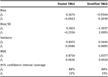
Section 5 compares the pooled TMLE described in this paper with alternative estimators for the parameters of longitudinal dynamic MSMs for survival. We provide a brief overview of the stratified TMLE [32], discuss scenarios in which each estimator may be expected to offer superior performance, and illustrate the breakdown of the stratified TMLE in a finite sample setting in which some interventions of interest have no support. As IPW estimators are currently the most common approach used to fit long-itudinal dynamic MSMs, we also discuss two IPW estimators for these parameters.
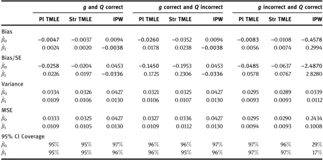
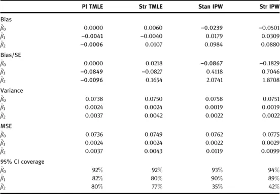
Section 6 presents a simulation study in which the pooled TMLE is implemented for a marginal structural working model for survival at timet. Its performance is compared to IPW estimators and to the stratified TMLE for a simple data generating process and in a simulation designed to be similar to the data analysis presented in the following section, which includes time-dependent confounding and right censoring.
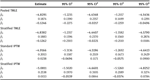
Section 7 presents the results of a data analysis investigating the effect of switching to second line therapy following immunologic failure of first line therapy using data from HIV-infected patients in the International Epidemiological Databases to Evaluate AIDS (IeDEA), Southern Africa. Throughout the paper, we illustrate notation and concepts using a simplified data structure based on this example.
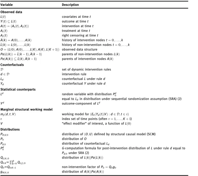
Appendices contain a derivation of the efficient influence curve, further simulation details, an alter-native TMLE, and reference table for notation. In online supplementary files, we present R code that implements the pooled TMLE, the stratified TMLE, and two IPW estimators for a marginal structural working model of survival. A corresponding publicly available R-package,ltmle, was released in May 2013 (http://cran.r-project.org/web/packages/ltmle/).
2 Definition of statistical estimation problem
Consider a longitudinal study in which the observed data structureO on a randomly sampled subject is coded as
O¼ðLð0Þ;Að0Þ;. . .;LðKÞ;AðKÞ;LðKþ1ÞÞ;
whereLð0Þare baseline covariates,AðtÞdenotes an intervention node at timet, andLðtÞdenotes covariates measured between intervention nodes Aðt1Þ and AðtÞ. Assume that there is an outcome process YðtÞ LðtÞ for t¼1;. . .;Kþ1, where LðKþ1Þ ¼YðKþ1Þ is the final outcome measured after the final treatment AðKÞ. The intervention node AðtÞ ¼ ðA1ðtÞ;A2ðtÞÞ has a treatment node A1ðtÞ and a censoring indicator A2ðtÞ, where A2ðtÞ ¼1 indicates that the subject is right censored by time t. We observe n
independent and identically distributed (i.i.d.) copiesO1;. . .;On ofO, and we will denote the probability
distribution of O with PO;0, or more simply, as P0. Throughout, we use subscript 0 to denote the true
distribution.
Running example. Here and in subsequent sections, we illustrate notation using an example in which
ni.i.d. HIV-infected subjects with immunological failure on first line therapy are sampled from some target population. Here t¼0 denotes time of immunological failure.LðtÞ denotes time-varying covariates, and includes CD4þT cell count at timetandYðtÞ, an indicator of death by timet. In addition to baseline values of these time-varying covariates, Lð0Þincludes non-time-varying covariates such as sex. The intervention nodes of interest areAðtÞ;t¼0;. . .K, whereAðtÞis defined as an indicator of switch to second line therapy by time t; in our simplified example, we assume no right censoring. For notational convenience, after a subject dies all variables for that subject are defined as equal to their last observed value.
2.1 Statistical model
We use the notation LðkÞ ¼ ðLð0Þ;. . .;LðkÞÞ to denote the history of time-dependent variable L from t¼0;. . .;k. Define the“parents”of a variableLðkÞ, denotedPaðLðkÞÞ, as those variables that precedeLðkÞ (i.e., PaðLðkÞÞ ¼Lðk1Þ;Aðk1Þ). Similarly, AðkÞ ¼ ðAð0Þ;. . .;AðkÞÞ is used to denote the history of the intervention process andPaðAðkÞÞto denote a specified subset of the variables that precedeAðkÞsuch that the distribution of AðkÞ given the whole past is equal to the distribution of AðkÞ given its parents (PaðAðkÞÞ LðkÞ;Aðk1Þ). Under our causal model, which we introduce below, these parent setsPaðLðkÞÞ andPaðAðkÞÞcorrespond to the set of variables that may affect the values taken byLðkÞandAðkÞ, respectively. We useQLðkÞ;0 to denote the conditional distribution ofLðkÞ, givenPaðLðkÞÞ, and, gAðkÞ;0 to denote the
conditional distribution ofAðkÞ, givenPaðAðkÞÞ. We also use the notation:g0:k;
Qk
j¼0gAðjÞ;0,g0;g0:K and
defineQ0:k;
Qk
j¼0QLðjÞ;0andQ0;Q0:Kþ1. In our example,QLðkÞ;0denotes the joint conditional distribution of
CD4 count and death at timek, given the observed past (including past CD4 count and switching history), and gAðkÞ;0denotes the conditional probability of having switched to second line by timekgiven the observed past
(deterministically equal to one for those time points at which a subject has already switched). The probability distributionP0ofOcan be factorized according to the time-ordering as
P0ðOÞ ¼Y Kþ1 k¼0 P0ðLðkÞjPa Lð ðkÞÞÞ YK k¼0 P0ðAðkÞjPa Að ðkÞÞÞ ¼YKþ1 k¼0 QLðkÞ;0ðOÞ YK k¼0 gAðkÞ;0ðOÞ ¼Q0ðOÞg0ðOÞ:
We consider a statistical modelMforP0that possibly assumes knowledge on the intervention mechanism
g0. For example, the treatment of interest, such as switch time, may be known to be randomized, or to be
assigned based on only a subset of the observed past. If Qis the set of all values forQ0and Gthe set of
possible values of g0, then this statistical model can be represented as M ¼ fP¼Q g:Q2 Q;g2 Gg. In
this statistical model,Qputs no restrictions on the conditional distributionsQLðkÞ;0,k¼0;. . .;Kþ1.
2.2 Causal model and counterfactuals of interest
By specifying a structural causal model [35, 36] or equivalently, a system of non-parametric structural equations, it is assumed that each component of the observed longitudinal data structure (e.g.AðkÞorLðkÞ)
is a function of a set of observed parent variables and an unmeasured exogenous error term. Specifically, consider the non-parametric structural equation model (NPSEM) defined by
LðkÞ ¼fLðkÞPa Lð ðkÞÞ;ULðkÞ; k¼0;. . .;Kþ1; and
AðkÞ ¼fAðkÞPa Að ðkÞÞ;UAðkÞ k¼0;. . .;K;
in terms of a set of deterministic functionsðfLðkÞ:k¼0;. . .;Kþ1Þ;ðfAðkÞ:k¼0;. . .;KÞ, and a vector of
unmeasured random errors or background factorsU¼ ðULð0Þ;. . .;ULðKþ1Þ;UAð0Þ;. . .;UAðKÞÞ[35, 36].
To continue our HIV example, we might specify a causal model in which both time-varying CD4 count, death, and the decision to switch potentially depended on a subject’s entire observed past, as well as unmeasured factors. Alternatively, if we knew that switching decisions were made only in response to a subject’s most recent CD4 count and baseline covariates, the parent set of AðkÞ could be restricted to exclude earlier CD4 count values.
This causal model represents a modelMF for the distribution ofðO;UÞand provides a parameterization of the distribution of the observed data structureO in terms of the distribution of the random variables
ðO;UÞ modeled by the system of structural equations. LetPO;U;0denote the latter distribution. The causal
modelMF encodes knowledge about the process, including both measured and unmeasured variables, that generated the observed data. It also implies a model for the distribution of counterfactual random variables under specific interventions on (or changes to) the observed data generating process. Specifically, a post-intervention (or counterfactual) distribution is defined as the distribution thatO would have had under a specified intervention to set the value of the intervention nodesA¼ ðAð0Þ;. . .;AðKÞÞ.
The intervention of interest might be static, with fAðkÞ;k¼0;. . .;K replaced by some constant for all subjects. For example, an intervention to setAðkÞ ¼0 fork¼0;. . .;K corresponds to a static intervention to delay switching indefinitely for all subjects. Alternatively, the intervention might be dynamic, with fAðkÞ;k¼0;. . .;K replaced by some specified function dkðLðkÞÞ of a subject’s observed covariates. For example, an intervention could set AðkÞ to 1 the first time a subject’s CD4 count drops below some threshold. As static regimes are a special case of dynamic regimes, in the following sections we define the statistical estimation problem and develop our estimator for the more general dynamic case. Throughout, we use“rule”to refer to a specific intervention, static or dynamic, that sets the values ofA.
Given a ruled, the counterfactual random variableLd¼ ðLð0Þ;Ldð1Þ;. . .;LdðKþ1ÞÞis defined by
deter-ministically setting all theAðkÞnodes equal todkðLðkÞÞin the system of structural equations. The probability distribution of this counterfactualLd is called the post-intervention or counterfactual distribution ofLand is
denoted withPd;0. Causal effects are defined as parameters of a collection of post-intervention distributions
under a specified set of rules. For example, we might compare mean counterfactual survival over time under a range of possible switch times.
2.3 Marginal structural working model
Our causal quantity of interest is defined using a marginal structural working model to summarize how the mean counterfactual outcome at timet varies as a function of the intervention ruled, time point t, and possibly some baseline covariate V that is a function of the collection of all baseline covariates Lð0Þ. Specifically, given a class of dynamic treatment rulesD, we can define a true time-dependent causal dose– response curve ðEPd;0ðYdðtÞjVÞ:d2 D;t2τÞ for some subsetτ f1;. . .;Kþ1g. Note that choice of V (as well as choice ofτandD) depends on the scientific question of interest. In many casesVwill be defined as the empty set. In other cases, it may be of interest to estimate how the causal dose–response curve varies depending on the value of some subset of baseline variables.
We specify a working modelΘ;fmβ:βgfor this true time-dependent causal dose–response curve. Our causal quantity of interest is then defined as a projection of the true causal dose–response curve onto this
working model, which yields a definitionmβ0 representing this projection. For example, ifYðtÞ 2 ½0;1, we may use a logistic working model Logitmβðd;t;VÞ ¼PJj¼1βjfjðd;t;VÞ for a set of basis functions, and define our causal quantity of interest as
ΨFðP O;U;0Þ ¼ argmin β E0 X t2τ X d2Dhðd;t;VÞ YdðtÞlogmβðd;t;VÞ ; þð1YdðtÞÞlogð1mβðd;t;VÞÞg;
wherehðd;t;vÞis a user-specified weight function. We discuss choice ofhðd;t;vÞfurther below. Such aΨF0¼β0solves the equation
0¼E0 X t2τ X d2Dhðd;t;VÞ d dβ0mβ0ðd;t;VÞ mβ0ð1mβ0Þ ðE0ðYdðtÞ jVÞ mβ0ðd;t;VÞÞ: This equation can be replaced by
0¼E0 X t2τ X d2Dhðd;t;VÞ d dβ0mβ0ðd;t;VÞ mβ0ð1mβ0Þ E0ðYdðtÞjLð0ÞÞ mβ0ðd;t;VÞ ; which corresponds with
ΨFðP O;U;0Þ ¼argmin β E0 X t2τ X t2Dhðd;t;VÞ E0ðYdðtÞjLð0ÞÞlogmβðd;t;VÞ þ ð1E0ðYdðtÞjLð0ÞÞÞlogð1mβðd;t;VÞÞ: In this case we have that
d dβ0mβ0ðd;t;VÞ
mβ0ð1mβ0Þ ¼ ðfjð
d;t;VÞ:j¼1;. . .;JÞ.
To be completely general, we will define our causal quantity of interest as a functionfofEðYdðtÞjLð0ÞÞ
acrossd2 D;t2τand the distributionQLð0Þ ofLð0Þ. Thus we define
ΨFðP
O;U;0Þ ¼f ðE0ðYdðtÞjLð0ÞÞ:d2 D;t2τÞ;QLð0Þ;0
:
In addition to including the above example, this general formulation allows us to include marginal structural working models on continuous outcomes and on the intervention-specific hazard.
2.3.1 Choice of a weight functionhðd;t;VÞ
Unless one is willing to assume that the MSM mβ is correctly specified, choice of the weight function changes the target quantity being estimated. Choice of the weight function should thus be guided by the motivating scientific question. For example, the simple weight functionhðd;t;VÞ ¼1 gives equal weight to all time points and switch times. Alternatively, choice of a weight function equal to the marginal probability of following ruledthrough timetwithin strata ofVgives greater weight to those rule, time, and baseline strata combinations with more support in the data, and zero weight to valuesðd;t;vÞwithout support. As discussed further below, choice of a weight function can thus also affect both identifiability of the target parameter and the asymptotic and finite sample properties of IPW and TML estimators.
2.3.2 Running example
Continuing our HIV example, recall that static regimes are a special case of dynamic regimes and define the set of treatment rules of interestDas the set of possible switch times (switch at time 0, switch at time 1,. . .,
never switch). We might focus on the marginal counterfactual survival curves under a range of switch times (withVdefined as the empty set). Alternatively, we might investigate how survival under a specific switch time differs among subjects that have a CD4þ T cell count <50 versus 50 cells/μl at time of failure (V¼IðCD4ð0Þ<50ÞwhereCD4ð0Þ Lð0Þ). For simplicity, for the remainder of the paper we use a running example in which we avoid conditioning on baseline covariates (i.e.V¼ fg).
The true time-dependent causal dose–response curveðE0ðYdðtÞÞ:d2 D;t21;. . .;Kþ1Þ corresponds to the set of counterfactual survival curves (through time Kþ1) that would have been observed for the population as a whole under each possible switch time. In this example, each ruledimplies a single vector
a; we usedðtÞto refer to the valueaðtÞimplied by ruledandsd to refer to the switch time assigned by rule
d. One might then specify the following marginal structural working model to summarize how the counter-factual probability of death by timetvaries as a function oftand assigned switch time:
Logitmβðd;tÞ ¼β0þβ1tþβ2ðdðt1ÞðtsdÞÞ;
wheredðt1ÞðtsdÞis time since switch for subjects who have switched by time t1, and otherwise 0. For simplicity, we choosehðd;tÞ ¼1 and define the target causal quantity of interest as the projection of
ðE0ðYdðtÞÞ:d2 D;t21;. . .;Kþ1Þontomβðd;tÞaccording to ΨFðP O;U;0Þ ¼argmin β E0 X t2τ X d2D YdðtÞlogmβðd;tÞ þð1YdðtÞÞlogð1mβðd;tÞÞ: ð1Þ
2.4 Identifiability and definition of statistical target parameter
We assume the sequential randomization assumption [11]
AðkÞaLdjPaðAðkÞÞ;k¼0;. . .;K ð2Þ (noting that weaker identifiability assumptions are also possible; see, for example, Robins and Hernan [9]). In our HIV example, the plausibility of this assumption would be strengthened by measuring all determinants of the decision to switch to second line therapy that also affect mortality via pathways other than switch time. We further assume positivity, informally an assumption of support for each rule of interest across covariate histories compatible with that rule of interest. Specifically, for eachd;t;Vfor whichhðd;t;VÞÞ0, we assume
P0ðAðkÞ ¼dkðLðkÞÞjLðkÞ;Aðk1Þ ¼dðLðk1ÞÞ>0;k¼0;. . .;K almost everywhere: ð3Þ In our HIV example, in whichhðd;tÞ¼1, a subject who has not already switched should have some positive probability of both switching and not switching regardless of his covariate history. Under these assump-tions, the counterfactual probability distribution ofLdis identified from the true observed data distribution
P0and given by theG-computation formulaP0d[11]:
P0dðlÞ ¼Y
Kþ1 k¼0
QdLðkÞ;0ðlðkÞÞ; ð4Þ
where Qd
LðkÞ;0ðlðkÞÞ ¼QLðkÞ;0ðlðkÞjlðk1Þ;Aðk1Þ ¼dðLðk1ÞÞ. Thus this G-computation formula P d 0 is
defined by the product over all LðkÞ-nodes of the conditional distribution of the LðkÞ-node, given its parents, and given Aðk1Þ ¼dðLðk1ÞÞ. If identifiability assumptions (2) and (3) hold for each rule d2 D, then the time-dependent causal dose–response curve ðE0ðYdðtÞjVÞ:d2 D;t2τÞ is also identified fromP0through the collection ofG-computation formulasðP0d:d2 DÞ. For the remainder of the paper, we
LetLd ¼ ðLð0Þ;Ldð1Þ;. . .;LdðKþ1ÞÞdenote a random variable with probability distributionPd 0, which
includes as a component the process Yd¼ ðYdð0Þ;Ydð1Þ;. . .;YdðKþ1ÞÞ. The above-defined causal
quan-tities can now be defined as a parameter of P0. For example, ifYðtÞ 2 ½0;1and the causal parameter of
interest is a vector of coefficients in a logistic MSM, then we have
ΨFðP O;U;0Þ ¼argmin β E0 X t X d2Dhðd;t;VÞ E0ðY dðtÞjLð0ÞÞlogm βðd;t;VÞ þð1E0ðYdðtÞjLð0ÞÞÞlogð1mβðd;t;VÞÞ ;ΨðP0Þ: The estimandψ0¼β0solves the equation
0¼E0 X t X d2Dhðd;t;VÞ d dβ0mβ0ðd;t;VÞ mβ0ð1mβ0Þ ðE0ðY dðtÞjLð0ÞÞ m β0ðd;t;VÞÞ:
The causal identifiability assumptions put no restrictions on the probability distribution P0 so that our
statistical model is unchanged, with the exception that we now also assume positivity (3). The statistical target parameter is now defined as a mappingΨ:M !IRJ that maps a probability distributionP2 MofO
into a vector of parameter valuesΨðPÞ.
The statistical estimation problem is now defined: We observeni.i.d. copiesO1;. . .;OnofO,P02 M
and we want to estimateΨðP0Þfor a defined target parameter mappingΨ:M !IRJ. For this estimation
problem, the causal model plays no further role – even when one does not believe any of the causal assumptions, one might still argue that the statistical parameterΨðP0Þ ¼ψ0represents an effect measure of interest controlling for all themeasuredconfounders.
3 Pooled TMLE of working MSM for dynamic treatments and
time-dependent outcome process
The TMLE algorithm starts out with defining the target parameter as aΨðQ;QLð0ÞÞfor a particular choiceQ that is easier to estimate than the whole likelihood Q. It requires the derivation of the efficient influence curve DðPÞ which can also be represented as DðQ;QLð0Þ;gÞ. Subsequently, it defines a loss function LðQ;QLð0ÞÞ for ðQ0;QLð0Þ;0Þ and a submodel ððQð;gÞ;QLð0Þð0Þ:; 0Þ through ðQ;QLð0ÞÞ at ð; 0Þ ¼0, indexed by the intervention mechanism g, chosen so that d
dð;0ÞLðQð;gÞ;QLð0Þð0ÞÞ
¼0 spans the efficient
influence curve DðQ;QLð0Þ;gÞ. Given these choices, it remains to define the updating algorithm which
simply uses the submodel through the initial estimator to determine the update by fitting ð; 0Þ with minimum loss based estimation (MLE), and this updating step is iterated till convergence at which point the MLE of ð; 0Þ equals 0. By the fact that an MLE solves its score equation, it then follows that the final update Qn;QLð0Þ;n also solves the efficient influence curve equation PiDðQn;QLð0Þ;n;gnÞðOiÞ ¼0, which
provides the foundation for its asymptotic linearity and efficiency. The remainder of this section presents each of these steps in detail.
An estimator ofψ0is efficient among the class of regular estimators if and only if it is asymptotically linear with influence curve DðQ0;g0Þ[37]. The efficient influence curve can thus be used as an ingredient
for the construction of an efficient estimator. One approach is to represent the efficient influence curve as an estimating functionDðQ;g;ψÞand define an estimatorψn as the solution ofPnDðQn;gn;ψÞ ¼0, given
initial estimators Qn;gn. This is referred to as the estimating equation methodology for construction of
maximum likelihood (substitution) estimator ΨðQnÞ that, as a by-product of the procedure, satisfies PnDðQn;gnÞ ¼0 and thus also solves the efficient influence curve estimating equation. Under
regularity conditions, one can now establish that, if DðQn;gnÞ consistently estimates DðQ0;g0Þ, then
ΨðQnÞ is asymptotically linear with influence curve equal to the efficent influence curve, so thatΨðQnÞ is asymptotically efficient. In addition, robustness properties of the efficient influence curve are naturally inherited by the TMLE.
Robins [13, 29] and Bang and Robins [22] reformulate the statistical target parameter and corresponding efficient influence curve for longitudinal MSMs on the intervention-specific mean as a series of iterated conditional expectations. For completeness, and to generalize to dynamic marginal structural working models possibly conditional on baseline covariates, as well as to general functions of the intervention-specific mean across a user-supplied class of interventions, we present this reformulation of the statistical target parameter below. The corresponding efficient influence curve is given in Appendix B. We will use the common notationPh¼ÐhðOÞdPðOÞfor the expectation of a functionhðOÞ with respect toP.
3.1 Reformulation of the statistical target parameter in terms of iteratively
defined conditional means
For the caseYdðtÞ 2 ½0;1in Section 2.4 we definedΨðPÞas
ΨðQÞ ¼argmin β E X t X d2Dhðd;t;VÞ Q d;t Lð1Þlogmβðd;t;VÞ þ ð1QLð1Þd;t Þlogð1mβðd;t;VÞÞ n o ; ð5Þ
where QdLð1Þ;t ¼EPðYdðtÞjLð0ÞÞ. Thus, ΨðPÞ only depends on P through Q
Lð1Þ¼ ðQdLð1Þ;t :d2 D;tÞ and QLð0Þ.
Therefore, we will also refer to the statistical target parameter ΨðPÞ as ΨðQÞ where we redefine Q;ðQLð1Þ;QLð0ÞÞ. For each given t, we can use the following recursive definition of EPðYdðtÞjLð0ÞÞ: for
k¼t;t1;. . .;1 we have QdLðkÞ;t ¼E YdðtÞjLdðk1Þ ¼ELðkÞ QdLðkþ1Þ;t jLðk1Þ;Aðk1Þ ¼dk1Lðk1Þ ;
where we defineQdLðtþ1Þ;t ¼YðtÞ. This definesQdLð1Þ;t as an iteratively defined conditional mean [22].
To obtainΨðQÞwe simply putQLð1Þ¼ ðQLð1Þd;t :d2 D;tÞ, combined with the marginal distribution ofLð0Þ
into the above representationΨðQÞ ¼ΨðQLð1Þ;QLð0ÞÞ. As mentioned in the previous section, we have that
ΨðQÞsolves the score equations given by
0¼EX t X d2Dhðd;t;VÞ d dβmβðd;t;VÞ mβð1mβÞ E Y dðtÞjLð0Þ mβðd;t;VÞ ;EX t X d2Dh1ðd;t;VÞ E Y dðtÞjLð0Þ mβðd;t;VÞ ; where we defined h1ðd;t;VÞ;hðd;t;VÞ d dβmβðd;t;VÞ mβð1mβÞ :
The TMLE for the linear working model using the squared error loss function is obtained by simply redefiningh1ðd;t;VÞ;hðd;t;VÞd
In general, the above shows that we can representΨðPÞ ¼fððEðYdðtÞjLð0ÞÞ:t;dÞ;Q
Lð0ÞÞas a function
fðQÞ, whereQ¼ ðQLð1Þ¼ ðEðYdðtÞjLð0Þ:d;tÞ;QLð0ÞÞand we have an explicit representation of the derivative
equation corresponding withf.
3.2 Estimation of intervention mechanism
g
0The log-likelihood loss function forg0is logg. Specifically, we can factorize the likelihoodg0as
g0¼ Q
K
k¼0
g1;kðA1ðkÞjPaðA1ðkÞÞÞg2;kðA2ðkÞjPaðA2ðkÞÞÞ;
whereðg1;k:kÞrepresents the treatment mechanism andðg2;k:kÞrepresents the censoring mechanism. Both
mechanisms can be estimated separately with a log-likelihood based logistic regression estimator, either according to parametric models, or preferably using the state of the art in machine learning. In particular, we can use the log-likelihood based super learner based on a library of candidate machine learning algorithms, which uses cross-validation to determine the best performing weighted combination of the candidate machine learning algorithms [39]. Use of such aggressive data-adaptive algorithms is recom-mended in order to ensure consistency ofgn.
If there are certain variables in thePaðAðkÞÞthat are known to be instrumental variables (variables that affect future Y nodes only via their effects on AðkÞ), then these variables should be excluded from our estimates ofg0in the TMLE procedure. In that case our estimate of the conditional distribution ofAðkÞis in
fact not estimating the conditional distribution ofAðkÞgiven its parents; however, for simplicity we do not make this explicit in our notation.
3.3 Loss functions and initial estimator of
Q
0We will alternate notation Qdk;t and QLðkÞd;t . Recall that ΨðQÞ depends on Q through QLð0Þ, and
Q;ðQdk;t :d2 D;t2τ;k¼1;. . .;tÞ. NoteQkd;t is a function oflðk1Þ,t¼1;. . .;Kþ1,k¼1;. . .;t, d2 D. We will use the following loss function forQdk;t:
Ld;t;k;Qd;t kþ1
ðQdk;tÞ ¼
IAðk1Þ ¼dk1ðLðk1ÞÞnQdkþ1;t logQdk;tþ1Qdkþ1;t log 1 Qdk;to:
This is an application of the log-likelihood loss function for the conditional mean of Qdkþ1;t given past covariates and given that past treatment has been assigned according to ruled. For example, fitting a parametric logistic regression model of Qkþ1d;t on past covariates among subjects with
Aðk1Þ ¼dk1ðLðk1ÞÞ would minimize the empirical mean of this loss function over the unknown parameters of the logistic regression model. Alternatively, one could use loss-based machine learning algorithms, such as loss-based super learning, with this loss function.
In this loss function, the outcomeQdkþ1;t is treated as known. In implementation of our estimator, it will be replaced by an estimate; we thus refer to Qdkþ1;t as a nuisance parameter in this loss function. The collection of loss functions fromk¼1;. . .;timplies a sequential regression procedure where one starts at k¼t and sequentially fits Qkd;t for k¼t;. . .;1. We describe this procedure in greater detail in the next subsection, for a sum-loss function that sums the above loss function over a collection of rules d2 D.
LQð QÞ;X t Xt k¼1 X d2DLd;t;k;Qdk;þt1ðQ d;t k Þ
for the wholeQ¼ ðQdk;t :d2 D;k¼1;. . .;t;t¼1;. . .;Kþ1Þ.
We will use the log-likelihood lossLðQLð0ÞÞ ¼ logQLð0Þas loss function for the distributionQ0;Lð0Þ of
Lð0Þ, but this loss will play no role since we will estimateQ0;Lð0Þ with the empirical distribution function
QLð0Þ;n. To conclude, we have presented a loss function for all components ofðQ;QLð0ÞÞour target parameter
depends on, and the sum-loss functionLQðQ;QLð0ÞÞ;LQðQÞ logQLð0Þis a valid loss function forðQ;QLð0ÞÞ
as a whole.
3.4 Non-targeted substitution estimator
These loss functions imply a sequential regression methodology for fitting each of the required components ofðQ;QLð0ÞÞ. These initial fits can then be used to construct a non-targeted plug-in estimator of the target parameterψ0. As noted, we estimate the marginal distribution ofLð0Þwith the empirical distribution. We now describe how to obtain an estimatorQdk;;nt,d2 D,k¼1;. . .;t, for any givent¼1;. . .;Kþ1. We define
Qtþ1d;t ¼YðtÞ for alld, and recall thatQdt;;ntis the regression of YðtÞ onAðt1Þ ¼dt1ðLðt1ÞÞandLðt1Þ. This latter regression can be carried out conditional on A1ðt1Þ;Lðt1Þ, stratifying only on not being censored through time t1 (i.e. A2ðt1Þ ¼0Þ). The resulting fit for all A1ðt1Þ values can then be evaluated at Aðt1Þ ¼dt1ðLðt1ÞÞ. In this manner, if certain rules have little support, one can still obtain an initial estimator that smoothes across all observations.
Given the regression fit Qdt;;nt, for a d2 D, we regress Qtd;;nt onto Aðt2Þ;Lðt2Þ and evaluate it at
Aðt2Þ ¼dt2ðLðt2ÞÞ, giving usQt1d;t;n. This is carried out for eachd2 D, giving usQt1d;t;nfor eachd2 D. Again, given this regression Qdt1;t;n, we regress this on Aðt3Þ;Lðt3Þ, and evaluate it at
Aðt3Þ ¼dt3ðLðt3ÞÞ, giving us Qt2d;t;n. We carry this out for each d2 D, giving us Qdt2;t;n, for each d2 D. This process is iterated until we obtain an estimator ofQd1;;ntðLð0ÞÞfor eachd2 D. Since this process is carried out for eacht¼1;. . .;Kþ1, this results in an estimatorQ1d;;nt for eachd2 Dandt¼1;. . .;Kþ1. We denote this estimator of Q1;0¼ ðQ1d;;0t :d;tÞ with Q1;n¼ ðQd1;;nt:d;tÞ. Note that a plug-in estimator
ΨðQ1;n;QLð0Þ;nÞofψ0¼ΨðQ1;0;QLð0ÞÞis now obtained by regressingQ1d;;nt ontod;t;Vaccording to the working
marginal structural model using weighted logistic regression based on the pooled sample
ðQd1;;ntðLið0ÞÞ;Vi;d;tÞ,d2 D;i¼1;. . .;n,t¼1;. . .;Kþ1, with weighthðd;t;ViÞ.
The pooled TMLE presented below utilizes this same sequential regression algorithm and makes use of these initial fits of Q0. In order to provide a consistent initial estimator of Q0 and thereby improve the
efficiency of the TMLE, use of an aggressive data-adaptive algorithm such as super learning [39] when generating the initial regression fits is recommended. These initial fits are then updated to remove bias in a series of targeting steps that rely on the fitgn ofg0. The updating steps involve submodels whose score
spans the efficient influence curve.
3.5 Loss function and least favorable submodel that span the efficient
influence curve
Recall that we use the notation g0:k¼
Qk
j¼0gAðjÞ for the cumulative product of conditional intervention
distributions. Consider the submodelQt
kð;gÞ¼ðQ d;t
LogitQdLðkÞ;t ð;gÞ ¼ LogitQLðkÞd;t þh1ðd;t;VÞ
g0:k1 ; k¼t;. . .;1:
This parameteris of same dimension asβandh1. This defines a submodelQtð;gÞwith parameterthrough
Qt¼ ðQd;t k :d2 D;k¼1;. . .;tÞ. Note that d dLd;t;k;Qdkþ;t1ðQ d;t k ð;gÞÞ ¼0 ¼h1ðd;t;VÞIðAðk1Þ ¼dk1ðLðk1ÞÞÞ g0:k1 ð Qdkþ1;t Qdk;tÞ:
This shows that d d XKþ1 t¼1 X d2D Xt k¼1Ld;t;k;Qd;t kþ1 ðQdk;tð;gÞÞj ¼0 ¼XKþ1t¼1 Xd2DXtk¼1h1ðd;t;VÞIðAðk1Þ ¼dk1ðLðk1ÞÞÞ g0:k1 ð Qdkþ1;t Qdk;tÞ ¼cðQÞ½DðPÞ DLð0ÞðQÞ
whereDðPÞis the efficient influence curve as presented in Corollary (1), Appendix (B), and we define cðQÞ;EQLð0Þ X t;dh1ðd;t;VÞ d dβmβðd;t;VÞ; giving DLð0ÞðQÞ ¼cðQÞ1X t;dh1ðd;t;VÞ Q d;t Lð1Þmβðd;t;VÞ : In other words, the sum-loss function
LQðQÞ ¼ XKþ1 t¼1 X d2D Xt k¼1Ld;t;k;Qdkþ;t1ðQ d;t k Þ
and submodel Qð;gÞ ¼ ðQkd;tð;gÞ:k;d;tÞ through Q¼ ðQkd;t:k;d;tÞ generates the component DðPÞ DLð0ÞðQÞof the efficient influence curveDðPÞ.
Consider also a submodelQLð0Þð0ÞofQLð0Þwith scoreDLð0ÞðQÞ, but this submodel and loss will play no
role in the TMLE algorithm since we will estimateQLð0Þwith its NPMLE, the empirical distribution ofLið0Þ, i¼1;. . .;n, so that the MLE of0will be equal to zero. This defines our submodelðQLð0Þð0Þ;Qð;gÞ:0; Þ.
The sum-loss function LQðQLð0Þ;QÞ ¼ LðQÞ logQLð0Þ and this submodel satisfy the condition that the
generalized score spans the efficient influence curve:
DðQ;gÞ 2 d dð; 0ÞLQ QLð0Þð0Þ;Qð;gÞ ð;0Þ¼0 * + : ð6Þ
3.6 Pooled TMLE
We now describe the TMLE algorithm based on the above choices of (1) the representation of ΨðPÞ as
ΨðQ; QLð0ÞÞ, (2) the loss function for ðQ; QLð0ÞÞ, and (3) the least favorable submodels ððQð;gÞ:Þ;ðQLð0Þð0Þ:0ÞÞ through ðQ;QLð0ÞÞ at ð; 0Þ ¼0 for fluctuating these parameters ðQ;QLð0ÞÞ. We utilize the same sequential regression approach described in Section 3.4, but now incorporate sequen-tial targeted updating of the inisequen-tial regression fits. We assume an estimatorgnofg0. We first specify where
Recall that we define Qdtþ1;t ¼YðtÞ for all d and that Qdt;;nt is the regression of YðtÞ on
Aðt1Þ ¼dt1ðLðt1ÞÞ;Lðt1Þ. For any given t¼1;. . .;Kþ1, the initial estimatorQdt;;nt is first updated toQdt;;nt;using a logistic regression fit of our least favorable submodels, as described below. For ad2 D, we then regress the updated regression fit Qtd;;nt; onto Aðt2Þ;Lðt2Þ, and evaluate it at
Aðt2Þ ¼dt2ðLðt2ÞÞ, giving us Qt1d;t;n. This is carried out for each d2 D, giving us Qdt1;t;n for each d2 D. The regressionsQdt1;t;nare then updated for eachd2 D, as described below, giving usQdt1;t;;nfor each d2 D. For ad2 D, we then regress the updated regression fitQdt1;t;;nonAðt3Þ;Lðt3Þand evaluate it at
Aðt3Þ ¼dt3ðLðt3Þ, giving usQt2d;t;n. We again carry this out for eachd2 D, giving usQdt2;t;n for each d2 Dand again update the resulting regressions, giving usQt2d;t;;n, for eachd2 D. This process is iterated until we obtain an updated estimatorQ1d;;nt;ðLð0ÞÞfor eachd2 D. Since this process is carried out for each t¼1;. . .;Kþ1, this results in an estimator Q1d;;nt; for each d2 D and t¼1;. . .;Kþ1. We denote this estimator ofQ1;0¼ ðQd1;;0t :d;tÞwithQ1;n¼ ðQ
d;t; 1;n :d;tÞ.
The updating steps are implemented as follows: for eacht2 f1;. . .;Kþ1g, and fork¼t tok¼1, we compute k;n;argmin k Pn X d2DLd;t;k;Qd;t; kþ1;n Qdk;;ntðk;gnÞ ;
and compute the corresponding updateQkd;;tn;¼Qdk;;tnðk;n;gnÞ, for alld2 D. Note that
k;n¼arg min X d2DLd;t;k;Qkdþ;t;1;nðQ d;t k;nð;gnÞÞ ¼arg min X d2D Xn
i¼1IðAiðk1Þ ¼dk1ðLiðk1ÞÞÞ
Qdkþ1;t;;nðLiðkÞÞlogQdk;;tnð;gnÞðLiðk1ÞÞ
n
þð1Qkþ1d;t;;nðLiðkÞÞÞlogð1Qdk;;ntð;gnÞðLiðk1ÞÞÞ
o
k¼1;. . .;Kþ1:
Thusk;n can be obtained by fitting a logistic regression of the outcomeQ d;t;
kþ1;nðLiðkÞÞwith offset Logit Q d;t k;n
on multivariate covariate
h1ðd;t;ViÞIðAiðk1Þ ¼dk1ðLiðk1ÞÞÞ=g0:k1ðOiÞ;
using a data set pooled acrossi¼1;. . .;n;d2 D(consisting ofn jDjobservations).
This defines the TMLE Qn¼ ðQkd;;nt;:d2 D;t;k¼1;. . .;tÞ. In particular,Q1;n¼ ðQ1d;;nt;:d2 D;tÞ is the TMLE ofQ1;0¼ ðE0ðYdðtÞjLð0ÞÞ:d2 D;tÞ. This defines now the TMLE ðQLð0Þ;n;QnÞ of ðQLð0Þ;0;Q0Þ, where
QLð0Þ;n is the empirical distribution ofLð0Þ.
The TMLE ofψ0 is the plug-in estimator corresponding withQ1;nand QLð0Þ;n: ψ
n¼ΨðQ1;n;QLð0Þ;nÞ:
This plug-in estimator ΨðQ1;n;QLð0Þ;nÞ of ψ0¼ΨðQ1;0;QLð0Þ;0Þ is obtained by regressing Qd1;;nt; onto d;t;V
according to the marginal structural working model in the pooled sample ðQd1;;nt;ðLið0ÞÞ;Vi;d;tÞ,
d2 D;i¼1;. . .;n,t¼1;. . .;Kþ1, using weightshðd;t;ViÞ.
An alternative pooled TMLE that only fits a single to compute the update is described in Appendix C.
3.7 Statistical inference for pooled TMLE
By construction, the TMLE solves the efficient influence curve equation 0¼PnDðQn;gn;ΨðQn;QLð0Þ;nÞÞ,
thereby making it a double robust locally efficient substitution estimator under regularity conditions, and positivity (3) (van der Laan [20], theorem 8.5, appendix A.18). Here, we provide standard error estimates and thereby confidence intervals for the case thatgn is a maximum likelihood estimator forg0using a correctly
specified semiparametric model forg0.
Specifically, ifgn is a maximum likelihood estimator ofg0according to a correctly specified
semipara-metric model forg0, andQnconverges to some possibly misspecifiedQ, then under regularity conditions the
TMLEψn is asymptotically linear with an influence curve given byDðQ;g0;ψ0Þ minus its projection onto
the tangent space of this semiparametric model for g0. As a consequence, the asymptotic variance of
ffiffiffi
n
p ðψ
nψ0Þ is more spread-out or equal to the covariance matrix 0¼P0DðQ;g0;ψ0Þ2. A consistent
estimator of this asymptotic variance is given by
n¼Pn DðQn;gn;ψnÞ 2 : As a consequence,ψnðjÞ 1:96 ffiffiffiffiffiffiffiffiffiffi nðj;jÞ p ffiffi n
p is an asymptotically conservative 95% confidence interval forψ0ðjÞ, and we can also use this multivariate normal limit result,ψn,Nðψ0;0=nÞ, to construct a simultaneous
confidence interval for ψ0 and to test null hypotheses about ψ0. This variance estimator treats weight functionhas known. Ifhis estimated, then this variance estimator still provides valid statistical inference for the statistical target parameter defined by the estimatedh.
In the case thatgn is a data-adaptive estimator converging tog0, we suggest (without proof), that this
variance estimator will still provide an asymptotically conservative confidence interval under regularity conditions. However, ideally the data-adaptive estimatorgn should also be targeted [40]. An approach to
valid inference in the case wheregn is inconsistent butQn is consistent is also discussed in van der Laan
[40]; however, it remains to be generalized to the parameters in this paper.
4 Implementation of the pooled TMLE
The previous section reformulated the statistical parameter in terms of iteratively defined conditional means and described a pooled TMLE for this representation. In this section, we illustrate notation and implemen-tation of this TMLE to estimate the parameters of a marginal structural working model on counterfactual survival over time.
4.1 The statistical estimation problem
We continue our motivating example, in which the goal is to learn the effect of switch time on survival. For illustration, focus on the two time point case where K¼1. Let the observed data consist ofni.i.d. copies O1;. . .;On ofOi¼ ðLið0Þ;Aið0Þ;Lið1Þ;Aið1Þ;Yið2ÞÞ,P0. LetLðtÞ ¼ ðYðtÞ;CD4ðtÞÞ, whereYðtÞ is an indicator
of death by timet, andCD4ðtÞis CD4 count at timet. Assume all subjects are alive at baseline (Yð0Þ ¼0). As above,AðtÞis an indicator of switch to second line by timet. We assume no right censoring so that all subjects are followed until death or the end of the study (for convenience define variable values after death as equal to their last observed value). We specify a NPSEM such that each variable may be a function of all variables that precede it and an independent error, and assume the corresponding non-parametric statis-tical model forP0.
Define the set of treatment rules of interestDas the set of all possible switch times f0;1;2g(where 2 corresponds to no switch). Each ruledimplies a single vectora¼ ðað0Þ;að1ÞÞ; we use dðtÞto refer to the
valueaðtÞimplied by ruled, andsdto refer to the switching time implied by ruled. We specify the following
marginal structural working model for counterfactual probability of death by timetunder ruled:
Logitmβðd;tÞ ¼β0þβ1tþβ2ðdðt1ÞðtsdÞÞ: ð7Þ
The target causal parameter is defined as the projection of ðE0ðYdðtÞÞ:d2 D;t2 f1;2gÞ onto mβðd;tÞ according to eq. (1).
Under the sequential randomization (2) and positivity (3) assumptions, EðYdðtÞjLð0ÞÞ ¼EðYdðtÞjLð0ÞÞ.
The target statistical parameter is defined as the projection ofðEðYdðtÞjLð0ÞÞ:d2 D;t2 f1;2gÞ, onto the
marginal structural working modelmβ, according to eq. (5) withhðd;tÞ ¼1.
4.1.1 Reformulation of the statistical target parameter Note that EðYdðt¼2ÞjLð0ÞÞ for rule d (denoted Qd;2
1 ) can be expressed in terms of iteratively defined
conditional means:
ELð1ÞEYð2ÞðYð2ÞjLð1Þ;Lð0Þ;Að1Þ ¼dð1Þ;Að0Þ ¼dð0ÞÞjLð0Þ;Að0Þ ¼dð0Þ; while EðYdðt¼1ÞjLð0ÞÞ (denoted Qd;1
1 ) equals EðYð1ÞjLð0Þ;Að0Þ ¼dð0ÞÞ. The statistical target parameter
ΨðQÞis defined by pluggingðQd1;1;Qd1;2Þ:d2 D, and the marginal distribution ofLð0Þinto eq. (5).
4.2 Estimator implementation
We begin by describing implementation of a simple plug-in estimator ofΨðQÞ.
4.2.1 Non-targeted substitution estimator
1. For each rule of interestd2 D, corresponding to each possible switch time, generate a vectorQd1;;n2 of lengthnfort¼2:
(a) Fit a logistic regression ofYð2Þ onLð1Þ;Lð0Þ;Að1Þ;Að0Þ and generate a predicted value for each subject by evaluating this regression fit atAð1Þ ¼dð1Þ;Að0Þ ¼dð0Þ. NoteE0ðYð2ÞjYð1Þ ¼1Þ ¼1, so the regression need only be fit and evaluated among subjects who remain alive at time 1. This gives a vectorQd2;;n2 of lengthn.
(b) Fit a logistic regression of the predicted values generated in the previous step on Lð0Þ;Að0Þ. Generate a new predicted value for each subject by evaluating this regression fit at Að0Þ ¼dð0Þ. This gives a vectorQd1;;n2 of lengthn.
2. For each rule of interestd2 Dgenerate a vectorQd1;;n1 of lengthnfort¼1: Fit a logistic regression of Yð1ÞonLð0Þ;Að0Þ and generate a predicted value for each subject by evaluating this regression fit at Að0Þ ¼dð0Þ.
3. The previous steps generatedQ1;n¼ ðQ1d;;nt;:d2 D;t2 f1;2gÞ. Stack these vectors to give a single vector
with length equal to the number of subjectsntimes the number of rulesj jD times the number of time pointsðn32Þ. Fit a pooled logistic regression ofQ1;n onðd;tÞ according to modelmβ (eq. 7), with
weights given byhðd;tÞ(here equal to 1). This gives an estimator of the target parameterΨðQÞ. We now describe how the pooled TMLE modifies this algorithm to update the initial estimatorQ1;n. In the
following section, we compare the pooled TMLE to this non-targeted substitution estimator and with other available estimators.
4.2.2 Pooled TMLE
1. EstimateP0ðAð1ÞjAð0Þ;Lð1Þ;Lð0ÞÞandP0ðAð0ÞjLð0ÞÞ. Denote these estimatorsg1;nandg0;n, respectively,
and letg0:1;n¼g0;ng1;n denote their product. In our example, this step involves estimating the
condi-tional probability of switching at time 0 given baseline CD4 count, and estimating the condicondi-tional probability of switching at time 1, given a subject did not switch at time 1, did not die at time 1, and CD4 count at times 0 and 1.
2. Generate a vectorQ2d;;n2;of lengthn Dj jfort¼2,k¼2:
(a) Fit a logistic regression ofYð2ÞonLð1Þ;Lð0Þ;Að1Þ;Að0Þ. Generate a predicted value for each subject and each d2 D by evaluating this regression fit at Að1Þ ¼dð1Þ;Að0Þ ¼dð0Þ. Note that E0ðYð2ÞjYð1Þ ¼1Þ ¼1, so the regression need only be fit and evaluated among subjects who remain alive at time 1. This gives a vector of initial valuesQd2;;n2 of lengthn Dj j.
(b) For each subject,i¼1;. . .;n, create a vector consisting of one copy ofYið2Þfor eachd2 D. Stack these copies to create a single vector of lengthn Dj j, denotedQd3;;n2;.
(c) For each subjecti¼1;. . .;nand eachd2 D, create a new multidimensional weighted covariate: hðd;t¼2Þ d dβmβðd;t¼2Þ mβð1mβÞ IðAi¼dÞ g0:1;nðOiÞ: In our example, hðd;tÞ ¼1, and
d dβmβðd;tÞ
mβð1mβÞ equals 1, t, anddðt1ÞðtsdÞ for the derivative taken
with respect toβ0;β1; andβ2, respectively. The following 33 matrix would thus be generated for each subjecti, with rows corresponding to switch at time 0, time 1, or do not switch:
1IðAið0Þ ¼1;Aið1Þ ¼1Þ g0:1;nðOiÞ 2IðAið0Þ ¼1;Aið1Þ ¼1Þ g0:1;nðOiÞ 2IðAið0Þ ¼1;Aið1Þ ¼1Þ g0:1;nðOiÞ 1IðAið0Þ ¼0;Aið1Þ ¼1Þ g0:1;nðOiÞ 2IðAið0Þ ¼0;Aið1Þ ¼1Þ g0:1;nðOiÞ 1IðAið0Þ ¼0;Aið1Þ ¼1Þ g0:1;nðOiÞ 1IðAið0Þ ¼0;Aið1Þ ¼0Þ g0:1;nðOiÞ 2IðAið0Þ ¼0;Aið1Þ ¼0Þ g0:1;nðOiÞ 0IðAið0Þ ¼0;Aið1Þ ¼0Þ g0:1;nðOiÞ 0 B B B B B B B B B B B B @ 1 C C C C C C C C C C C C A :
Stack these matrices to create a matrix withn Dj jrows and one column for each component ofβ (here, 3n3).
(d) Among those subjects still alive at the previous time point (Yð1Þ ¼0), fit a pooled logistic regres-sion ofQ3d;;n2;(theYð2Þvector) on the weighted covariates created in the previous step, suppressing the intercept and using as offset LogitQd2;;n2;, the logit of the initial predicted values for t¼2 and k¼2. This gives a fit for multivariate2. Denote this fit2;n¼ ðβ20;n;
β1
2;n; β2
2;nÞ.
(e) GenerateQd2;;n2;by evaluating the logistic regression fit in the previous step at eachd2 Damong those subjects for whomYð1Þ ¼0. For subjectiand ruled, evaluate
Expit
LogitðQ2d;;n2ðLi;dÞÞ þ
β0
2;n
g0;nðdð0ÞjLið0ÞÞg1;nðdð1ÞjLið0Þ;dð0Þ;Lið1ÞÞ
þ
β1
2;n2
g0;nðdð0ÞjLið0ÞÞg1;nðdð1ÞjLið0Þ;dð0Þ;Lið1ÞÞ
þ
β2
2;ndð1Þð2sdÞ
g0;nðdð0ÞjLið0ÞÞg1;nðdð1ÞjLið0Þ;dð0Þ;Lið1ÞÞ
:
3. Generate a vectorQ1d;;n2; of lengthn Dj jfort¼2,k¼1:
(a) Fit a logistic regression ofQd2;;n2;(generated in the previous step) onLð0Þ;Að0Þ. Generate a predicted value for each subject and eachd2 Dby evaluating this regression fit atAð0Þ ¼dð0Þ. This gives a vector of initial valuesQd1;;n2 of lengthn Dj j.
(b) For each subjecti¼1;. . .;nand eachd2 D, create the multidimensional weighted covariate as above, now fork¼1:
hðd;t¼2Þ d dβmβðd;t¼2Þ mβð1mβÞ IðAið0Þ ¼dð0ÞÞ g0;nðOiÞ :
The following 33 matrix would thus be generated for each subjecti, with rows corresponding to switch at time 0, time 1, or don’t switch:
1IðAið0Þ ¼1Þ g0;nðOiÞ 2IðAið0Þ ¼1Þ g0;nð;OiÞ 2IðAið0Þ ¼1Þ g0;nðOiÞ 1IðAið0Þ ¼0Þ g0;nðOiÞ 2IðAið0Þ ¼0Þ g0;nðOiÞ 1IðAið0Þ ¼0Þ g0;nðOiÞ 1IðAið0Þ ¼0Þ g0;nðOiÞ 2IðAið0Þ ¼0Þ g0;nðOiÞ 0IðAið0Þ ¼0Þ g0;nðOiÞ ; 0 B B B B B B B B @ 1 C C C C C C C C A :
Stack these matrices to create a matrix withn Dj jrows and one column for each dimension ofβ. (c) Fit a pooled logistic regression ofQd2;;n2; (the updated fit generated in step 2) on these weighted covariates, suppressing the intercept and using as offset LogitQd1;;n2;, the logit of the initial predicted values fort¼2 andk¼1. This gives a fit for multivariate1. Denote this fit1;n¼ ðβ1;0n; β1;1n; β1;2nÞ.
(d) Generate Qd1;;n2; by evaluating the logistic regression fit in the previous step at each d2 D. For subjectiand ruled, evaluate
Expit Logit Qd1;;n2ðLið0Þ;dð0ÞÞ
þ β0 1;n g0;nðdð0ÞjLið0ÞÞþ β1 1;n2 g0;nðdð0ÞjLið0ÞÞþ β2 1;ndð1Þð2sdÞ g0;nðdð0ÞjLið0ÞÞ ! : This gives an updated vectorQd1;;n2;of lengthn Dj j.
4. Generate a vectorQ1d;;n1;of lengthn Dj jfort¼1,k¼1:
(a) Fit a logistic regression ofYð1ÞonLð0Þ;Að0Þ. Generate a predicted value for each subject and each d2 Dby evaluating this regression fit atAð0Þ ¼dð0Þ. This gives a vector of initial valuesQd1;;n1 of lengthn Dj j.
(b) For each subject,i¼1;. . .;n, create a vector consisting of one copy ofYið1Þfor eachd2 D. Stack these copies to create a single vector of lengthn Dj j, denotedQd2;;n1;.
(c) For each subjecti¼1;. . .;nand eachd2 D, create a new multidimensional weighted covariate, fort¼1;k¼1: hðd;t¼1Þ d dβmβðd;t¼1Þ mβð1mβÞ IðAið0Þ ¼dð0ÞÞ g0;nðOiÞ :
The following 33 matrix would thus be generated for each subjecti, with rows corresponding to switch at time 0, time 1, or don’t switch:
1IðAið0Þ ¼1Þ g0;nðOiÞ 1IðAið0Þ ¼1Þ g0;nð;OiÞ 1IðAið0Þ ¼1Þ g0;nðOiÞ 1IðAið0Þ ¼0Þ g0;nðOiÞ 1IðAið0Þ ¼0Þ g0;nðOiÞ 0IðAið0Þ ¼0Þ g0;nðOiÞ 1IðAið0Þ ¼0Þ g0;nðOiÞ 1IðAið0Þ ¼0Þ g0;nðOiÞ 0IðAið0Þ ¼0Þ g0;nðOiÞ 0 B B B B B B B B @ 1 C C C C C C C C A :
Stack these matrices to create a matrix withn Dj jrows and one column for each component ofβ. (d) Fit a pooled logistic regression ofQ2d;;n1;(theYð1Þvector) on these weighted covariates, suppressing the intercept and using as offset LogitQd1;;n1;, the logit of the initial predicted values fort¼1 and k¼1. This gives a fit for multivariate1. Denote this fit1;n¼ ð1β;0n; β1;1n; β1;2nÞ.
(e) Generate Qd1;;n1; by evaluating the logistic regression fit in the previous step at each d2 D. For subjectiand ruled, evaluate
Expit LogitQd1;;n1ðLið0Þ;dð0ÞÞþ
β0 1;n g0;nðdð0ÞjLið0ÞÞþ β1 1;n g0;nðdð0ÞjLið0ÞÞþ β2 1;ndð0Þð1sdÞ g0;nðdð0ÞjLið0ÞÞ ! :
This gives an updated vectorQd1;;n1; of lengthn Dj j.
5. The previous steps generatedQ1;n¼ ðQd1;;nt;:d2 D;t¼1;2Þ. Stack these vectors to give a single vector with length equal to the number of subjectsntimes the number of rulesj jD times the number of time pointsðn32Þ. Fit a pooled logistic regression of Q1;n onðd;tÞ according model mβ (eq. 7), with weights given byhðd;tÞ(here equal to 1). This gives the pooled TMLE of the target parameterΨðQÞ.
5 Comparison with alternative estimators
In this section we compare the TMLE described with several alternative estimators available for dynamic MSMs for survival: non-targeted substitution estimators, IPW estimators, and the stratified TMLE of Schnitzer et al. [32].
5.1 Non-targeted substitution estimator
The consistency of non-targeted substitution estimators ofΨðQÞrelies entirely on consistent estimation of the Q portions of the observed data likelihood. For estimators based on the parametric G-formula this requires correctly specifying parametric estimators for the conditional distributions of all non-intervention nodes given their parents [7, 11, 12, 41]. For the non-targeted estimator described in Section (3.4), this requires consistently estimating the literately defined conditional meansQ;ðQdk;t: d2 D;t2τ;k¼1;. . .;tÞ. Correcta priorispecification of parametric models forQin either case is rarely possible, rendering such non-targeted plug-in estimators susceptible to bias. Further, while machine learning methods, such as Super Learning, can be used to estimateQnon-parametrically, the resulting plug-in estimator has no theory supporting its asymptotic linearity, and will generally be overly biased for the target parameterβ[21].
5.2 Inverse probability weighted estimators
The IPW estimator described in van der Laan and Petersen [2], Robins et al. [26] is commonly used to estimate the parameters of a dynamic MSM. In brief, this estimator is implemented by creating one data line for each subjecti, for eacht, and for eachdfor whichAðt1Þ ¼dðLðt1ÞÞ. Each data line consists ofYiðtÞ, any functions of ðd;t;ViÞ included as covariates in the MSM, and a weight hðdQ;t;ViÞIðAiðt1Þ¼dðLiðt1ÞÞÞ
t1
j¼0gnðAiðjÞjPaðAiðjÞÞÞ . A weighted logistic regression is then fit, pooling over time and rulesd.
The parameter mapping presented here for the TMLE suggests an alternative IPW estimator for dynamic MSM – namely, implement an IPW estimator for EðYdÞ (possibly within strata of V if V is discrete) for