Residual-based tests for cointegration and multiple deterministic structural breaks: A Monte Carlo study

(1)

Residual-based tests for cointegration and multiple

deterministic structural breaks: A Monte Carlo study

Matteo Mogliani

To cite this version:

Matteo Mogliani. Residual-based tests for cointegration and multiple deterministic structural

breaks: A Monte Carlo study. PSE Working Papers n2010-22. 2010. <halshs-00564897>

HAL Id: halshs-00564897

https://halshs.archives-ouvertes.fr/halshs-00564897

Submitted on 10 Feb 2011

HAL is a multi-disciplinary open access archive for the deposit and dissemination of sci-entific research documents, whether they are pub-lished or not. The documents may come from teaching and research institutions in France or abroad, or from public or private research centers.

L’archive ouverte pluridisciplinaire HAL, est destinée au dépôt et à la diffusion de documents scientifiques de niveau recherche, publiés ou non, émanant des établissements d’enseignement et de recherche fran¸cais ou étrangers, des laboratoires publics ou privés.

(2)

WORKING PAPER N° 2010 - 22

Residual-based tests for cointegration and

multiple deterministic structural breaks:

A Monte Carlo study

Matteo Mogliani

JEL Codes: C12, C13, C15, C22

Keywords: Cointegration, single-equation, structural

breaks, Monte Carlo simulations

P

ARIS

-

JOURDAN

S

CIENCES

E

CONOMIQUES

48,BD JOURDAN –E.N.S.–75014PARIS TÉL. :33(0)143136300 – FAX :33(0)143136310

www.pse.ens.fr

(3)

Residual-Based Tests for Cointegration and

Multiple Deterministic Structural Breaks:

A Monte Carlo Study

∗

Matteo Mogliani†

Paris School of Economics, France

First Version: November 11, 2009 This Version: August 31, 2010

Abstract

The aim of this paper is to study the performance of residual-based tests for cointegra-tion in the presence of multiple deterministic structural breaks via Monte Carlo simulacointegra-tions. We consider the KPSS-type LM tests proposed in Carrion-i-Silvestre and Sans`o (2006) and in Bartley, Lee, and Strazicich (2001), as well as the Schmidt and Phillips-type LM tests proposed in Westerlund and Edgerton (2007). This exercise allow us to cover a wide set of single-equation cointegration estimators. Monte Carlo experiments reveal a trade-off be-tween size and power distortions across tests and models. KPSS-type tests display large size distortions under multiple breaks scenarios, while Schmidt and Phillips-type tests ap-pear well-sized across all simulations. However, when regressors are endogenous, the former group of tests displays quite high power against the alternative hypothesis, while the latter shows severe low power.

Keywords: Cointegration; single-equation; structural breaks; Monte Carlo simulations.

JEL classification: C12, C13, C15, C22.

∗

The author is indebted to Giovanni Urga and Eduardo Rossi for helpful comments and discussions. He also wish to thank participants in the CEA reading group seminar at Cass Business School for useful discussions. However, the usual disclaimer applies.

†

Corresponding address: Paris School of Economics, Paris-Jourdan Sciences Economiques, 48 Boulevard Jour-dan, 75014 Paris (France). Tel: +33 (0)1 43 13 63 22. Fax: +33 (0)1 43 13 63 10. Email: [email protected].

(4)

1 Introduction

Cointegration has been at the heart of a vast macroeconomic and econometric research since the

seminal contribution of Engle and Granger (1987). This concept,i.e., the hypothesis that one

stationary linear combination of individually non-stationary variables exists, has been widely used for empirical purposes in many areas of economics. Indeed, the development of cointe-grating and error-correction models allowed applied economists to shed light on long-run and short-run theoretical economic relationships, such as, for instances, money demand (e.g., Hendry and Ericsson, 1991, and Stock and Watson, 1993), balanced growth (e.g., King et al., 1991) and purchase power parity (e.g., Taylor and McMahon, 1988, and Cheung and Lai, 1993).

Many cointegration tests have been proposed in the econometric literature. Among them, the class of residual-based tests is the most popular, thanks to the simple computation and the straight interpretation in terms of economic theory. Following the unit-root testing approach, the literature has proposed tests for the null hypothesis of non-cointegration (Engle and Granger, 1987; Phillips and Ouliaris, 1990), as well as tests for the null hypothesis of cointegration (Hansen, 1992; Shin, 1994).

These tests show nevertheless serious size distortions when specific features of data are neglected. Indeed, one potential feature of long-run economic relationships is structural breaks,

i.e., the significant change of one or more parameters affecting persistently the data generating

process (DGP) of the underlying economic model. This issue is addressed in Gregory and Hansen (1996), who extend the general framework of Engle and Granger (1987) and Phillips and Ouliaris (1990) to account for the presence of one structural break. However, as pointed out

in Carrion-i-Silvestre and Sans`o (2006), the statistical tests proposed in Gregory and Hansen

(1996) are not able to discern between the situation of unstable cointegrating relationship and that of stability with regime-shifts, the null hypothesis of non-cointegration being tested against the alternative of cointegration with break.

Residual-based tests recently proposed in the literature address this issue through the inclu-sion of structural breaks under both the null and the alternative hypothesis. The generalization of the break hypothesis makes the latter tests independent (stand alone tests for the hypothe-sis of cointegration or non-cointegration), compared to the complementarity role of the former (auxiliary tests for the hypothesis of spurious cointegration led by a neglected break). However,

(5)

these recent contributions have only explored the “one structural break” hypothesis. This is mainly due to the well-known econometric circular problem of, on the one hand, estimating and testing for multiple (deterministic or stochastic) breaks in the presence of non-stationary variables (unit-root) or cointegrated systems, and, on the other hand, assessing non-stationarity or cointegration when breaks are neglected or their actual number is misspecified. This issue has then attracted increasing attention in the econometric literature during the last decade. To deal with the circular problem in the unit-root testing, various approaches have been re-cently proposed to check for the presence of breaks (in trend and level) in univariate I(1) or I(0) processes (Perron and Zhu, 2005; Harvey et al., 2009a,b; Perron and Yabu, 2009; Kejriwal and Perron, 2009a), as well as to embed the hypothesis of multiple breaks in a large class of standard unit-root tests (Carrion-i-Silvestre et al., 2009). Based on these theoretical develop-ments, Kejriwal and Lopez (2010) propose a sequential testing strategy designed to help applied economists to minimize the model specification error.

As to the circular problem in the cointegration testing, more emphasis has been put on the selection of the actual number of breaks in long-run regressions. To tackle this issue in a single-equation cointegration framework, approaches based on global minimizers algorithms (Bai and Perron, 1998, 2003; Qu, 2007; Kejriwal and Perron, 2009b), as well as sequential bootstrap procedures (De Peretti and Urga, 2004), have been so far proposed in the literature. Indeed, as pointed out by Mogliani, Urga, and Winograd (2009), accounting for multiple breaks in economic relationships can be a crucial issue when dealing, for instances, with emerging economies and/or long span datasets. However, to our knowledge, too little has been said in the literature about the behaviour of residual-based tests for cointegration when multiple breaks affect the long-run relationship of non-stationary series.

The main aim of this paper is to compare the size and power distortions of residual-based tests for cointegration in the case of multiple breaks. For this purpose, we run Monte Carlo simulations involving several single-equation cointegration estimators (OLS, DOLS, DGLS, FM-OLS and CCR) and breaks scenarios. For the latter issue, we follow Perron (1989, 1990) and Hao (1996) and we only consider deterministic structural breaks (constant and trend). We also account for endogenous regressors and potential misspecification of model residuals. The results of the study should lead to specific recommendations for applied economists in terms of the best

(6)

performing estimator/test pair to use for cointegrating regression models with multiple breaks. We consider the residual-based tests for the null hypothesis of cointegration proposed in

Bartley, Lee, and Strazicich (2001) and Carrion-i-Silvestre and Sans`o (2006). These

contribu-tions deal with the generalization of the univariate LM test of Kwiatkowski, Phillips, Schmidt, and Shin (1992) - henceforth KPSS -, as in Shin (1994), Hao (1996) and Lee (1999), to the case of cointegration with one structural break, while efficient estimates of the cointegrating relation-ship are carried out through the Canonical Cointegration Regression (Park, 1992), the dynamic OLS (Saikkonen, 1991; Stock and Watson, 1993) and the Fully-Modified approach (Phillips and Hansen, 1990). We also consider testing procedures proposed in Westerlund and Edgerton (2007) and involving instead the null hypothesis of non-cointegration. This work extends the univariate LM test of Schmidt and Phillips (1992) - henceforth SP - to the cointegration with a single break framework. The proposed statistical tests are built upon the OLS estimate of the cointegrating relationship (Engle and Granger, 1987; Phillips and Ouliaris, 1990), and they are thus mainly designed for strictly exogenous regressors.

Our main findings show that KPSS-based tests display severe size distortions when more deterministic breaks are included in the cointegration model, in particular when both level and trend breaks are considered. The opposite is true for the tests proposed in Westerlund and Edgerton (2007), which appear quite correctly sized across all our simulation exercises. However, these results are reverted in the power analysis: KPSS-based tests show quite high power against the alternative hypothesis in all simulations, while SP-based tests show very low power which tends to be close to the nominal size. Simulations reveal that the latter result is mainly driven by the presence of endogenous regressors. Overall, tests based on the DOLS and, in particular, on the DGLS estimators display the best size-power performance.

The remainder of the paper is as follows. In Section 2, we introduce a general model of cointegration with structural breaks and we briefly describe the estimators and the residual-based tests of cointegration studied in this paper. In Section 3 we define the DGP used for simulation purposes and we explain the Monte Carlo design. In Section 4 we discuss simulation results. Section 5 concludes.

(7)

2 Estimators and Tests for Cointegration with Structural Breaks

In this Section we briefly describe the general single-equation cointegration model with struc-tural breaks and six alternative residual-based tests for cointegration used in our Monte Carlo

experiments. Four of these test statistics (CS_DOLS, CS_DGLS, CS_FM and BLS_CCR) are based

on the null hypothesis of cointegration (Bartley, Lee, and Strazicich, 2001; Carrion-i-Silvestre

and Sans`o, 2006), while the remaining two (W E_Φ and W E_t_-stat) are based on the null of

non-cointegration (Westerlund and Edgerton, 2007). For ease of exposition, statistical tests are presented along with their related estimators of cointegrating relationships.

2.1 The Cointegrated Regression Model

Let’s assume that the data generating process (DGP) is of the form:

yt=α+g(t) +x0tβ+et, (1)

with

et= ρet−1+εt xt= xt−1+µt,

wheret= 1, . . . , T is the time series index,xtis theK-dimensional vector of I(1) regressors and

εtandµtare i.i.d. processes with distributionN(0,Σ). We defineg(t) as the function collecting

the deterministic components of the model, except for the constant. Following Perron (1989,

1990), Hao (1996), Bartley, Lee, and Strazicich (2001) and Carrion-i-Silvestre and Sans`o (2006),

we choose to study an empirically relevant set of deterministic functions:

g(t) =            θ1DUt Model A τ t+θ1DUt Model B τ t+θ1DUt+θ2DTt Model C (2)

(8)

whereDUt= (DU1,t, . . . , DUm,t)0andDTt= (DT1,t, . . . , DTm,t)0are the vectors of deterministic breaks and DUj,t =      1, fort > Tjb 0, otherwise and DTj,t =      (t−Tjb), fort > Tjb 0, otherwise

is the structure of deterministic breaks at dates Tjb =λjT, with λj ∈ (0,1), for j = 1, . . . , m,

where m is the number of breaks. Model A allows for multiple level breaks without a linear

trend. Model B allows for a linear trend and multiple level breaks. Finally, Model C allows for both multiple level and trend breaks, which are assumed for simplicity to pairwise occur at the same date.

2.2 A Test Based on the OLS Estimator

A test based on the standard OLS estimator of the cointegrating relationship in (1) (Engle and Granger, 1987; Phillips and Ouliaris, 1990) is proposed in Westerlund and Edgerton (2007) -henceforth WE. Following Schmidt and Phillips (1992), WE propose an LM-type test for the null hypothesis of non-cointegration against the alternative of cointegration, with a structural break under both the null and the alternative.

According to the LM (score) principle, the cointegration test is obtained from the following regression:

∆ ˆSt=ϑ+ Φ ˆSt−1+t, (3)

where ϑ is a constant, t is the error term, ˆSt = yt−αˆ−gˆi(t)−x0tβˆ and ˆα is the restricted

maximum likelihood estimate of ˜α=α+e0, given by ˆα=y1−ˆgi(1)−x01βˆ. Estimates of ˆβ and

parameters in ˆgi(t), fori={A, B, C}, are obtained from the OLS regression of ∆ytover ∆gi(t)

and ∆x0_t. It is worth noticing that the expression ∆gi(t) involves one-period jumps (∆DUt) and

changes in drift (∆DTt), rather than constant (DUt) and trend (DTt) breaks. From Equation

(3), the hypothesis of non-cointegration can be formulated as a test of Φ = 0 against Φ < 0,

(9)

the following two statistical tests: W E_Φ=T ×Φˆ and W E_t_-stat = ˆ Φ ˆ σ × v u u t T X t=2 ( ˆSt−1)2p, (4)

where ˆσ is the estimated standard error from regression (3) and ( ˆSt−1)p is the error from

projecting ˆSt−1 onto its mean value. To account for autocorrelated and heteroskedastic errors,

WE follow the parametric correction proposed in Ahn (1993) and include augmented terms in Equation (3) : ∆ ˆSt=ϑ+ Φ ˆSt−1+ p X j=1 ψj∆ ˆSt−j+t, (5)

where the optimal lag orderpis chosen by following the “general to specific” procedure suggested

by Perron (1989), Campbell and Perron (1991) and Ng and Perron (1995). In our Monte Carlo

simulations we allow for a maximum number of 6 lags.1 _{WE show that only the statistic}_{W E}

Φ

is affected by the presence of autocorrelated errors. This requires the following correction:

W E_Φ=T ×Φˆ × r ˆ ω ˆ σ2, (6)

where ˆσ2 is the residual variance from the augmented test regression (5) and ˆω is the long-run

variance of ∆ ˆSt evaluated at frequency zero:

ˆ ω= 1 T T X t=1 ∆ ˆSt∆ ˆS_t0+ 2 T T X j=0 w j M T X t=j+1 ∆ ˆSt∆ ˆS_t0−j,

wherew(·) andM are the kernel function and the bandwidth parameter, respectively. We follow

WE and we use a Bartlett kernel with bandwidth parameter M =p (the optimal lag order in

the auxiliary regression (5)).

For the case of Model B, it can be shown that both W EΦ and W Et-stat statistics follow

the asymptotic distributions derived in Schmidt and Phillips (1992). In addition, distributions

are unaffected by the presence of multiple mean breaks, the number of regressors (K) and the

breaks fraction (λj). For the case of Model A, our simulations show that the exclusion of the

1

We sequentially test at 5% level the significance of the last term in the augmented test regression (5), until either the optimal lag is found orp= 0.

(10)

linear trend from the cointegrating equation does affect the asymptotic distribution of both statistics. Nevertheless, distributions are unaltered by the presence of multiple mean breaks. Differently, for the case of Model C, our simulations show that the statistics under consideration follow asymptotic distributions which depend on the number of breaks and their location in the

sample (λj).

It is worth noticing that the testing procedure proposed in WE is valid until regressors xt

are strictly exogenous. Relaxing this assumption would imply a potential bias arising from the

OLS estimate of ˆβ for the computation of ˆSt. To correct for endogeneity bias, WE propose

to estimate ˆβ by IV. In practice, finding out consistent instruments for endogenous regressors

can be difficult in the context of cointegrated macroeconomic time series. For this reason,

in our simulations we prefer studying the performance of W EΦ and W Et-stat statistics under

endogeneity bias.

2.3 A Test Based on the Dynamic Leads-and-Lags Estimator

A test based on the leads-and-lags correction of the cointegrating regression (Saikkonen, 1991;

Stock and Watson, 1993) is developed in Carrion-i-Silvestre and Sans`o (2006) - henceforth

CS. Following Shin (1994), CS propose a LM-type test for the null hypothesis of cointegration against the alternative of non-cointegration, with a structural break under both the null and the

alternative. Let’s definevt= ∆xtand ηt= (et, v0_t) and assume thatηt satisfies the multivariate

invariance principle (Herrndorf, 1984; Phillips and Durlauf, 1986):

T−1/2Ω

[T r] X

t=1

ηt⇒W(r), 0≤r≤1,

where ⇒ denotes weak convergence in probability and W(r) = (W1(r), W2K(r)0)0 is a (K

+1)-dimensional Wiener process. Ω is the long-run covariance matrix, which can be written

(parti-tioned in conformity with ηt) as:

Ω = lim T→∞ 1 T T X t=1 T X j=1 E(ηjηt0) =    ω11 ω12 ω12 Ω22   = Σ + Λ + Λ 0_,

(11)

where long-run variances ω11 and Ω22 of processes W1(r) and W2K(r) are positive definite to

rule out multicointegration (Granger and Lee, 1990) and

Σ = lim T→∞ 1 T T X t=1 E(ηtη_t0) =    σ11 σ12 σ12 Σ22    Λ = lim T→∞ 1 T T X t=1 t X j=1 E(ηjη0_t) =    λ11 λ12 λ12 Λ22   .

Standard asymptotics cannot apply here because of the presence of correlation between

disturbance terms. This means that regressors xt are not strictly exogenous and the OLS

estimator of the cointegrating regression (1) is inefficient. To overcome this problem, CS propose to estimate (1) through the following Dynamic OLS regression:

yt=α0+gi(t) +x0tβ+ k X j=−k ∆x0_t−jξj +e ∗ t, (7)

where k is the (finite truncated) number of leads and lags for first-differenced non-stationary

regressors.

Since errors e∗_t can be serially correlated and uncorrelated with the regressors at all leads

and lags, we follow Stock and Watson (1993) and we introduce the Dynamic GLS estimator. A

feasible DGLS estimator is constructed by transforming regressors in (7) as ˜xt=x0_tϕˆ(L), where

ˆ

ϕ(L) is an estimate of the lag polynomial of residuals ϕ(L).2

In our Monte Carlo experiments, we construct ϕ(L) as an AR(1) model of residuals. We

follow the Cochrane-Orcutt iterative procedure and we allow the AR(1) parameter to converge across the sequential estimation. Finally, we allow the number of leads and lags to be selected

by the SBC criterion, starting with a maximum number of 4.3

The multivariate LM-type test proposed in CS is then given by:

CS_DOLS= T −2 ˆ ω₁₁∗ _·₂ × T X t=1 (S_t∗)2 and CS_DGLS= T −2 ˆ ω₁₁∗ _·₂ × T X t=1 (S_t∗)2, (8) 2

It is worth noticing that the DGLS estimator is not considered in the original work of CS, but it is expressly introduced by the author of the present paper.

3

The use of this information criterion is supported by simulation results reported in Kejriwal and Perron (2008).

(12)

where S_t∗ =Pt

j=1eˆ∗j, ˆe∗t are estimated residuals from DOLS/DGLS regression (7) and ˆω∗11·2 is

any consistent estimate of ω₁₁_·₂ = ω₁₁−ω₁₂Ω−₂₂1ω₂₁, i.e., the endogeneity-corrected long-run

variance of residualset. In practice, a consistent estimate of ω₁₁_·₂ can be obtained as follows:

ˆ ω₁₁∗ ·2 = 1 T T X t=1 ˆ e∗_teˆ∗0_t + 2 T T X j=0 w j M T X t=j+1 ˆ e∗_teˆ∗0_t−j,

withw(·) andM being the kernel function and the bandwidth parameter, respectively. To avoid

the inconsistency on the estimate of the long-run variance ˆω₁₁∗ _·₂, we follow CS and we use the

kernel and the bandwidth parameter proposed in Kurozumi (2002). This issue will be discussed in Section 3.3.

For the case of a single break, CS show that the asymptotic distribution of the test statistic

depends on the number of regressors (K), the break fraction (λ) and the deterministic model

considered (gi(t)). This result can be readily generalized to the case of multiple structural

breaks. In this case, the number of breaks (m) and their location in the sample (λj) also affect

the asymptotic distribution.

2.4 A Test Based on the Fully-Modified Estimator

Carrion-i-Silvestre and Sans`o (2006) also extend the test presented above to the Fully-Modified

estimator of cointegrating relationships (Phillips and Hansen, 1990),i.e., solving non-parametrically

the issue of the OLS inefficiency when regressors are non-strictly exogenous.

Consider the set of asymptotic assumptions illustrated in the first part of paragraph 2.3.

We exploit here the long-run correlation properties of the innovations vector ηt = (et, v0t) to

rule out the bias due to the endogeneity of regressors xt. Preliminary simulations suggest that

cointegration tests based on the pre-whitened Fully-Modified estimator lead to improved results in terms of size and power. We then follow Andrews and Monahan (1992) and Hansen (1992)

and we build the Fully-Modified correction by firstly fitting a VAR(1) toηtand then consistently

estimating the long-run covariance matrix from whitened residuals ˆεt= ˆηt−ηˆ0_t₋₁ζˆ:

Ωε= 1 T T X t=1 ˆ εtεˆ0_t+ 2 T T X j=0 w j M T X t=j+1 ˆ εtεˆ0_t−j,

(13)

with partitions Σε = 1 T T X t=1 ˆ εtεˆ0_t Λε = 1 T T X j=0 w j M T X t=j+1 ˆ εtεˆ0t−j,

where the kernel function w(·) used for our simulations is the Quadratic Spectral and its

associated plug-in bandwidth estimator (Andrews, 1991).4 The long-run covariance matrix

used for the Fully-Modified estimation is then recolored: Ω = (I − ζˆ)−1Ωε(I −ζˆ0)−1 and

Λ = (I−ζˆ)−1Λε(I−ζˆ0)−1−(I−ζˆ)−1ζˆΣ, where Σ = 1/TPT_t ηtˆηˆ0t.

Fully-Modified estimation is then computed by partitioning Ω and Λ, setting ω₁₁_·₂ =ω₁₁−

ω₁₂Ω−₂₂1ω₂₁ and λ+₂₁ = λ₂₁−Λ₂₂Ω−₂₂1ω₂₁ and transforming the dependent variable y_t+ = y_t−

ω₁₂Ω−₂₂1v_t0. The Fully-Modified estimator of cointegrating parameters is obtained through the

following OLS regression:

β_X+ = (X_t0Xt)−1 X_t0y_t+−κλ+₂₁,

whereXtis the vector of regressors (deterministic and stochastic) included in (1) andκ= [0, I]

is a matrix of dimension (d+K)×K, with first d×K zero elements followed by a K ×K

identity matrix (dbeing the number of deterministic regressors in the model).

Fully-Modified residuals ˆe+_t =y+_t −X_t0βˆ_X+ are then used to compute the LM-type statistic:

CS_FM= T −2 ˆ ω₁₁+_·₂ × T X t=1 S_t+2, (9) where S_t+ = Pt j=1eˆ +

j and the consistent estimate of the long-run variance of residuals e

+ t is obtained as follows: ˆ ω₁₁+_·₂ = 1 T T X t=1 ˆ e+_t eˆ+_t0+ 2 T T X j=0 w j M T X t=j+1 ˆ e+_t ˆe+_t₋0_j, 4

The Quadratic Spectral kernel is defined asw(x) = 25 12π2_x2

sin(6πx/5)

(6πx/5) −cos(6πx/5)

and its optimal band-width parameter is M = 1.3221( ˆα(2)T)1/5, where ˆα(2) = Pp

a=1 4ρ2_aσ_a2 (1−ρa)8 . Pp a=1 σ2_a (1−ρa)4 is obtained from an

(14)

withw(·) andM being, respectively, the kernel function and the bandwidth parameter proposed in Kurozumi (2002) (see Section 3.3).

For the case of a single break, CS show that the asymptotic distribution of the test statistic

based on the Fully-Modified correction is the same as assuming xt strictly exogenous. Again,

the asymptotic distribution depends on the number of regressors (K), the break fraction (λ)

and the deterministic structure (gi(t)). In the multiple breaks framework considered here, the

asymptotic distribution also depends on the number of breaks (m) and their location in the

sample (λj).

2.5 A Test Based on the Canonical Cointegration Estimator

A test based on thefeasibleCanonical Cointegration Regression estimator (Park, 1992) is

devel-oped in Bartley, Lee, and Strazicich (2001) - henceforth BLS. The authors propose a LM-type test for the null hypothesis of cointegration against the alternative of non-cointegration, with a structural break under both the null and the alternative.

As for the Fully-Modified estimator, preliminary simulations suggest that tests based on the pre-whitened CCR estimator lead to improved results in terms of size and power. We then fit

a VAR(1) to ηt and we compute consistent estimate of the long-run covariance matrix from

whitened residuals ˆεt= ˆηt−ηˆ0_t−1ζˆ: Ωε= 1 T T X t=1 ˆ εtεˆ0_t+ 2 T T X j=0 w j M T X t=j+1 ˆ εtεˆ0_t−j, with partitions Σε = 1 T T X t=1 ˆ εtεˆ0t Λε = 1 T T X j=0 w j M T X t=j+1 ˆ εtεˆ0_t−j Γε = 1 T T X t=1 ˆ εtεˆ0_t+ 1 T T X j=0 w j M T X t=j+1 ˆ εtεˆ0_t−j,

where the kernel functionw(·) used for our simulations is the Quadratic Spectral and its

(15)

Ωε= Σε+ Λε+ Λ0ε= Γε+ Λ0ε. The long-run covariance matrix used for the CCR estimation is

then recolored: Ω = (I−ζˆ)−1Ωε(I−ζˆ0)−1 and Λ = (I−ζˆ)−1Λε(I−ζˆ0)−1−(I−ζˆ)−1ζˆΣ, where

Σ = 1/TPT

t ηtˆηˆ 0 t.

CCR estimation is computed by first transforming the regressand and the stochastic regres-sors and then estimating by OLS the following corrected cointegration model:

y_t?=α0+gi(t) +x?t0β?+e?t, (10)

wherey_t? =yt−(Σ−1Γ₂βˆ+ (0, ω₁₂Ω−₂₂1)0)0ηtˆ,x_t? =xt−(Σ−1Γ₂)0ηtˆ, Γ₂ = (γ₁₂,Γ₂₂) and ˆβ is the vector of estimated parameters obtained from the auxiliary regression of the uncorrected model (1).

CCR residuals ˆe?_t =y_t?−αˆ0−gi(t)−x?t0βˆ? are then used to compute the LM-type statistic:

BLS_CCR= T −2 ˆ ω?₁₁_·₂ × T X t=1 S_t+2, (11) where S_t+ = Pt

j=1eˆ?j and the consistent estimate of the long-run variance of residuals e?t is

obtained as follows: ˆ ω₁₁? _·₂ = 1 T T X t=1 ˆ e?_teˆ?_t0+ 2 T T X j=0 w j M T X t=j+1 ˆ e?_teˆ?_t₋0_j,

withw(·) andM being, respectively, the kernel function and the bandwidth parameter proposed

in Kurozumi (2002) (see Section 3.3).

For the case of a single break, BLS follow Choi and Ahn (1995) to derive the asymptotic distribution of the test statistic. It can be nevertheless shown that the statistic proposed in BLS has the same distribution as the statistic proposed in CS. For the case of multiple breaks,

the asymptotic distribution depends on the number of regressors (K), the deterministic model

(16)

3 The Design of Monte Carlo Experiments

3.1 Data Generating Process

In this Section we describe the design of Monte Carlo experiments used to study the finite

sample properties (size and power) of the statistical tests discussed in Section 2. For this

purpose, we simulate 20,000 series of dimension T ={100,200} using the following triangular

system representation of the DGP (Gregory and Hansen, 1996; Haug, 1996; McCabe et al.,

1997; Carrion-i-Silvestre and Sans`o, 2006):

yt=α0+gi(t) +βxt+et (12)

et=ρet−1+εt (13)

εt=φεt−1+ut−γut−1 (14)

α1yt−α2xt=wt (15)

wt=wt−1+µt (16)

where gi(t), for i = {A, B, C}, is the deterministic function as defined in (2). The

error-correction term (et) is assumed to be autocorrelated with coefficient |ρ| ≤1, depending on the

null hypothesis involved by the selected statistical test. We account for potential misspecification

of residuals by allowing the error termεt to follow an ARMA(1,1) process, with AR parameter

φand MA parameterγ. Simple AR(1) and MA(1) processes can be simulated by setting either

γ = 0 orφ= 0, respectively. Finally, µt is the vector of innovations. The system also accounts

for endogenous (α1 = 1) or exogenous (α1= 0) regressors xt.

In this general specification, ut and µt are i.i.d. with distribution:

   ut µt   ∼i.i.d.N       0 0   ,    1 δσµ δσµ σ_µ2      ,

where δ controls for the correlation between ut and µt. To avoid data dependence on initial

conditions, the actual Monte Carlo sample dimension is TMC =T+T0, where T0 = 100 is the

number of initial observations to be discarded.

(17)

a reasonable and computationally feasible number of breaks m. We then provide simulation

results form={1,3,5}.

3.2 Parameter Space

We consider two sets of parameter space, a first one common to all simulations and a second one dependent on each specific Monte Carlo exercise.

In the first set, we consider the parameter space (α0, τ, β, α1, α2, ρ, σµ2, δ, φ, γ), whereα0 = 1,

τ = {0,0.2}, β = 1, α1 = {0,1}, α2 = −1, ρ = {0,0.1,0.9,1}, σµ2 = {0.5,1,2}, δ = {0,0.5}, φ={0,0.4} and γ={0,0.4}.

In the second set, we consider the parameter space (θ1, θ2, m, λ). For each Model i =

{A, B, C}, the value of these parameters is defined as follows:

• m= 1,λ= 50%, θ1 = 0.5,θ2={0,0.2}.

• m= 3,λ= (30%,50%,70%),θ1= (0.5,−0.8,0.5),θ2 ={(0,0,0),(0.2,−0.5,0.2)}.

• m= 5,λ= (20%,30%,50%,70%,80%),θ1 = (0.5,−0.8,0.5,−0.2,0.5),

θ2={(0,0,0,0,0),(0.2,−0.5,0.2,−0.3,0.4)}.

3.3 Long-run Variance Estimator

Some of the statistical tests reported in this paper require a consistent estimate of the long-run

variance (ω11) of cointegration residuals. For this purpose, Andrews (1991) and Andrews and

Monahan (1992) recommend the use of the HAC estimator involving a Pre-Whitened Quadratic-Spectral kernel and an automatic data-dependent rule for the selection of the bandwidth pa-rameter. Nevertheless, recent literature points out that a potential size distortion affecting statistical tests may arise from the small sample bias of pre-whitening coefficients (Kurozumi, 2002; Phillips and Sul, 2003; Sul et al., 2005).

To avoid finite sample inconsistency problems, we report experimental results involving the modified bandwidth selection rules recently proposed in Kurozumi (2002). This is mainly the standard Bartlett kernel function:

w(x) =      1−_Mj if _Mj ≤1, 0 otherwise.

(18)

with the bandwidth parameter M chosen following a modified automatic rule: ˜ M = min 1.1447 4 ˆρ2_T (1 + ˆρ)2₍₁₋_ρ_ˆ₎2 1/3 ,1.1447 4k2_T (1 +k)2₍₁₋_k₎2 1/3! ,

where ˆρ is the estimated AR(1) coefficient of ˆet, the estimated cointegration residual. The rule

proposed in Kurozumi (2002) sets a boundary condition to the bandwidth parameter which

depends on the predetermined value of k. Simulations show thatk={0.7,0.8,0.9} is the best

range of values for the power-size trade-off of the test. In this paper we follow CS and we fix

k= 0.8.

4 Simulation Results

4.1 Asymptotic Densities

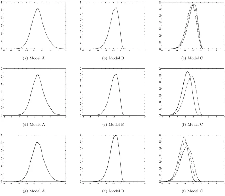
Figures 1 to 3 report asymptotic densities for CA, BLS and W E statistics under the breaks

scenarios described in Section 3.2. CA and BLS densities are plotted together because, as

expected by the theory, these test statistics show the same asymptotic distribution.

Many interesting features arise. First, all figures highlight the symmetry of distributions

around the median break (λ= 50%). This leads to distributions with fatter right tails for CA

and BLS test statistics when breaks (in level and trend) take place asymmetrically around the

middle-point of the sample. This feature is mainly displayed for Model A and C in Figure 1, while for Model B (multiple level breaks with trend) asymptotic densities appear mostly unaffected by the number and location of breaks in the sample. Second, looking at Figures 2

and 3, we do observe two key features of theW E test statistics. The first one, is the invariance

of their asymptotic distribution, independently on the number and location of level breaks (Model A and B). This is consistent with the theoretical results presented by WE. However, this condition does not hold for Model C. In fact, when the DGP presents both level and trend breaks, asymptotic densities differ across simulations by the number and location of breaks. In

addition, the symmetry of distributions around the median break arise again (as for theCS and

BLS cases), but with a shift in the positive direction of the distribution as far as the breaks

are distributed asymmetrically in the sample. This feature then leads to different asymptotic critical values for Model C, depending on the number and location of breaks.

(19)

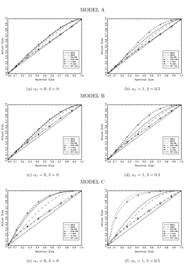
4.2 Empirical Size

We report in Tables 1 to 6 rejection frequencies at 5% nominal confidence level. The null

hypothesis is cointegration forCS and BLS tests and non-cointegration forW E tests. Results

are based on a single endogenous regressor xt (i.e., K = 1 and α1 = 1 in Equation (15)).

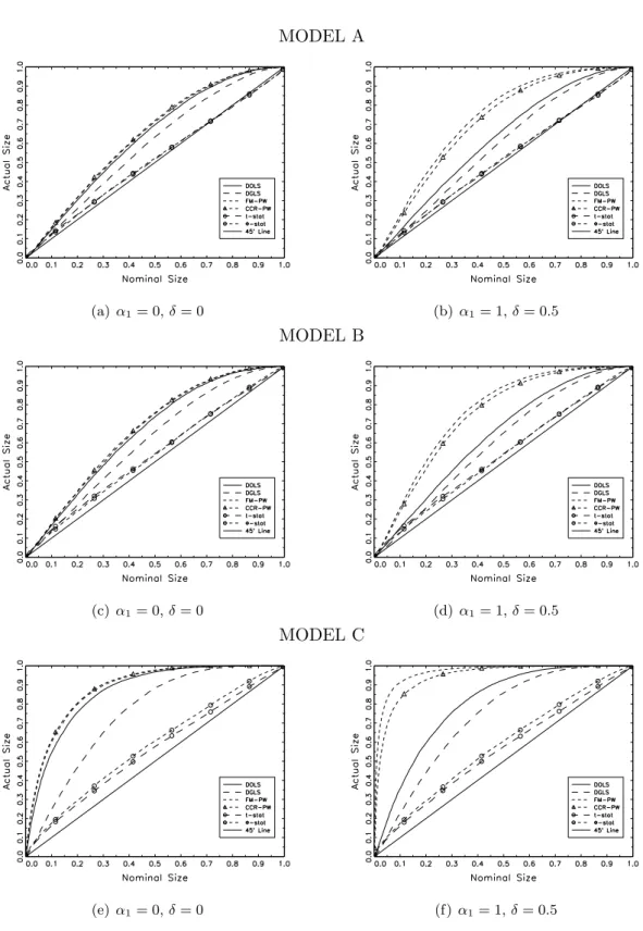
In Figures 4 to 6 we also report p-value plots of the empirical size of tests (Davidson and

MacKinnon, 1998) for the case that xt is endogenous (i.e., α1 = 1 and δ = 0.5) and strictly

exogenous (i.e., α1 = 0 andδ = 0). For reasons of space. we only report graphical results for

T = 100, φ=γ = 0 andσ2_µ= 2.

Asymptotic critical values are computed by simulating 40,000 series of dimension T∞ =

5,000 and picking up the 95th percentile of the asymptotic distribution for CS and BLS tests

and the 5th _{percentile for} _{W E} _tests.

4.2.1 One break (m= 1)

Results from the single break case are reported in Tables 1 (T = 100) and 2 (T = 200).

Forφ=γ = 0, we do not observe strong size distortions for all tests and Models, except for

some persistent under-rejection for the CSFM and BLSCCR tests when δ = 0.5. As expected,

tests display larger bias for lower signal-to-noise ratios. For largeσ_µ2,CSDOLSandCSDGLStests

show the strongest improvement in terms of rejection rates. When residuals are specified as an

AR(1) process (φ6= 0), CS andBLS tests show the highest rates of rejection in all models. In

particular, the CSDGLS test shows the strongest over-size (between 15% and 40%) in Model A

and C whenσ_µ2 is low. However, the displayed high rejection rate (or the discrepancy between

results for theCSDGLSand the other tests) is reduced in larger samples (Table 2). On the other

hand, theW EΦ test is affected by a persistent under-rejection bias, which seems to exacerbate

in larger samples. For the case of MA(1) residuals (γ 6= 0), actual size generally improves

with respect to the AR(1) specification. However, CSDOLS and CSDGLS tests are affected by

some under-rejection with large signal/noise ratios, while both W Et-stat and W EΦ tests tend

to over-reject instead.

P-value plots in Figure 4 show that actual rejection frequencies are very close to the

nom-inal size when the regressor is exogenous. In Model C, however, CS and BLS tests tend to

(20)

xt is endogenous can be found in Model C, where the over-rejection bias exacerbates forCSFM

and BLSCCR tests.

4.2.2 Three breaks (m= 3)

Results from the three breaks case are reported in Tables 3 (T = 100) and 4 (T = 200).

Simulations suggest that the inclusion of more breaks can significantly alter the size performance

of tests. In particular, tests based on non-parametric endogeneity-bias corrections (CSFM and

BLSCCR) display very large over-size when testing for cointegration in Model C.

As for the single break case, for φ = γ = 0 we do not observe strong size distortions for

all tests and Models. However, strong bias is displayed by CSDOLS, CSFM and BLSCCR tests

for Model C. In this case, the use of CSDGLS and W E tests is recommended. When residuals

are AR(1) (φ 6= 0), best results are obtained by CSFM and BLSCCR tests in Model A and

B, while the use of CSDOLS and CSDGLS tests is somewhat more recommended for Model C.

Nevertheless, results for larger samples (Table 4) display similar rejection rates across all CS

and BLS tests, in particular for higher signal-to-noise ratios. On the other hand, theW Et-stat

test is high performant across Models and specifications. When residuals are MA(1) (γ 6= 0),

CSDOLS andCSDGLS tests are generally well-sized in all Models, along with the W E tests.

P-value plots in Figure 5 highlight again the poor size performance of CSFM and BLSCCR

when the regressor is endogenous and the DGP presents a broken trend (Figure 4f). However,

a large oversize can be detected in Model C even when the regressor is exogenous (Figure 4e).

In this case,CSDOLS,CSFMandBLSCCRtests show the worst size distortion. When compared

to the endogenous case, we nevertheless observe an improvement in terms of p-values for the

CSDOLS test, while the performance ofCSFM and BLSCCR tests strongly deteriorates.

4.2.3 Five breaks (m= 5)

Results from the five breaks case are reported in Tables 5 (T = 100) and 6 (T = 200).

Sim-ulations remove any doubt about the evidence already reported above: the larger the number of breaks assumed in the DGP of the cointegrating process, the stronger the size bias affecting

the tests under analysis. An exception arise again for theW E tests, for which the inclusion of

(21)

the smallest over-rejection rates can be found for high signal-to-noise ratios in Model A and B.

This is not the case in Model C, where CS and BLS tests perform very badly, in particular

the CSFM and BLSCCR tests. However, strong size improvements can be obtained for larger

samples (see Table 6). In addition, it is worth noticing that the empirical size ofW Et-stat and

W EΦ lies between 5% and 10% in all Models. When residuals are AR(1) (φ6= 0), the smallest

size distortions are instead reported forCSDOLS,CSFMandBLSCCRstatistics in Model A and

B, mainly when δ >0. However, for small samples, these tests show very high over-rejection

rates, which are exacerbated in Model C. When residuals are MA(1) (γ 6= 0), the use ofCSDOLS

and CSDGLS, along with the W E tests, is strongly recommended in all Models whenT is low,

although the reported evidence of some under-rejection. However, as highlighted in Table 6,

CSFM and BLSCCR tests display strong size improvements in Model A and B when a larger

sample is considered, while they show huge over-rejection in Model C for all considered sample sizes.

The p-value analysis (Figure 6) confirms the results discussed above. It is interesting to

note that, as already observed in the 3 breaks case, the discrepancy arising from specifications involving either exogenous or endogenous regressors tends to widen with the number of breaks. However, over-rejection is high overall, whether the regressor is exogenous or not. In particular,

Model C shows the strongest bias in terms of p-value rejection probabilities. An interesting

feature is the diverging behaviour of CSDOLS, CSFM and BLSCCR tests observed in the

en-dogenous regressor specification: when compared to the case with exogenous regressors, for the first one the actual size improves, while for the last two tests it strongly deteriorates.

4.3 Empirical Power

We report in Tables 7 to 12 size-adjusted rejection frequencies at 5% actual confidence level.

The alternative hypothesis is non-cointegration for CS and BLS tests and cointegration for

W E tests. Critical values are computed by picking up the 95th percentile from the actual

distribution of CS and BLS tests and the 5th percentile from the actual distribution of W E

tests. For reasons of space, we only report power analysis for the case of correct specification of

residuals (γ =φ= 0). In Figures 7 to 9 we report power-size curves (Davidson and MacKinnon,

(22)

α1 = 0 and δ = 0).5 For this exercise, we use again the following parameter space: T = 100,

φ=γ= 0 and σ2_µ= 2.

4.3.1 One break (m= 1)

Results from the single break case are reported in Tables 7 (T = 100) and 8 (T = 200). Under

the alternative hypothesis, CS and BLS tests show a quite high power in Model A and C. In

particular, highest rejection rates are displayed by the CSDGLS test, lying between 40% and

65% and growing with higher signal-to-noise ratios. Largest rejection rates in Model B are

instead displayed by CSDOLS and CSFM tests. In addition, the former shows rejection rates

decreasing faster than in other tests when we move away from the alternative hypothesis of non-cointegration. For larger samples, all tests display similar rejection power, although the

CSDGLStest still shows a slight better performance in Model A and C. A very important result

is the serious low power across models and simulations for the W E tests. Rejection rates are

overall close to the nominal size (and even their empirical size), which makes these tests unable to reject the alternative hypothesis of cointegration. A larger sample size does not seem to improve these results.

Size-power curves in Figure 7 show that the latter result is mainly driven by the endogeneity

of regressors. When the regressor is strictly exogenous (Figure 7a, 7c and 7e), the W EΦ test

displays the highest power against the alternative hypothesis, while the W Et-stat is quite less

performant above the 10% nominal size. However, the endogeneity of regressors dramatically

alter their power (Figure 7b, 7dand 7f), whileCS andBLS tests appear mostly unaffected.

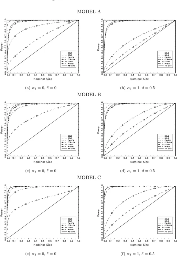
4.3.2 Three breaks (m= 3)

Results from the three breaks case are reported in Tables 9 (T = 100) and 10 (T = 200).

Results are somewhat different with respect to the single break case. The highest rejection

rates in Model A and B are displayed by the CSDGLS test, while in Model C the CSDOLS test

shows a slightly better power performance. However, rejection frequencies reported in Table

10 tend to be similar across tests and Models, except for the CSDOLS test in Model A and B.

Improved rejection power can be overall observed for higher signal-to-noise ratios and non-zero

5

It is worth noticing that results reported in Tables 7 to 12 are size-adjusted rejection frequencies, while

(23)

correlation between innovations (δ 6= 0). It is worth noticing that the more the number of breaks in the cointegrating model, the larger the size-adjusted power of tests. This is at odds with the evidence reported for the actual size of tests. However, this finding doesn’t hold for

W E tests, which still display rejection rates close to the nominal size.

Size-power curves in Figure 8 reveal that, with strictly exogenous regressors (Figure 8a, 8c

and 8e), theCSDGLStest displays the highest power against the alternative hypothesis in Model

A, while all tests show similar power in Model B and C, except for the W Et-stat test. When

the regressor is endogenous (Figure 8b, 8dand 8f),W E tests, however, lack power. Size-power

plots confirm results reported in Table 9, i.e., multiple breaks appear to improve the overall

power ofCS and BLS tests when compared to the single break case.

4.3.3 Five breaks (m= 5)

Finally, results from the five breaks case are reported in Tables 11 (T = 100) and 12 (T = 200).

As for the three breaks case, highest rejection rates in Model A and B are displayed by the

CSDGLStest, while in Model C theCSDOLSis somewhat more performant. It is worth noticing

that theCSFM displays very low rejection rates in Model C whenδ6= 0. However, as shown in

Table 12, this high power distortion is partially absorbed in larger samples. Finally, W E tests

show serious lack of power.

Size-power curves in Figure 9 reveal that, with strictly exogenous regressors (Figure 9a,

9c and 9e), all tests, except for the W Et-stat test, display high power against the alternative

hypothesis in Model A, B and C. However, when the regressor is endogenous (Figure 9b, 9d

and 9f), CS and BLS tests still display very high power, while W E tests show severe power

distortions.

5 Concluding Remarks

In this paper we compare the size-power performance of residual-based tests for cointegration with structural breaks. In particular, we focus on statistical tests recently proposed in the

litera-ture by Bartley, Lee, and Strazicich (2001), Carrion-i-Silvestre and Sans`o (2006) and Westerlund

and Edgerton (2007). Through an extensive Monte Carlo study, we evaluate their performance in small samples when up to five (exogenous) deterministic breaks are included in the

(24)

coin-tegrating equation. We consider several efficient estimators of single-equation coincoin-tegrating relationships (OLS, DOLS, DGLS, FM-OLS, CCR) and we design simulations to take into ac-count for three deterministic breaks scenarios (breaks in constant, with and without trend, and breaks in both constant and trend), endogenous regressors and residuals misspecifications.

Results on the empirical size reveal many interesting features. First, theW Et-stat andW EΦ

tests show quite low size distortions across Models and break scenarios. Findings reported in this study strongly recommend the use of these tests when estimates of cointegrating relationships

are conducted through the Engle-Granger OLS regression,i.e., when potential endogeneity bias

isex ante ruled out by the researcher. Second, multiple breaks tend to severely deteriorate the

size performance of the other tests under analysis. This finding appears even stronger in Model

C (level and trend breaks). Nevertheless, results for CS and BLS tests appear overall mixed

and can be briefly resumed in what follows.

For the single break case, when residuals are well-specified, CSDOLS and CSDGLS perform

best in all Models. However, theCSFM andBLSCCRtests show a slight lower size distortion in

Model C when residuals are misspecified. For the three breaks case, under white noise residuals,

we recommend the use of theCSDGLS test in Model C. When residuals are misspecified,CSFM

and BLSCCR tests perform best in Model A and B, while we recommend the use CSDOLS and

CSDGLS for Model C. For the five breaks case, we report large size distortions overall. Similar

performances are found out acrossCSDOLS,CSFM andBLSCCRtests in Model A and B, while

theCSDGLS test shows smaller (but still high) size distortions in Model C. With a sample size

of T = 100 used in simulations,CSFM and BLSCCR tests display impressive size distortions in

Model C. We then strongly advice against the use of these estimator/test pairs in a framework involving more then three level and trend breaks and less then 200 observations.

Despite the presence of strong size distortions, simulation results on the empirical

(size-adjusted) power reveal that (under white noise residuals) CS and BLS tests have quite high

power against the alternative hypothesis across all simulations and Models. In particular, the

CSDGLS displays overall best power performance in Model A and B, while the CSDOLS test

shows highest rejection rates in Model C. The severe lack of power ofW E tests when regressors

are endogenous (confirmed by size-power curves) should motivate their application for weak exogenous regression models only.

(25)

All in all, our results provide an important guideline for applied works involving cointe-grating models and multiple deterministic structural breaks. Unless the researcher deals with weakly exogenous regressors, in which case the SP-type LM tests proposed in Westerlund and Edgerton (2007) show impressive size and power performances, the KPSS-type LM tests

pro-posed by Carrion-i-Silvestre and Sans`o (2006) based on DGLS and DOLS estimators should be

used instead. This implies that the researcher should carefully select ex ante the estimator of

(26)

References

Ahn, S. K., 1993. Some tests for unit roots in autoregressive-integrated-moving average models with deterministic trends. Biometrika 80 (4), 855–868.

Andrews, D. W. K., 1991. Heteroskedasticity and autocorrelation consistent covariance matrix estimation. Econometrica 59 (3), 817–858.

Andrews, D. W. K., Monahan, J. C., 1992. An improved heteroskedasticity and autocorrelation consistent covariance matrix estimator. Econometrica 60 (4), 953–966.

Bai, J., Perron, P., 1998. Estimating and testing linear models with multiple structural changes. Econometrica 66 (1), 47–78.

Bai, J., Perron, P., 2003. Computation and analysis of multiple structural-change models. Jour-nal of Applied Econometrics 18 (1), 1–22.

Bartley, W. A., Lee, J., Strazicich, M. C., 2001. Testing the null of cointegration in the presence of a structural break. Economics Letters 73 (3), 315–323.

Campbell, J., Perron, P., 1991. Pitfalls and Opportunities: What Macroeconomists Should Know about Unit Roots. In: Blanchard, O. and Fisher, S. (eds.), NBER Macroeconomics Annual. MIT Press: Cambridge, MA (USA).

Carrion-i-Silvestre, J. L., Kim, D., Perron, P., 2009. GLS-based unit root tests with multiple structural breaks both under the null and the alternative hypothesis. Econometric Theory 25 (6), 1754–1792.

Carrion-i-Silvestre, J. L., Sans`o, A., 2006. Testing the null of cointegration with structural

breaks. Oxford Bulletin of Economics and Statistics 68 (5), 623–646.

Cheung, Y., Lai, K. S., 1993. Long-run purchasing power parity during the recent float. Journal of International Economics 34 (1-2), 181–192.

Choi, I., Ahn, B. C., 1995. Testing for cointegration in a system of equations. Econometric Theory 11 (5), 952–983.

Davidson, R., MacKinnon, J. G., 1998. Graphical methods for investigating the size and power of hypothesis tests. The Manchester School of Economic & Social Studies 66 (1), 1–26. De Peretti, C., Urga, G., 2004. Stopping tests in the sequential estimation of multiple structural

breaks. Econometric Society 2004 Latin American Meetings No. 320, Econometric Society. Engle, R. F., Granger, C. W. J., 1987. Cointegration and error correction: Representation,

estimation and testing. Econometrica 55 (2), 251–276.

Granger, C. W. J., Lee, T. H., 1990. Multicointegration. Advances in Econometrics 8, 71–84. Gregory, A. W., Hansen, B. E., 1996. Residual-based tests for cointegration in models with

regime shifts. Journal of Econometrics 70 (1), 99–126.

Hansen, B. E., 1992. Tests for parameter instability in regressions with I(1) processes. Journal of Business & Economic Statistics 10 (3), 321–335.

(27)

Hao, K., 1996. Testing for structural change in cointegrated regression models: Some compar-isons and generalizations. Econometric Reviews 15 (4), 401–429.

Harvey, D. I., Leybourne, S. J., Taylor, A. M. R., 2009a. Robust methods for detecting multi-ple level breaks in autocorrelated time series. Granger Centre Discussion Paper No. 09/01, University of Nottingham (UK).

Harvey, D. I., Leybourne, S. J., Taylor, A. M. R., 2009b. Simple, robust and powerful tests of the breaking trend hypothesis. Econometric Theory 25 (4), 995–1029.

Haug, A. A., 1996. Tests for cointegration: a Monte Carlo comparison. Journal of Econometrics 71 (1-2), 89–115.

Hendry, D. F., Ericsson, N. R., 1991. An econometric analysis of the UK money demand in “Monetary trends in the United States and the United Kingdom” by Milton Friedman and Anna J. Schwartz. American Economic Review 81 (1), 8–38.

Herrndorf, N., 1984. A functional central limit theorem for weakly dependent sequences of random variables. Annals of Probability 12 (1), 141–153.

Kejriwal, M., Lopez, C., 2010. Unit roots, level shifts and trend breaks in per capita output: A robust evaluation. Economics Working Papers No. 2010-02, University of Cincinnati (USA). Kejriwal, M., Perron, P., 2008. Data dependent rules for selection of the number of leads and

lags in the dynamic OLS cointegrating regression. Econometric Theory 24 (5), 1425–1441. Kejriwal, M., Perron, P., 2009a. A sequential procedure to determine the number of breaks

in trend with an integrated or stationary noise component. Economics Working Papers No. 1217, Purdue University (USA).

Kejriwal, M., Perron, P., 2009b. Testing for multiple structural changes in cointegrated regres-sion models. Journal of Business & Economic Statistics (forthcoming).

King, R. G., Plosser, C. I., Stock, J. H., Watson, M. W., 1991. Stochastic trends and economic fluctuations. American Economic Review 81 (4), 819–840.

Kurozumi, E., 2002. Testing for stationarity with a break. Journal of Econometrics 108 (1), 63–99.

Kwiatkowski, D., Phillips, P., Schmidt, P., Shin, Y., 1992. Testing the null hypothesis of sta-tionarity against the alternative of a unit root: How sure are we that economic time series have a unit root? Journal of Econometrics 54 (1-3), 159–178.

Lee, J., 1999. Stationarity Tests with Multiple Endogenized Breaks. In: Rothman, P. (ed.), Non-linear Time Series Analysis of Economic and Financial Data. Kluwer Academic Publishers. McCabe, B. P. M., Leybourne, S. J., Shin, Y., 1997. A parametric approach to testing the null

of cointegration. Journal of Time Series Analysis 18 (4), 395–413.

Mogliani, M., Urga, G., Winograd, C., 2009. Monetary disorder and financial regimes: the demand for money in Argentina, 1900-2006. PSE Working Papers No. 2009-55, Paris School of Economics (France).

Ng, S., Perron, P., 1995. Unit root tests in ARMA models with data-dependent methods for the selection of the truncation lag. Journal of the American Statistical Association 90, 269–281.

(28)

Park, J. Y., 1992. Canonical cointegrating regressions. Econometrica 60 (1), 119–143.

Perron, P., 1989. The great crash, the oil price shock and the unit root hypothesis. Econometrica 57 (6), 1361–1401.

Perron, P., 1990. Testing for a unit root in a time series with a changing mean. Journal of Business & Economic Statistics 8 (2), 153–162.

Perron, P., Yabu, T., 2009. Testing for shifts in trend with an integrated or stationary noise component. Journal of Business & Economic Statistics 27 (3), 369–396.

Perron, P., Zhu, X., 2005. Structural breaks with deterministic and stochastic trends. Journal of Econometrics 129 (1-2), 65–119.

Phillips, P. C. B., Durlauf, S. N., 1986. Multiple time series regression with integrated processes. Review of Economic Studies 53 (4), 473–495.

Phillips, P. C. B., Hansen, B. E., 1990. Statistical inference in instrumental variables regression with I(1) processes. Review of Economic Studies 57 (1), 99–125.

Phillips, P. C. B., Ouliaris, S., 1990. Asymptotic properties of residual based tests for cointe-gration. Econometrica 58 (1), 165–193.

Phillips, P. C. B., Sul, D., 2003. Dynamic panel estimation and homogeneity testing under cross section dependence. The Econometrics Journal 6 (1), 217–260.

Qu, Z., 2007. Searching for cointegration in a dynamic system. Econometrics Journal 10 (3), 580–604.

Saikkonen, P., 1991. Asymptotically efficient estimation of cointegration regressions. Economet-ric Theory 7 (1), 1–21.

Schmidt, P., Phillips, P. C. B., 1992. LM tests for a unit root in the presence of deterministic trends. Oxford Bulletin of Economics and Statistics 54 (3), 257–287.

Shin, Y., 1994. A residual-based test of the null of cointegration against the alternative of non-cointegration. Econometric Theory 10 (1), 91–115.

Stock, J. H., Watson, M. W., 1993. A simple estimator of cointegrating vectors in higher order integrated systems. Econometrica 61 (4), 783–820.

Sul, D., Phillips, P. C. B., Choi, C. Y., 2005. Prewhitening bias in HAC estimation. Oxford Bulletin of Economics and Statistics 67 (4), 517–546.

Taylor, M. P., McMahon, P. C., 1988. Long-run purchasing power parity in the 1920s. European Economic Review 32 (1), 179–197.

Westerlund, J., Edgerton, D. L., 2007. New improved tests for cointegration with structural breaks. Journal of Time Series Analysis 28 (2), 188–224.

(29)

Figure 1: Asymptotic Densities of CS and BLS Statistics.

(a) Model A (b) Model B (c) Model C

(d) Model A (e) Model B (f) Model C

(g) Model A (h) Model B (i) Model C

Notes: Kernel densities are obtained by simulating 40,000 series of dimensionT∞= 5,000

Panels (a), (b) and (c) are the 1 break model. Solid line: λ= 10%. Dashed line: λ= 20%. Short dashed line: λ= 40%. Dotted and dashed line: λ= 50%.

Panels (d), (e) and (f) are the 3 breaks model. Solid line: λ= {30%,50%,70%}. Dashed line: λ ={20%,50%,80%}. Short dashed line:λ={10%,20%,30%}. Dotted and dashed line: λ={70%,80%,90%}.

Panels (g), (h) and (i) are the 5 breaks model. Solid line: λ = {20%,30%,50%,70%,80%}. Dashed line: λ =

{30%,40%,50%,60%,70%}. Short dashed line: λ = {10%,20%,30%,40%,50%}. Dotted and dashed line: λ =

(30)

Figure 2: Asymptotic Densities ofW EΦ Statistic.

(31)

Figure 3: Asymptotic Densities of W Et-stat Statistic.

(32)

Figure 4: P-value Plots: 1 break MODEL A (a)α1= 0,δ= 0 (b) α1= 1,δ= 0.5 MODEL B (c) α1= 0,δ= 0 (d) α1= 1,δ= 0.5 MODEL C (e) α1 = 0,δ= 0 (f)α1= 1,δ= 0.5

Notes: Asymptotic distributions are obtained by simulating 20,000 series of dimension T∞ = 2,000.

Montecarlo simulations are obtained by simulating 20,000 series of dimension T = 100. λ = 50%,

(33)

Figure 5: P-value Plots: 3 breaks MODEL A (a)α1= 0,δ= 0 (b) α1= 1,δ= 0.5 MODEL B (c) α1= 0,δ= 0 (d) α1= 1,δ= 0.5 MODEL C (e) α1 = 0,δ= 0 (f)α1= 1,δ= 0.5

Montecarlo simulations are obtained by simulating 20,000 series of dimension T = 100. λ =

(34)

Figure 6: P-value Plots: 5 breaks MODEL A (a)α1= 0,δ= 0 (b) α1= 1,δ= 0.5 MODEL B (c) α1= 0,δ= 0 (d) α1= 1,δ= 0.5 MODEL C (e) α1 = 0,δ= 0 (f)α1= 1,δ= 0.5

(35)

Figure 7: Size-Power Curves: 1 break MODEL A (a)α1= 0,δ= 0 (b) α1= 1,δ= 0.5 MODEL B (c) α1= 0,δ= 0 (d) α1= 1,δ= 0.5 MODEL C (e) α1 = 0,δ= 0 (f)α1= 1,δ= 0.5

Montecarlo simulations are obtained by simulating 20,000 series of dimension T = 100. λ = 50%,

(36)

Figure 8: Size-Power Curves: 3 breaks MODEL A (a)α1= 0,δ= 0 (b) α1= 1,δ= 0.5 MODEL B (c) α1= 0,δ= 0 (d) α1= 1,δ= 0.5 MODEL C (e) α1 = 0,δ= 0 (f)α1= 1,δ= 0.5

(37)

Figure 9: Size-Power Curves: 5 breaks MODEL A (a)α1= 0,δ= 0 (b) α1= 1,δ= 0.5 MODEL B (c) α1= 0,δ= 0 (d) α1= 1,δ= 0.5 MODEL C (e) α1 = 0,δ= 0 (f)α1= 1,δ= 0.5

(38)

T able 1: Empirical Size (5% nominal size), 1 Break, λ = 50%, T = 100 MODEL A CS (2006) BLS (2001) WE (2007) C SDOLS C SDGLS C SFM B LS CCR W Et -stat W EΦ φ γ σ 2/δµ 0 0.5 0 0.5 0 0.5 0 0.5 0 0.5 0 0.5 0 0 0.5 0.0822 0.0682 0.1012 0 .0 620 0.0706 0.0219 0.0636 0.0207 0.0738 0.0735 0.0642 0.0663 1 0.0743 0.0649 0.0566 0 .0 462 0.0543 0.0221 0.0562 0.0252 0.0722 0.0718 0.0656 0.0659 2 0.0660 0.0505 0.0467 0 .0 383 0.0520 0.0257 0.0554 0.0277 0.0721 0.0714 0.0648 0.0627 0.4 0 0.5 0.1047 0.0756 0.4026 0 .1 798 0.1142 0.0335 0.1098 0.0411 0.0655 0.0681 0.0364 0.0481 1 0.0962 0.0756 0.2196 0 .0 817 0.0972 0.0434 0.0984 0.0516 0.0678 0.0668 0.0295 0.0307 2 0.0966 0.0734 0.1372 0 .0 583 0.0948 0.0600 0.0950 0.0648 0.0697 0.0697 0.0205 0.0164 0 0.4 0.5 0.0501 0.0431 0.0304 0 .0 286 0.0513 0.0261 0.0221 0.0145 0.0734 0.0746 0.0876 0.0767 1 0.0314 0.0262 0.0189 0 .0 207 0.0297 0.0184 0.0190 0.0155 0.0755 0.0773 0.1063 0.1063 2 0.0174 0.0158 0.0147 0 .0 151 0.0213 0.0154 0.0193 0.0150 0.0801 0.0866 0.1327 0.1648 MODEL B CS (2006) BLS (2001) WE (2007) C SDOLS C SDGLS C SFM B LS CCR W Et -stat W EΦ φ γ σ 2/δµ 0 0.5 0 0.5 0 0.5 0 0.5 0 0.5 0 0.5 0 0 0.5 0.1089 0.0894 0.1122 0 .0 734 0.1025 0.0397 0.0853 0.0331 0.0826 0.0812 0.0719 0.0710 1 0.0907 0.0761 0.0694 0 .0 541 0.0721 0.0329 0.0699 0.0350 0.0813 0.0816 0.0742 0.0737 2 0.0735 0.0517 0.0545 0 .0 412 0.0576 0.0325 0.0612 0.0350 0.0816 0.0807 0.0717 0.0702 0.4 0 0.5 0.1640 0.1141 0.2842 0 .1 572 0.1472 0.0527 0.1414 0.0606 0.0732 0.0756 0.0388 0.0509 1 0.1379 0.0976 0.2047 0 .0 912 0.1213 0.0540 0.1190 0.0621 0.0723 0.0703 0.0293 0.0304 2 0.1227 0.0821 0.1492 0 .0 657 0.1015 0.0639 0.1062 0.0680 0.0747 0.0721 0.0196 0.0160 0 0.4 0.5 0.0610 0.0557 0.0376 0 .0 386 0.1120 0.0639 0.0380 0.0217 0.0846 0.0815 0.1026 0.0866 1 0.0377 0.0319 0.0261 0 .0 273 0.0618 0.0363 0.0288 0.0228 0.0936 0.0920 0.1278 0.1254 2 0.0198 0.0187 0.0168 0 .0 174 0.0389 0.0255 0.0283 0.0234 0.1000 0.1130 0.1598 0.1977 MODEL C CS (2006) BLS (2001) WE (2007) C SDOLS C SDGLS C SFM B LS CCR W Et -stat W EΦ φ γ σ 2/δµ 0 0.5 0 0.5 0 0.5 0 0.5 0 0.5 0 0.5 0 0 0.5 0.1135 0.0873 0.1347 0 .0 827 0.1413 0.0560 0.1254 0.0506 0.0840 0.0818 0.0741 0.0746 1 0.0952 0.0811 0.0750 0 .0 557 0.0900 0.0418 0.0921 0.0430 0.0833 0.0816 0.0767 0.0757 2 0.0818 0.0546 0.0571 0 .0 389 0.0664 0.0347 0.0730 0.0383 0.0891 0.0858 0.0789 0.0757 0.4 0 0.5 0.1905 0.1171 0.4069 0 .2 254 0.2204 0.0719 0.2219 0.0990 0.0724 0.0750 0.0358 0.0524 1 0.1605 0.1023 0.2647 0 .1 084 0.1696 0.0735 0.1733 0.0896 0.0759 0.0736 0.0282 0.0295 2 0.1504 0.0972 0.1777 0 .0 794 0.1482 0.0846 0.1534 0.0945 0.0783 0.0784 0.0209 0.0159 0 0.4 0.5 0.0552 0.0502 0.0313 0 .0 318 0.2059 0.1731 0.0637 0.0703 0.0864 0.0839 0.1093 0.0911 1 0.0311 0.0257 0.0186 0 .0 196 0.1130 0.1105 0.0430 0.0601 0.0944 0.0910 0.1378 0.1322 2 0.0151 0.0137 0.0134 0 .0 118 0.0635 0.0658 0.0357 0.0517 0.1031 0.1180 0.1761 0.2169 Notes: The DGP is giv en in equations (12)-(16). xt is endogenous ( α1 = 1), α2 = − 1, ρ = 0 under H 0 for the C S and B LS tests, w h ile ρ = 1 under H 0 for the W E tests. The LR V is computed as in Kurozumi (2002). Asymptot ic critical v al ues are obtained b y sim ulating 40 , 000 series of dimension T∞ = 5 , 000. Estimated critical v alues for Mo del A are: 95% cv C S = B LS = 0.1552; 5% cv t -stat = -2.871, 5% cv Φ = -14.206. Estimated critical v alues for Mo del B are: 95% cv C S = B LS = 0.1057; 5% cv t -stat = -3.019, 5% cv Φ = -18. 150. Estimated critical v alues for Mo del C are: 95% cv C S = B LS = 0.0557; 5% cv t -stat = -3.333, 5% c v Φ = -22.084.

(39)

T able 2: Empirical Size (5% nominal size), 1 Break, λ = 50%, T = 200 MODEL A CS (2006) BLS (2001) WE (2007) C SDOLS C SDGLS C SFM B LS CCR W Et -stat W EΦ φ γ σ 2/δµ 0 0.5 0 0.5 0 0.5 0 0.5 0 0.5 0 0.5 0 0 0.5 0.0772 0.0732 0.0684 0 .0 549 0.0530 0.0180 0.0514 0.0184 0.0563 0.0565 0.0520 0.0534 1 0.0753 0.0671 0.0553 0 .0 504 0.0503 0.0244 0.0514 0.0249 0.0588 0.0568 0.0571 0.0536 2 0.0671 0.0566 0.0468 0 .0 435 0.0461 0.0256 0.0493 0.0259 0.0550 0.0599 0.0525 0.0558 0.4 0 0.5 0.0920 0.0794 0.2415 0 .0 946 0.0877 0.0248 0.0841 0.0276 0.0532 0.0540 0.0270 0.0374 1 0.0872 0.0746 0.1107 0 .0 641 0.0846 0.0417 0.0822 0.0442 0.0532 0.0513 0.0199 0.0214 2 0.0804 0.0733 0.0712 0 .0 532 0.0823 0.0600 0.0812 0.0610 0.0541 0.0568 0.0132 0.0133 0 0.4 0.5 0.0489 0.0490 0.0264 0 .0 305 0.0274 0.0107 0.0177 0.0087 0.0599 0.0558 0.0768 0.0649 1 0.0365 0.0312 0.0220 0 .0 246 0.0214 0.0137 0.0185 0.0113 0.0644 0.0638 0.0999 0.0969 2 0.0179 0.0168 0.0150 0 .0 156 0.0169 0.0115 0.0170 0.0111 0.0670 0.0752 0.1226 0.1506 MODEL B CS (2006) BLS (2001) WE (2007) C SDOLS C SDGLS C SFM B LS CCR W Et -stat W EΦ φ γ σ 2/δµ 0 0.5 0 0.5 0 0.5 0 0.5 0 0.5 0 0.5 0 0 0.5 0.0898 0.0762 0.0825 0 .0 578 0.0618 0.0255 0.0591 0.0238 0.0632 0.0600 0.0582 0.0563 1 0.0816 0.0723 0.0635 0 .0 549 0.0534 0.0303 0.0565 0.0294 0.0650 0.0643 0.0607 0.0604 2 0.0697 0.0579 0.0489 0 .0 466 0.0491 0.0309 0.0534 0.0317 0.0678 0.0661 0.0632 0.0612 0.4 0 0.5 0.1170 0.0938 0.2400 0 .1 029 0.1014 0.0321 0.0988 0.0331 0.0527 0.0551 0.0268 0.0384 1 0.1064 0.0857 0.1304 0 .0 711 0.0934 0.0477 0.0920 0.0496 0.0517 0.0545 0.0196 0.0218 2 0.0943 0.0776 0.0881 0 .0 566 0.0868 0.0628 0.0866 0.0643 0.0581 0.0600 0.0126 0.0098 0 0.4 0.5 0.0538 0.0509 0.0301 0 .0 319 0.0512 0.0239 0.0238 0.0124 0.0683 0.0635 0.0882 0.0714 1 0.0389 0.0334 0.0265 0 .0 281 0.0329 0.0215 0.0237 0.0165 0.0760 0.0742 0.1161 0.1144 2 0.0198 0.0202 0.0169 0 .0 189 0.0250 0.0170 0.0220 0.0161 0.0872 0.0970 0.1547 0.1928 MODEL C CS (2006) BLS (2001) WE (2007) C SDOLS C SDGLS C SFM B LS CCR W Et -stat W EΦ φ γ σ 2/δµ 0 0.5 0 0.5 0 0.5 0 0.5 0 0.5 0 0.5 0 0 0.5 0.0992 0.0843 0.0911 0 .0 664 0.0669 0.0221 0.0678 0.0215 0.0671 0.0662 0.0622 0.0625 1 0.0914 0.0769 0.0638 0 .0 529 0.0559 0.0246 0.0632 0.0261 0.0659 0.0641 0.0623 0.0605 2 0.0816 0.0664 0.0530 0 .0 491 0.0525 0.0269 0.0597 0.0297 0.0675 0.0682 0.0632 0.0627 0.4 0 0.5 0.1341 0.1023 0.3209 0 .1 374 0.1407 0.0369 0.1348 0.0402 0.0558 0.0585 0.0281 0.0403 1 0.1178 0.0945 0.1619 0 .0 790 0.1211 0.0550 0.1170 0.0582 0.0557 0.0554 0.0187 0.0197 2 0.1105 0.0923 0.1059 0 .0 649 0.1132 0.0794 0.1116 0.0807 0.0584 0.0588 0.0121 0.0089 0 0.4 0.5 0.0510 0.0497 0.0237 0 .0 275 0.0648 0.0344 0.0198 0.0134 0.0708 0.0672 0.0929 0.0770 1 0.0325 0.0255 0.0166 0 .0 188 0.0357 0.0211 0.0179 0.0150 0.0757 0.0736 0.1237 0.1191 2 0.0137 0.0133 0.0129 0 .0 124 0.0233 0.0154 0.0197 0.0150 0.0889 0.1024 0.1678 0.2139 Notes: See T able 1.