IMPROVED ESTIMATION OF FLEXIBLE LOGIT
MODELS AND AN EXTENSION TO A MODEL
WITH A T-DISTRIBUTED ERROR KERNEL
A Dissertation
Presented to the Faculty of the Graduate School of Cornell University
in Partial Fulfillment of the Requirements for the Degree of Doctor of Philosophy
by Prateek Bansal
c
2019 Prateek Bansal ALL RIGHTS RESERVED
IMPROVED ESTIMATION OF FLEXIBLE LOGIT MODELS AND AN EXTENSION TO A MODEL WITH A T-DISTRIBUTED ERROR KERNEL
Prateek Bansal, Ph.D. Cornell University 2019
Understanding various micro-decisions of travelers (e.g., choice of vehicles, travel modes, or destinations) is of utmost importance in travel demand modeling. Af-ter the first application of the multinomial logit model in the early 1970s, micro-econometric models to elicit these type of choices have evolved in mainly two ways: a) computationally efficient estimation (e.g., fast integral approximations); and b) behaviorally defensible models (e.g., modeling preference heterogeneity).
This dissertation contributes to both lines of behavior modeling research — whereas chapters one to three analyze and improve the computational efficiency of flexible logit models and the required approximation of high-dimensional integrals, chapter four derives the first multinomial response model with a t-distributed error kernel that accounts fordecision uncertaintybehavior of travelers. A summary of each chapter is provided below.
InChapter 1, we extend the logit-mixed logit (LML) model, an advanced semi-parametric specification of preference heterogeneity, to a combination of fixed and random parameters. We show that the likelihood of the LML specification loses its special properties due to the inclusion of fixed parameters, leading to a much higher estimation time. In an empirical application about preferences for alterna-tive fuel vehicles in China, estimation time increased by a factor of 20-40 when
introducing fixed parameters. Despite losses in computation efficiency, we show that the flexible LML could retrieve multimodal mixing distributions.
InChapter 2, we derive, implement, and test minorization-maximization (MM) algorithms to estimate the semiparametric LML and mixture-of-normals multino-mial logit (MON-MNL) models. In a Monte Carlo study and empirical application to estimate consumer’s willingness to adopt electric motorcycles in Indonesia, we compare the maximum simulated likelihood estimator (MSLE) with the derived MM algorithms. Whereas in LML estimation MM is computationally noncom-petitive with MSLE, it is a comnoncom-petitive replacement to MSLE for MON-MNL that obviates computation of complex analytical gradients.
InChapter 3, we propose the application of a moment-based designed quadra-ture (DQ) method to approximate multi-dimensional integrals in MSLE of discrete choice models. The results of simulation study indicate that DQ is a potentially attractive alternative to quasi-Monte Carlo (QMC) because it requires fewer eval-uations of the conditional likelihood (i.e., lower computation time) as compared to QMC methods, is as easy to implement, ensures positivity of weights, and can be created on any general polynomial spaces. Finally, we validate the performance of DQ on a case study to understand preferences for mobility-on-demand services in New York City.
InChapter 4, we demonstrate that using a t-distributed error kernel in multino-mial choice models helps in better predicting the preferences in class-imbalance datasets. This specification also implicitly accounts for the consumers’decision un-certaintybehavior. Because of these statistical and behavioral advantages, we
de-rive the first multinomial response model with a t-distributed error kernel and ex-tend this to a generalized continuous-multinomial (GCM) model. In the empirical study related to the adoption of electric vehicles (EVs), we observe that accounting fordecision uncertaintybehavior in the GCM model with t-distributed error kernel results into a higher willingness to pay for improving the EV attributes than those of a GCM model with a normally-distributed error kernel. These differences are relevant in making policies to expedite the market penetration of EVs.
BIOGRAPHICAL SKETCH
Having grown up in densely populated cities across India, Prateek have experi-enced the challenges that delays and overcrowding in rails pose on the day-to-day lives of people. This, in turn, motivated him to pursue research in Transportation Economics and Engineering.
Before joining Cornell, Prateek received his M.S. from The University of Texas at Austin in Transportation Engineering and B.Tech. from Indian Institute of Tech-nology (IIT) Delhi in Civil Engineering. Over the years he has also collaborated with researchers across different settings (e.g., Canada, Chile, South Africa, Swe-den, Taiwan, and the United States) on diverse transportation-related projects.
His pre-doctoral research experiences made him realize that system-level de-cisions can be better informed by eliciting and aggregating individual’s travel preferences. This helped him in focusing his doctoral research on advancing the micro-econometric models of consumer choice.
His current research interests are inter-disciplinary and broadly revolve around: i) bridging machine learning and econometrics, i.e. deriving computationally-efficient estimators of econometric models using approximate Bayesian inference; ii) addressing commonly ignored endogeneity concerns in multinomial choice models using partial identification; iii) understanding the im-pact of discrete choice experiment designs on the modeling results.
ACKNOWLEDGEMENTS
I take this opportunity to thank my mentors, collaborators, funding agencies, friends, and family, whose guidance and/or unconditional support have helped me sail through my doctoral journey.
My PhD committee has been very supportive throughout these years. I can-not thank Dr Ricardo Daziano (committee chair) enough for believing in my ideas and providing optimal freedom and time to pursue them. I would cherish his prompt feedback on research papers and our discussions during lunch meetings. He ensured that I acquire all the required skills and experiences to become a well-rounded academic researcher – suggested right course sequences, supported col-laborations through conference visits and university exchanges, and provided op-portunities to teach graduate classes and to write grant proposals. In addition, advanced econometrics courses taught by Drs Shanjun Li and Thomas DiCiccio have played a crucial role in setting the required foundation to start my research early. I am particularly thankful to them for providing statistical insights to han-dle various research problems that I encountered during my PhD.
Among other mentors, I am obliged to Prof. Kenneth Train for constantly ac-knowledging, reviewing, and encouraging my ideas, to Prof. Michel Bierlaire and Drs Ricardo Hurtubia, Taha Rashidi, Samitha Samaranayake, Erick Guerra, and Martin Achtnicht for providing survey data and/or detailed assessment of my work, to Prof. Kara Kockelman and Dr Stephen Boyles for teaching me funda-mentals of research and making me realize my abilities as a researcher, and to Profs. Geetam Tiwari, Mu Chen Chen and Robert Chapleau for providing me
with a platform to pursue my passion for transportation science during my un-dergraduate research. Additionally, semester exchange experiences at the Univer-sity of California, Berkeley and the UniverUniver-sity of Santiago, Chile have offered me unique exposure to multicultural research environments. I am grateful to Prof. Joan Walker, Dr Angelo Guevara, and Dr Alejandro Tirachini for hosting me and providing with such opportunities. I have been privileged to collaborate with multiple researchers during my PhD. Working with Yang, Rico, Rubal, Naveen, Tomas, and Subodh on multi-disciplinary problems have helped me learning var-ious dimensions of research such as remote collaborations and patiently progress-ing multiple projects simultaneously. Such collaborations also resulted in prolific research output, thanks to my efficient collaborators.
I also acknowledge financial support for my graduate research, conference travel, and semester exchanges from the National Science Foundation, the Cornell Graduate School, the International Institute of Forecasters, and the King Abdullah Petroleum Studies and Research Center. However, any errors that remain are my sole responsibility.
I am blessed to have a close-knit circle of friends who enabled me to sustain moving-forward attitude during these years. Naveen has always been available to discuss any kind of professional and personal challenges. His invaluable guid-ance has shaped various aspects of my personality. Without his support, I could not have achieved even three-fourths of what I did in PhD. Yogesh has always been a great source of inspiration and kept alive my belief in hard work. Being seniors in the same discipline, Tarun, Prasad, and Rahul specifically helped in
making various academic decisions. I am also thankful to other friends at Cor-nell – Abhi, Seema, Udit, Prankur, Gargi, Jessica, Vidya, Payal, Rohil, Mathew, Anaka, Karen, Nima, Raashid, Faisal, Will, and Sophia – who ensured a vibrant life besides work by organizing house parties, potlucks, and much more. Aditya, Praveen, Saqib, Surabhi, Oscar, Mengqiao, and Mostafa made Berkeley feel like home during my exchange. Esteban, Felipe, Kim, Diego, Javiera, Jacqueline, Is-abelle, Nico, Raul, Alisson, and Hans put a collective effort to make my visit to Chile memorable by providing authentic Latino experiences – from teaching me Spanish to hosting at family house parties. I am grateful to have friends like Averi, Kratika, Nikit, Rajat, Sunay, Dheeraj, Rishabh, Prateek Raj, Kartik, TKS, and Rohit Prakash, who latently provided me mental strength during tough times. Above all, I am fortunate to have parents and sister who absorbed financial adversities, trusted my decisions, and gave me the freedom to carve out my own path. This dissertation is dedicated to their sacrifices and unconditional love.
TABLE OF CONTENTS
Biographical Sketch . . . iii
Dedication . . . iv
Acknowledgements . . . v
Table of Contents . . . viii
List of Tables . . . xi
List of Figures . . . xiii
1 Extending the Logit-Mixed Logit Model for a Combination of Random and Fixed Parameters 1 1.1 Introduction: flexible mixing distributions . . . 1
1.2 Incorporating a subset of fixed parameters in logit-mixed logit models 5 1.2.1 Model Specification . . . 5
1.2.2 Maximum Likelihood Estimator . . . 7
1.2.3 Computational Efficiency of LML with all random and some fixed parameters . . . 8
1.3 Empirical Application . . . 9
1.3.1 Data Description . . . 10
1.3.2 Estimates . . . 12
1.4 Conclusions . . . 20
2 Minorization-Maximization (MM) Algorithms for Semiparametric Logit Models: Bottlenecks, Extensions, and Comparisons 22 2.1 Introduction . . . 22
2.1.1 Background . . . 22
2.1.2 Research Gap and Contribution . . . 26
2.2 Iterative Optimization Methods to Estimate the Logit Mixed Logit (LML) Model . . . 30
2.2.1 Logit-Mixed Logit (LML) . . . 30
2.2.2 LML Estimation using the EM Algorithm . . . 32
2.2.3 LML Estimation using the MM Algorithm . . . 34
2.2.4 LML Estimation using the Faster-MM Algorithm . . . 37
2.3 Iterative Optimization Methods to Estimate MON-MNL . . . 42
2.3.1 Mixture-of-normals logit (MON-MNL) . . . 42
2.3.2 MON-MNL Estimation using the EM Algorithm . . . 43
2.3.3 MON-MNL Estimation using the MM Algorithm . . . 44
2.3.4 MON-MNL Estimation using the faster-MM Algorithm. . . 45
2.4 Discussion: advantages and disadvantages of MM over EM and
MSLE . . . 49
2.5 Monte Carlo Study . . . 51
2.5.1 LML Monte Carlo Study . . . 53
2.5.2 MON-MNL Monte Carlo Study. . . 59
2.6 Empirical Study: Adoption of Electric Motorcycles . . . 67
2.7 Conclusions . . . 77
3 Designed Quadrature to Approximate Integrals in Maximum Simulated Likelihood Estimation 81 3.1 Introduction . . . 81
3.1.1 Quadrature Methods and Research Gap . . . 83
3.1.2 Moment-base Quadrature and Contributions . . . 85
3.2 Mixed Multinomial Logit Model . . . 87
3.3 Quadrature Methods . . . 89 3.3.1 Notation . . . 89 3.3.2 Univariate Quadrature . . . 91 3.3.3 Multivariate Quadrature . . . 92 3.3.4 Designed Quadrature (DQ) . . . 94 3.3.5 Discussion . . . 95
3.4 Monte Carlo Study . . . 97
3.4.1 Simulation Design . . . 97
3.4.2 Results and Discussion . . . 99
3.5 Empirical Study . . . 105
3.5.1 Experiment Design . . . 105
3.5.2 Estimation and Results . . . 107
3.6 Conclusions . . . 109
4 A Continuous-Multinomial Response Model with a t-distributed Error Kernel 111 4.1 Introduction . . . 111
4.2 Literature Review . . . 115
4.3 Methodology . . . 118
4.3.1 Continuous variable model . . . 118
4.3.2 Choice model . . . 119
4.3.3 Joint Model Specification . . . 120
4.3.4 Joint Model Estimation . . . 121
4.4.1 Class imbalance . . . 130
4.4.2 Behavioral implications . . . 131
4.5 Monte Carlo study and results . . . 135
4.5.1 Statistical properties of GCM-t estimator . . . 138
4.5.2 Effect of modeling fat-tailed data with normal distribution . 141 4.6 Empirical study . . . 143
4.6.1 Data description . . . 143
4.6.2 Results and discussion . . . 145
4.7 Conclusions and future work . . . 156
A Appendix of Chapter 1 170 A.1 Model Specification: Willingness to Pay Space . . . 170
A.2 Maximum Likelihood Estimator . . . 172
B Appendix of Chapter 2 173 C Appendix of Chapter 4 177 C.1 Matrix transformations . . . 177
C.1.1 Transformation matrix(D)to computeΛfromΛ . . . 177
C.1.2 Modified transformation matrix(Dm)to computeΣfromΣ . 180 C.1.3 Utility difference generator(M)to computeeΣfromΣ . . . . 181
C.1.4 Reparametrization of the Cholesky decomposition ofΣ . . . 182
LIST OF TABLES
1.1 Attributes and Levels for the Discrete Choice Experiment . . . 11 1.2 Estimation Results - All Random Parameters . . . 14 1.3 Estimation Results - Inclusion of ASCs and Fixed Parameters . . . 15 1.4 Estimation Results - Final Specification . . . 16 1.5 Comparing Computation Time of LML and LML-FR . . . 20 2.1 Preliminary Monte Carlo Simulation Results (LML Model) . . . 55 2.2 Monte Carlo Simulation Results (LML Model, N=500, Polynomial
Order=2) . . . 57 2.3 Monte Carlo Simulation Results (LML Model, N=500, Polynomial
Order=4) . . . 58 2.4 Monte Carlo Simulation Results (LML Model, N=2000, Polynomial
Order=2) . . . 58 2.5 Preliminary Monte Carlo Simulation Results (MMNL Model) . . . 61 2.6 Preliminary Monte Carlo Simulation Results (MON-MNL Model) 62 2.7 Monte Carlo Simulation Results (MON-MNL Model, N=2000, J=4) 64 2.8 Monte Carlo Simulation Results (MON-MNL Model, N=2000, J=50) 64 2.9 Monte Carlo Simulation Results (MON-MNL Model, N=500, J=50) 65 2.10 Monte Carlo Simulation Results (MON-MNL Model, N=500, J=100) 65 2.11 Standard Errors Comparison . . . 66 2.12 Summary of choice sets and attribute values . . . 68 2.13 Descriptive sample statistics (N=1208). . . 69 2.14 Adoption of Electric Motrocycles in Indonesia (MMNL Model
Re-sults) . . . 72 2.15 Adoption of Electric Motrocycles in Indonesia (LML Model Results) 73 2.16 Adoption of Electric Motrocycles in Indonesia (MON-MNL Model
Results) . . . 74 2.17 Computational Efficiency Ranking . . . 74 3.1 Comparison of DQ and MLHS (Monte Carlo, Random Parameters=3)101 3.2 Comparison of DQ and MLHS (Monte Carlo, Random Parameters=5)102 3.3 Comparison of DQ and MLHS (Monte Carlo, Random
Parame-ters=10) . . . 103 3.4 Experiment Design for Mode Choice Study . . . 106 3.5 Comparison of -Loglikelihood Values in the Case Study . . . 107 3.6 Comparison of Estimates and Standard Errors in the Case Study . 108
4.1 Class-imbalance example under Probit and t-distributed error kernel134 4.2 Simulation Results of GCM-t Model for DOF-I scenario (DOF=1) . 160 4.3 Simulation Results of GCM-t Model for DOF-II scenario (DOF=12) 161 4.4 Effect of ignoring non-normality (DOF=2) . . . 162 4.5 Effect of ignoring non-normality (DOF=12) . . . 163 4.6 Sample of a choice situation in the discrete choice experiment . . . 164 4.7 Descriptive statistics of the sample . . . 165 4.8 Comparison of GCM-t and GCM-N in empirical study (Part 1,
t-value in parenthesis) . . . 166 4.9 Comparison of GCM-t and GCM-N in empirical study (Part 2,
t-value in parenthesis) . . . 167 4.10 Degree-of-freedom specification results in GCM-t model (t-value
in parenthesis) . . . 168 4.11 Change in choice probability due to 1% reduction in parking-cost
of electric vehicle . . . 168 4.12 Change in choice probability due to 25% reduction in parking-cost
of electric vehicle . . . 169 4.13 Ratio of GCM-t and GCM-N probabilities for chosen alternative
for different DOF . . . 169 4.14 Covariance matrix (t-value in parenthesis) . . . 169 B.1 Lower Bound Approximation of Hessian: Simulation Results . . . 176
LIST OF FIGURES
1.1 Histogram of Marginal Utility of Purchase Price . . . 18
1.2 Histogram of Marginal Utility of Fuel Cost . . . 18
1.3 Histogram of Marginal Utility of Fuel Availability . . . 19
2.1 Histogram of Willingness to Pay (Rp. thousands) . . . 76
4.1 Cumulative density function of t- and normally-distributed ran-dom variables. . . 133
4.2 Willingness to pay to increase the driving range of an electric vehi-cle by a mile . . . 150
4.3 Probability of choosing electric vehicle due to change in utility of electric vehicle. . . 153
4.4 Probability of choosing gasoline vehicle due to change in utility of electric vehicle. . . 154
CHAPTER 1
EXTENDING THE LOGIT-MIXED LOGIT MODEL FOR A COMBINATION OF RANDOM AND FIXED PARAMETERS
1.1
Introduction: flexible mixing distributions
Analysts who model decision-making processes using random utility maximiza-tion theory cannot possibly include all relevant factors that affect choices. In fact, the decision-making process is generally heterogeneous. Heterogeneity may oc-cur due to taste variations in how decision makers weigh different attributes. Taste variations can be decomposed into observed and unobserved preference het-erogeneity. Whereas the standard conditional or multinomial logit (MNL) model (McFadden, 1973) can model observed preference heteorgeneity typically by in-teracting attributes with characteristics of the individual, unobserved preference heterogeneity requires further assumptions and a different model. To take into account unobserved preference heterogeneity, Boyd and Mellman (1980) intro-duced the mixed multinomial logit (MMNL) model by adding to MNL random parameters that follow a prespecified parametric, continuous mixing distribution. MMNL rapidly became standard practice in choice modeling research after the seminal paper byMcFadden and Train(2000), where the authors showed that any random utility maximization model can be approximated by MMNL, if mixing distributions of the random parameters are specified correctly.
In the MMNL literature, most studies have used normal or lognormal hetero-geneity distributions and a few have used gamma or triangular mixing. However, Louviere and Eagle (2006), Fosgerau and Hess (2007), and Louviere and Meyer (2008) have argued that the normal (and other parametric) mixing distributions may introduce problems of misspecification if the assumed distribution is not ap-propriate for the data; for example, researchers may obtain a negative marginal utility of income if a normal distribution is assumed (or any parametric distribu-tion with a possibly negative support). Bajari et al.(2007),Fosgerau and Bierlaire (2007),Train(2008),Bastin et al.(2010), Fox et al.(2011), andFosgerau and Mabit (2013) have specified non-parametric mixing distributions that are flexible and yet results into computationally less expensive estimation breaking down the tradi-tional flexibility versus ease of estimation tradeoff.
MMNL estimation is a nonlinear optimization problem, butBajari et al.(2007) proposed a method that is fast and easy to code that takes advantage of a linear-regression-type specification. The authors assume that the population can be sorted into finite classes or clusters (i.e. the number of preference parameters is discrete, c.f. the latent class logit specification: Kamakura and Russell, 1989; DeSarbo et al., 1995;Bhat, 1997) and assert that their estimator is non-parametric because any mixing distribution can be approximated by making the number of classes large enough. However, this linear regression method may violate some necessary constraints on the model parameters. To handle this issue, Fox et al. (2011) raparameterized MMNL and derived a specification very similar to that of Bajari et al.(2007), but used inequality constrained linear least squares.
Fos-gerau and Bierlaire(2007) further proposed a method to approximate any contin-uous distribution using Legendre polynomials. The use of polynomials is a very flexible simply because different distributions can be recovered by adding more terms to the series expansion. In addition,Train(2008) used computation-efficient expectation-maximization (EM) algorithms for non-parametric estimation of ran-dom parameter logit-type models (cf.Bhat,1997).
Train (2016) has very recently proposed the logit-mixed logit (LML) model, which is a generalized specification for all above four methods to generate mix-ing distributions.1 The logarithm of the mixing distribution can be easily spec-ified in LML, using splines, polynomials, step functions, and many other func-tional forms. Addifunc-tionally, a computafunc-tionally-convenient likelihood equation – that does not require computation of conditional choice probabilities in iterative optimization – significantly reduces estimation time of LML (see Section1.2.3for details). However, in its original formulation, LML assumes all utility parame-ters to be random. Note, however, that fixed parameparame-ters are usually needed in practice: a few of such instances are discussed below and illustrated in the em-pirical study. First, fixed alternative-specific constants (ASCs) should be included in the utility to account for alternative-specific fixed effects. Second, preferences 1However, note that Train (2016) does not generalize Bastin et al. (2010) andFosgerau and
Mabit(2013). Fosgerau and Mabit(2013) suggests to draw random numbers from some initial distribution(e.g., uniform) and transform these draws using a polynomial or other function to recover the mixing distribution. Similarly,Bastin et al.(2010) proposed a non-parametric method to approximate the inverse cumulative distribution function of the mixing distribution. They use a polynomial approximation (B-spline parameterization) of an initially chosen uniform distribution. A major limitation of these procedures is understanding the relationship between the shape of the mixing distribution and that of theinitial distributions.
for a specific covariate may not vary across individuals and thus the estimated parameter may be just non-random. Third, a parsimonious specification of het-erogeneity combines different means (deterministic taste variation) with the same variance of the unobserved part, by allowing the mean of a random parameter (e.g., marginal utility of price) to differ by socio-demographics (e.g., gender). This taste variation specification requires the inclusion of a fixed parameter on the in-teraction of the covariate with the demographic dummy (e.g., price × gender).
This chapter asserts that under a more general utility specification, i.e. utility with a combination of random and fixed parameters, the likelihood equation loses its computationally-convenient form, and thus LML exhibits major losses in compu-tational efficiency. In fact, the computation time of a model with a fixed parameter may be even 40 times higher than that of the case where all parameters are ran-dom (see Section 1.3.2for an example of this situation). This result is somewhat counter-intuitive because in parametric MMNL models assuming fixed parame-ters actually reduces computation time.
In sum, this chapter aims at: 1. Extending the LML model for a combination of random and fixed parameters (Section1.2); and 2. Providing an empirical applica-tion of our LML extension (Secapplica-tion1.3) – as case study we use stated preferences for alternative fuel vehicles in China. The original LML and our LML extension are used to fit models, and we compare the results with MNL and MMNL with normal heterogeneity (MMNL-N) models.
1.2
Incorporating a subset of fixed parameters in logit-mixed
logit models
1.2.1
Model Specification
Consider a standard discrete choice setting where individualn∈ {1, . . . ,N}chooses
one alternative from the mutually exclusive choice set {1, . . . ,J} (indexed by j) over the set of discrete time periods{1, . . . ,T}or choice situations (indexed byt). The random utility maximization model is specified as
Un jt =xn jt0βn+εn jt = h xFn jt0xRn jt0i βF βR n +εn jt (1.1)
where Un jt is the random indirect utility associated with individual n choosing alternative jduring choice situationt, andεn jt is an iid extreme value type I
pref-erence shock. Moreover, both the alternative attributes and prefpref-erence parame-ters are sorted in two groups. On the one hand,βF
is a vector of fixed preference parameters and xF
n jt is the attribute/covariate vector associated with these fixed
parameters. On the other hand, βR
n is a vector of random parameters and x R n jt is
the attribute vector for which the researcher expects the presence of unobserved preference heterogeneity. The consideration of a combination of fixed and ran-dom parameters is a generalization of the LML model as derived byTrain(2016), where all parameters are assumed random. The mixing distribution of the set of random parametersβR
If int denotes the alternative observed to be chosen by individual n at time
t, consider now the sequence of chosen alternatives for the decision maker
{in1, . . . ,inT}. The probability that individualnmade this sequence of choices, con-ditional onβn, is: Ln(βn)= T Y t=1 Qintt(βn) (1.2)
whereQnintt(βn)is the probability of individualnchoosing alternativeint in choice
situationt. The conditional choice probability Qnintt(βn) is given by the following
conditional logit expression:
Qnintt(βn)=
eUnintt
PJ j=1eUn jt
. (1.3)
Variations in the set of random parameters βR
n are represented
semi-parametrically with a discrete mixing distribution over a finite support setS. Con-sider the following logit-type expression for the probability thatβR
n = β R r: wn(βRr|α)=Pr(βRn = βRr)= e z(βRr) 0α P s∈S ez(β R s)0α (1.4)
whereα is a vector of parameters andz(βR
r)is a vector-valued function that
cap-tures the shape of the mixing distribution. zcan be specified as a sieve function, such as polynomial or other functional forms, including step functions and splines (see details inTrain,2016).
The unconditional probability of the sequence of choices of individualn(Pn) is simply:
Pn(βF,α)=X r∈S
where the parameters of interest areβF
and α.2 It is important to note that in the LML model as derived byTrain (2016), i.e. with all parameters random, αis the only parameter of interest. In our extension that incorporates fixed parameters, both βF and α need to be estimated. In what follows, we will label our
exten-sion to the model LML-FR, to make evident the combination of fixed and random parameters.
1.2.2
Maximum Likelihood Estimator
Adopting a frequentist approach to the estimation of the parameters of interest, the maximum likelihood estimator is implemented. The loglikelihood of the LML-FR model is shown in equation1.6:
L(βF,α)= N X n=1 ln X r∈S Ln(βF,βRr)wn(βRr|α). (1.6)
As pointed out by Train (2016), the discrete support set S of the mixing dis-tribution may be too large for practical evaluation of the loglikelihood. Using simulation-based econometrics, the loglikelihood can be simulated by the stan-dard procedure of sampling the random parameters. In the LML model, the log-likelihood is simulated by considering an individual-specific, randomly generated subsetSnof the original supportS. The simulated loglikelihood can be then
writ-2The random parametersβR
n are fully represented by the exogenous choice of zand the
ten as: ˜ L(βF,α)= N X n=1 ln X r∈Sn Ln(βF,βRr)wn(βRr|α). (1.7)
The partial derivative ofL˜with respect toαis:
∂L˜ ∂α = N X n=1 X r∈Sn hn(βF,βRr|α)−wn(β R r|α) z(βRr) (1.8) where hn(βF,βRr|α)= Ln(β F,βR r)wn(β R r|α) P s∈Sn Ln(β F,βR s)wn(βRs|α) ; (1.9)
and the partial derivative ofL˜ with respect toβF is: ∂L˜ ∂βF = N X n=1 X r∈Sn hn(βF,βRr|α) T X t=1 xniFntt − J X j=1 xFn jtQn jt ! . (1.10)
Finally, the simulated score (gradient ofL˜) is: ∇( ˜L)= ∂L˜ ∂α ∂L˜ ∂βF . (1.11)
The willingness-to-pay space specification is presented in AppendixA.1.
1.2.3
Computational Efficiency of LML with all random and
some fixed parameters
If all parameters are random, i.e. βn = βRn, the score of the model is simply∂L˜/∂α
(equation1.8). In addition,Ln(βR
ofα and therefore, does not change in the optimization process. In the original LML model with all random parameters (Train, 2016), Ln(βR
n) is only computed
once –before starting the optimization process– considerably reducing estimation time. However, if both random and fixed parameters are considered (LML-FR), the individual probability of the sequence of choicesLn(βF,βRn)changes at each
it-eration of the maximum simulated likelihood estimator, due to iterative changes in βF
. These iterative changes cause considerable losses in computational effi-ciency of LML-FR.
The covariance matrix of the parameters α and βF
can be estimated using a sandwich estimator based on score functions (equations1.8 and1.10). However, the mean and standard deviation (and other statistics) ofβR
n are of actual interest to
researchers (rather thanαitself). The delta method can be used to compute stan-dard error of these statistics from the covariance matrix ofα, but this calculation requires deriving and coding complex derivatives for different functional forms ofz(βR
r). Thus, standard errors of statistics associated withβ R
n and β F
are calcu-lated through bootstrapping (Train,2016). The loss of computational efficiency in LML-FR also affects the speed of calculating standard errors.
1.3
Empirical Application
To illustrate the use of the LML model and its LML-FR extension derived in this chapter (with a combination of fixed and random parameters), we use choice
mi-crodata about preferences for alternative fuel vehicles in China. Note that we only considerzto be a polynomial and spline to retrieve the mixing distribution ofβR n
(for further details about implementation of these functions in the estimator, see Train,2016).
1.3.1
Data Description
The data comes from a discrete choice experiment (DCE) on alternatifuel ve-hicles that was part of a larger survey of Chinese urban households. The survey was administered between December 2012 and January 2013 by Horizon Research Consultancy Group, a well-established market research company from China, us-ing computer-assisted in-person interviews. Respondents aged 18 to 60 years were randomly intercepted and interviewed at malls or other public places of Bejing and Guangzhou. The final sample comprises 578 individuals.
In the DCE, respondents had the choice of four vehicles with different fuel types: gasoline, natural gas, hybrid, and all-electric. In addition to fuel type, the vehicles were described by five four-level attributes, as shown in Table1.1. The levels of purchase price and engine power were customized based on lower and upper bounds that respondents indicated for the two attributes when questioned about their expected next vehicle purchase. The midpoint of the range spanned by the bound values served as individual reference, with the help of which the at-tribute levels of the underlying experimental design, expressed in relative terms,
were re-expressed in absolute terms. Fuel availability was represented by the share of existing filling stations that have the fuel, just as in previous studies in Europe (e.g.,Achtnicht et al.,2012) and the U.S. (e.g.,Bunch et al.,1993). The two lowest fuel availability levels were excluded for gasoline and hybrid cars in order to avoid unrealistic attribute-level combinations. Likewise, the lowest emission level was only applied to electric vehicles.
Table 1.1: Attributes and Levels for the Discrete Choice Experiment
Attribute Levels
Fuel type Gasoline, hybrid, natural gas, electric
Purchase price 70%, 90%, 110%, 130% of reference (in CNU)a
Engine power 70%, 90%, 110%, 130% of reference (in kw)a
Fuel costs per 100 km CNU20, CNU60, CNU100, CNU140
Emission level 10%b, 50%, 100%, 150% of a present-day average vehicle
Fuel availability 10%c, 40%c, 70%, 100% of existing filling stations
a Midpoint of the range indicated by the respondent for the next purchase. b Only applied to hybrid and electric vehicles.
c Only applied to natural gas and electric vehicles.
The final experimental design was generated with the help of Ngene soft-ware, using a D-efficient design that decreases the variance of parameter estimates (Kuhfeld et al., 1994). The thus generated 24 choice sets were divided into four blocks of six choice sets. Each respondent faced one of these choice set blocks, resulting in six observations per subject. In every choice set each fuel type ap-peared exactly once, where the order of the fuel types was randomized between choice sets. Respondents were asked to select the vehicle they preferred most and
consider their own budget constraints in their decision making.
1.3.2
Estimates
In addition to LML semi-parametric specifications, we also estimated MMNL-N models with a normal mixing distribution.3 In all models, pairwise correlation of
the parameters is assumed to be zero.
For LML specifications, the mixing distribution is represented by considering the functional form ofz(βR
n)(see equation1.4), either as a second-order polynomial
(L) or a one-knot (K) spline. These LML specifications and MMNL-N result in the same number of identifiable parameters (G)4. For the final model specification, we
also exploited the flexibility of LML and adopted a higher number of identifiable parameters,z(βRn) to be a fourth order polynomial and a spline with three knots,
to check the eventual presence of multimodality in the mixing distribution. If the number of random parameters is R and there are F fixed parameters, then the total number of identifiable parameters is: Gpolynomial = L × R+ F, and Gspline = (K + 1) × R + F. The MMNL-N estimates are used to set the grid of the LML models. The grid boundaries of the random parameters were set to two standard deviations away from the corresponding MMNL-N mean. Each dimension of the grid was divided in 1,000 equal-spaced points and 2,000 draws (Sn, see equation
3Results of a simple MNL model are also reported as baseline.
4To compare model fit, the Akaike Information Criterion (AIC)= −2×ln(S LL)+2 ×G and
the Bayesian Information Criterion (BIC)= −2×ln(S LL)+ln(N)×G, whereN is the number of observations, are used.
1.7) were drawn out from the multidimensional grid of103×R
points (S). To derive standard errors, 100 bootstrap samples were used.
Since all the models are logit based, the estimates are comparable. MMNL-N was estimated in R using the gmnl package (Sarrias and Daziano,2016). For LML estimation, the MATLAB code by (Train, 2016) was used. Note that the original code was written in willingness-to-pay space; however, we made modifications in the code to work in preference space. Furthermore, significant modifications to the code were implemented to allow for the inclusion of fixed parameters in the LML-FR specification. These major modifications include the appropriate compu-tation of the likelihood function, its gradient (see equation1.10), andLn(βn).
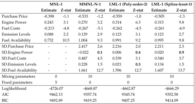
We first assumed all parameters to be random, and later incorporated fixed pa-rameters when refining this specification. Table1.2shows the parameter estimates and Z-statistic of the first specification. A very low Z-statistic of the standard devi-ation of the marginal utility of engine power in MMNL-N-1 and variants of LML-1 support preference homogeneity for power across decision-makers in the sample. The standard deviation of the marginal utility of emission levels in LML-1 (Poly-order-2) is not statistically significant (see column 7 in Table1.2), also providing evidence for further investigation.
As next steps, ASCs and fixed parameters are sequentially incorporated. The results of intermediate specifications are summarized in Table1.3. While the mean
Table 1.2: Estimation Results - All Random Parameters
MNL-1 MMNL-N-1 LML-1 (Poly-order-2) LML-1 (Spline-knot-1) Estimate Z-stat Estimate Z-stat Estimate Z-stat Estimate Z-stat
Purchase Price -0.398 -1.1 -0.533 -1.2 -0.559 -1.0 -0.505 -1.3 Engine Power 0.243 3.1 0.270 3.2 0.314 6.3 0.315 9.8 Fuel Costs -0.213 -4.8 -0.267 -5.1 -0.262 -4.5 -0.261 -4.9 Emission Levels 0.088 2.2 0.129 2.9 0.123 3.1 0.123 2.7 Fuel Availability 0.732 10.5 1.004 9.3 0.991 9.2 0.995 9.8 SD.Purchase Price - - 2.417 2.6 2.216 2.0 2.211 2.3 SD.Engine Power - - - 0.022 0.1 0.006 0.4 0.020 0.9 SD.Fuel Costs - - 0.487 4.5 0.539 3.1 0.540 3.7 SD.Emission Levels - - 0.228 1.5 0.021 0.3 0.134 1.5 SD.Fuel Availability - - 1.661 12.7 1.596 12.7 1.607 13.7 Mixing parameters 0 10 10 10 Fixed parameters 5 0 0 0 Loglikelihood -4726.07 -4668.87 -4662.87 -4666.29 AIC 9462.13 9357.74 9345.74 9352.58 BIC 9492.89 9419.25 9407.25 9414.09
of the marginal utility of emission levels is significant in MMNL-N-15, inclusion
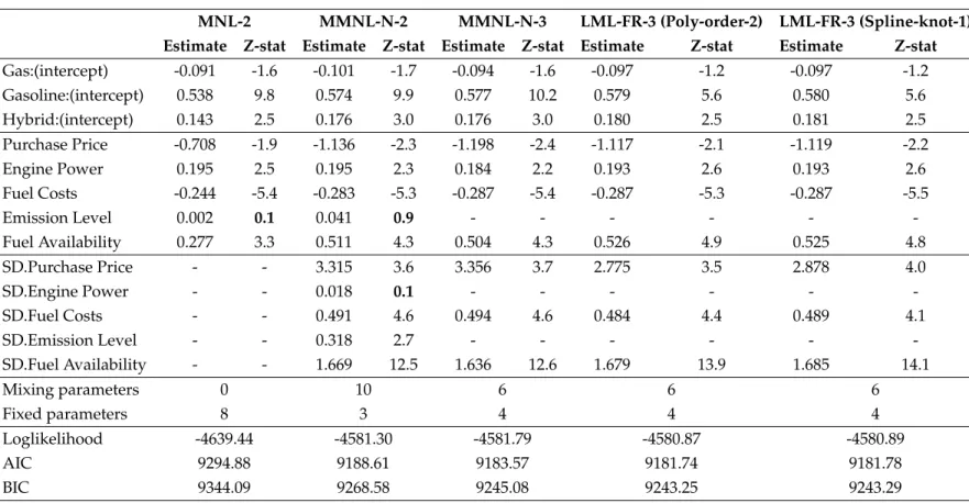
of ASCs in MNL-2 and MMNL-N-2 (see columns 2–5 in Table 1.3) results into statiscally insignificant estimates of emissions. MMNL-N-2 confirms the find-ing of MMNL-N-1 about homogeneity in preferences for engine power. Thus, specification 3 was obtained by eliminating emission levels and assuming a fixed marginal utility of engine power (see columns 6 to 11 in Table1.3).
5In MNL-1 and MMNL-N-1 specification, the significant positive correlation between
emis-sions and vehicle choice may be an artifact of not controlling for ASCs (fuel specific fixed-effects). Gasoline cars were most frequently selected (37%) and are on average dirtier than their hybrid and electric counterparts.
Table 1.3: Estimation Results - Inclusion of ASCs and Fixed Parameters
MNL-2 MMNL-N-2 MMNL-N-3 LML-FR-3 (Poly-order-2) LML-FR-3 (Spline-knot-1) Estimate Z-stat Estimate Z-stat Estimate Z-stat Estimate Z-stat Estimate Z-stat
Gas:(intercept) -0.091 -1.6 -0.101 -1.7 -0.094 -1.6 -0.097 -1.2 -0.097 -1.2 Gasoline:(intercept) 0.538 9.8 0.574 9.9 0.577 10.2 0.579 5.6 0.580 5.6 Hybrid:(intercept) 0.143 2.5 0.176 3.0 0.176 3.0 0.180 2.5 0.181 2.5 Purchase Price -0.708 -1.9 -1.136 -2.3 -1.198 -2.4 -1.117 -2.1 -1.119 -2.2 Engine Power 0.195 2.5 0.195 2.3 0.184 2.2 0.193 2.6 0.193 2.6 Fuel Costs -0.244 -5.4 -0.283 -5.3 -0.287 -5.4 -0.287 -5.3 -0.287 -5.5 Emission Level 0.002 0.1 0.041 0.9 - - - -Fuel Availability 0.277 3.3 0.511 4.3 0.504 4.3 0.526 4.9 0.525 4.8 SD.Purchase Price - - 3.315 3.6 3.356 3.7 2.775 3.5 2.878 4.0 SD.Engine Power - - 0.018 0.1 - - - -SD.Fuel Costs - - 0.491 4.6 0.494 4.6 0.484 4.4 0.489 4.1 SD.Emission Level - - 0.318 2.7 - - - -SD.Fuel Availability - - 1.669 12.5 1.636 12.6 1.679 13.9 1.685 14.1 Mixing parameters 0 10 6 6 6 Fixed parameters 8 3 4 4 4 Loglikelihood -4639.44 -4581.30 -4581.79 -4580.87 -4580.89 AIC 9294.88 9188.61 9183.57 9181.74 9181.78 BIC 9344.09 9268.58 9245.08 9243.25 9243.29 15
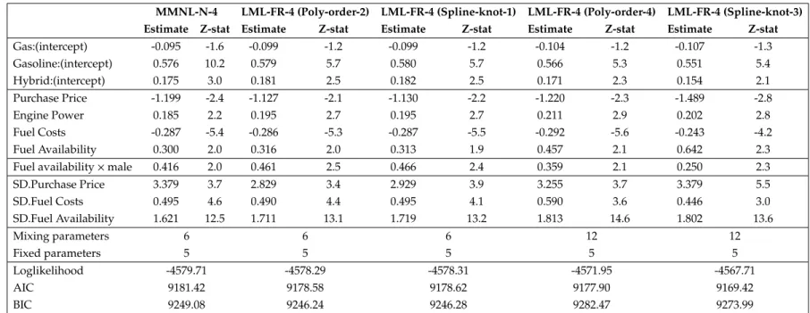
Table 1.4: Estimation Results - Final Specification
MMNL-N-4 LML-FR-4 (Poly-order-2) LML-FR-4 (Spline-knot-1) LML-FR-4 (Poly-order-4) LML-FR-4 (Spline-knot-3) Estimate Z-stat Estimate Z-stat Estimate Z-stat Estimate Z-stat Estimate Z-stat
Gas:(intercept) -0.095 -1.6 -0.099 -1.2 -0.099 -1.2 -0.104 -1.2 -0.107 -1.3 Gasoline:(intercept) 0.576 10.2 0.579 5.7 0.580 5.7 0.566 5.3 0.551 5.4 Hybrid:(intercept) 0.175 3.0 0.181 2.5 0.182 2.5 0.171 2.3 0.154 2.1 Purchase Price -1.199 -2.4 -1.127 -2.1 -1.130 -2.2 -1.220 -2.3 -1.489 -2.8 Engine Power 0.185 2.2 0.195 2.7 0.195 2.7 0.211 2.9 0.202 2.8 Fuel Costs -0.287 -5.4 -0.286 -5.3 -0.287 -5.5 -0.292 -5.6 -0.243 -4.2 Fuel Availability 0.300 2.0 0.316 2.0 0.313 1.9 0.457 2.1 0.642 2.3
Fuel availability×male 0.416 2.0 0.461 2.5 0.466 2.4 0.359 2.1 0.250 2.3
SD.Purchase Price 3.379 3.7 2.829 3.4 2.929 3.9 3.255 3.7 3.379 5.5 SD.Fuel Costs 0.495 4.6 0.490 4.4 0.495 4.1 0.590 3.6 0.446 3.0 SD.Fuel Availability 1.621 12.5 1.711 13.1 1.719 13.2 1.813 14.6 1.802 13.6 Mixing parameters 6 6 6 12 12 Fixed parameters 5 5 5 5 5 Loglikelihood -4579.71 -4578.29 -4578.31 -4571.95 -4567.71 AIC 9181.42 9178.58 9178.62 9177.90 9169.42 BIC 9249.08 9246.24 9246.28 9282.47 9273.99 16
We further sequentially explored specifications where marginal utility of alternative-specific attributes vary with socio-demographics. Table1.4 shows es-timates of the final specification that indicates gender-based statistical differences in the mean of the marginal utility of fuel availability. The model fit statistics (log-likelihood, AIC, and BIC) and resultant estimates of MMNL-N-4 are close to that of LML-FR-4 variants with the same number of parameters (see columns 2-7 in Table1.4).
The estimates indicate that the average Chinese car buyer prefers more pow-erful cars, but also likes to save on fuel costs. A dense fueling network is highly appreciated, as it guarantees the desired level of flexibility and mobility. As ex-pected, the mean of the purchase price coefficient is negative but also turns out be statistical significant, unlike the first specification with all random parameters (Table1.2).
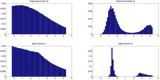
The more flexible LML-FR-4 specifications, i.e. with more parameters (see columns 8–11 in Table1.4), resulted into a higher loglikelihood at convergence but worse BIC values than that of specifications with a lower number of parameters. Thus, LML-FR with a lower number of parameters appears as preferable based on BIC.6Whereas the mean and standard deviation estimates was similar for both
specifications, more flexible specifications were able to capture multimodality of the mixing distribution (see Figures1.1, 1.2, and1.3), which cannot be retrieved with a smaller number of parameters.
6Although BIC is a standard criterion in the literature to compare different models, the use of
Figure 1.1: Histogram of Marginal Utility of Purchase Price
Figure 1.2: Histogram of Marginal Utility of Fuel Cost
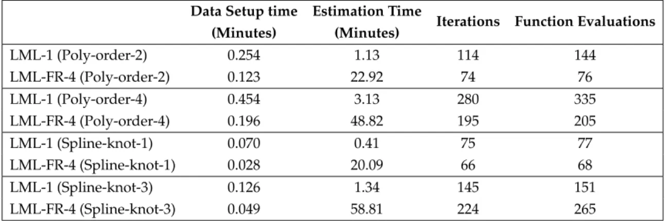
Table 1.5 compares computation time of the different LML specifications. In the standard LML model (1), data setup time is higher than that of
LML-Figure 1.3: Histogram of Marginal Utility of Fuel Availability
FR, because set up in the case of all random parameters also includes the one-time calculation ofLn(βn)(see equation 1.2). This calculation is not needed in the
LML-FR case, but we recall that the probability of the sequence of choices needs to be computed at each iteration. This iterative computation of Ln(βn) in
LML-FR-4 elevates the estimation time per iteration to 31.2 and 55.7 times (and total estimation time to 16.6 and 41.9 times) that of LML-1 for the polynomial (second order) and spline (knot 1), respectively. These ratios of estimation time remain the same for more flexible specifications. In LML-FR-4, specifying the mixing distribution with a fourth-order polynomial and three-knot spline took around 2.1 and 2.9 times that of second-order polynomial and one-knot spline, respectively.
Table 1.5: Comparing Computation Time of LML and LML-FR
Data Setup time (Minutes)
Estimation Time
(Minutes) Iterations Function Evaluations
LML-1 (Poly-order-2) 0.254 1.13 114 144 LML-FR-4 (Poly-order-2) 0.123 22.92 74 76 LML-1 (Poly-order-4) 0.454 3.13 280 335 LML-FR-4 (Poly-order-4) 0.196 48.82 195 205 LML-1 (Spline-knot-1) 0.070 0.41 75 77 LML-FR-4 (Spline-knot-1) 0.028 20.09 66 68 LML-1 (Spline-knot-3) 0.126 1.34 145 151 LML-FR-4 (Spline-knot-3) 0.049 58.81 224 265
1.4
Conclusions
The recently proposed logit-mixed logit (LML) model (Train, 2016) uses a semi-parametric representation of unobserved preference heterogeneity that is simple to implement. This chapter extends LML as derived byTrain(2016) –all parame-ters of interest assumed random– to an LML model with a combination of fixed and random parameters (LML-FR), implemented in preference space, and mo-tivated by the consideration fixed components such as alternative specific con-stants and interactions between preference parameters and socio-demographics. Whereas computational efficiency is the key feature of LML, we have shown in this chapter that the incorporation of fixed parameters considerably increases es-timation time and discussed what provokes the efficiency loss: repeated compu-tation of choice probabilities in iterative optimization. In fact, in the empirical ap-plication (stated preferences for alternative fuel vehicles by Chinese consumers; N=578, T = 6, J = 4), estimation time of the LML model with fixed and random
parameters is 20-40 times higher than that of the LML model with all parameters random. This computation time ratio depends on the sample size and can become excruciating for large sample sizes.
The higher LML-FR computation time is also a concern for hypothesis test-ing and interval estimation, because bootstrapptest-ing is the only way to derive LML standard errors7. Even if LML-FR loses computational efficiency, its flexibility is
invaluable for empirical applications. As illustrated in this study, LML-FR can re-trieve multimodality of unobserved preference heterogeneity (c.f. standard para-metric models that dominate discrete choice modeling that impose unimodality). The number of parameters and functional form of the mixing distribution, evalu-ating histogram of random parameters in several scenarios, should be considered for specification selection in addition to standard metrics such as BIC (Bansal et al., 2018a).
7If 100 bootstrap samples are taken and LML-FR estimation time for one sample is 15 times that
of the standard LML estimation time, then computation time of the LML-FR standard errors ends up being 1500 times higher than that of the LML model with all parameters random.
CHAPTER 2
MINORIZATION-MAXIMIZATION (MM) ALGORITHMS FOR SEMIPARAMETRIC LOGIT MODELS: BOTTLENECKS, EXTENSIONS,
AND COMPARISONS
2.1
Introduction
2.1.1
Background
With the increase in computation power during the last decade, the mixed multi-nomial logit (MMNL) model – a random parameter logit model with parametric and continuous heterogeneity distributions – is the most commonly used flexible discrete-choice specification (Train, 2009; McFadden and Train, 2000). The prob-lem of correctly specifying the heterogeneity (or mixing) distribution of the ran-dom parameters has received great attention (Hensher and Greene, 2003); how-ever, there is still no consensus among researchers: restricting the shape of the mixing distributions can result into wrong signs and overestimation of welfare measures. Wrong (welfare) estimates can misguide policy and marketing deci-sions (Fosgerau,2006;Cherchi and Polak,2005). To overcome the problem of pre-suming the shape of the mixing distribution, differing specifications with semi- or nonparametric mixing distributions have been proposed. Vij and Krueger(2017) andBhat and Lavieri (2017) provide a detailed review of advancements in para-metric and semiparapara-metric mixing distributions under extreme-value-distributed
(logit kernel) and normally-distributed (probit kernel) error structures. In general, estimation of these flexible1models is complex and computationally expensive.
This study focuses on estimation of two state-of-the-art semiparametric logit models, namely the logit-mixed-logit (LML) and mixture-of-normals multino-mial logit (MON-MNL) models, especially in the context of the promising perfor-mance of an alternative iterative optimization method with minimal coding, the minorization-maximization algorithm that will be introduced below, as reported for mixed logit (James,2017).
The logit-mixed-logit model (Train, 2016) generalizes many previous semi-parametric models including Bajari et al. (2007), Fosgerau and Bierlaire (2007), Train (2008), and Fox et al. (2011) (cf. Bhat, 1997). In LML, a finite parameter space is divided into a discrete multidimensional grid (cf.Train, 2008). Whereas Train(2008) considers the probability mass at each discrete point as a parameter of interest, LML reduces the number of parameters by specifying this probability using a logit link. In Monte Carlo studies, Bansal et al. (2018a) and Franceschi-nis et al.(2017) successfully tested flexibility of LML as the model could retrieve a series of continuous parametric mixing distributions (bi-modal, tri-modal, log-normal, and uniform) much better than parametric counterparts. The maximum simulated likelihood estimator (MSLE) of LML is much faster than that of para-metric models, but computation of standard errors requires bootstrapping. Fur-thermore, the computational efficiency of point estimation is lost by a factor of 15 1Model flexibility understood as the capacity to represent unobserved preference heterogeneity.
to 30 when fixed parameters are introduced (Bansal et al., 2018b), and computa-tional efficiency becomes much worse when standard errors are derived.
The mixture-of-normals multinomial logit also offers a flexible representation of unobserved preference heterogeneity. The premise of MON-MNL2 is that any
continuous distribution can be approximated to a given degree of accuracy by a discrete mixture of normals (Ferguson, 1973). Prespecifying the number of mix-ture components (or classes3) imposes a heterogeneity structure, but unlike LML
there is no need of predefining the parameter space. Resource-intensive boot-strapping to compute standard errors is not needed in MON-MNL either. In a Monte Carlo study, Fosgerau and Hess (2009) found that MON-MNL outper-formed parametric specifications in all scenarios, ranging from retrieving the most trivial uniform distribution to the most complex multimodal distribution. Keane and Wasi(2013) further supported the superiority of MON-MNL in an extensive study of 10 stated preference datasets. However, only a handful of empirical stud-ies have used MON-MNL, possibly due to the complexity of the analytical dient of the loglikelihood and covergence problems when using numerical gra-dients. For instance, Fosgerau and Hess (2009) pointed out that MSLE led into troubles for more than 2 normal components in the mixing distribution. Whereas Keane and Wasi(2013) did not explicitly mention any such estimation problem, the authors set bounds on some parameters and also imposed hard constraints on the variance-covariance matrix of each component of the mixture.
2MON-MNL was labeledMixed-Mixed LogitbyKeane and Wasi(2013) and Latent Class Mixed
Multinomial Logit model byGreene and Hensher(2013).
Among frequentist methods to estimate logit models, researches have explored iterative optimation methods. Within this class of methods, the expectation-maximization (EM) algorithm has been reported (Bhat, 1997; Cherchi and Gue-vara, 2012; Sohn, 2017) to outperform MSLE in numerical stability (i.e., less sen-sitivity to initial values), empirical identification (i.e., avoiding an invertible Hes-sian matrix), and estimation simplicity. Whereas MSLE directly maximizes the loglikelihood function using quasi-Newton methods, the simplicity of EM stems from iteratively maximizing a simpler surrogate function and update parameters while maintaining monotonic improvements in the loglikelihood (Dempster et al., 1977;McLachlan and Krishnan, 2007). Furthermore, iterative parameter updates of the EM algorithm are either closed-form or straightforward econometric prob-lems that can be solved using standard statistical packages (Train, 2008; Sohn, 2017). EM also provides a convenient parameterization of the complete-data like-lihood function without worrying about over-identification (Ruud,1991). In addi-tion to these nice statistical properties, EM also converges quickly to the neighbor-hood of the optima. However, EM is plagued by slower convergence within the optimum neighborhood (Dempster et al., 1977). In fact, the computational per-formance of EM largely hinges upon the underlying data generating process and how well EM re-characterizes the objective function. More specifically, if the com-plete data model provides much more information about the parameter than the incomplete data model, then the EM algorithm is generally slow (Meilijson,1989). Ruud(1991) suggested designing hybrid algorithms such that EM starts the max-imization process and a Newton-type algorithm finishes it. In fact, Bhat (1997)
could achieve computational efficiency and numerical stability in latent class logit estimation by shifting from EM to quasi-Newton methods when the difference in the loglikelihood of successive iterations achieved a given precision.
For some model specifications EM does not provide closed-form updates (the source of the EM benefits) for all parameters, making EM a rather slow method for estimation. For this reason, researchers have been exploring other alterna-tive estimation methods. EM is actually nested in the minorization-maximization (MM) family of iterative optimization methods (Lange et al.,2000). Note that if all iterative parameter updates in EM are closed-form (optimization-free), MM and EM are basically the same method. MM as proposed by James (2017) replaces iterative optimization of a weighted MNL model with a closed-form parameter update for a mixed logit specification with fixed and random parameters. The MM algorithm in that context was 5-8 times faster than standard EM in general, and outperformed MSLE in some panel-data settings (James,2017).
2.1.2
Research Gap and Contribution
Whereas Train (2008) proposed EM for an MON-MNL specification with all marginal-utility parameters being random, no such algorithm exists for LML. Even if EM for the all-random-parameters MON-MNL requires just computing sums and multiplications to iteratively update parameters, it has not been further used in practice. Moreover, the consideration of some parameters being fixed may
play against simplicity of estimation of flexible discrete choice models, as noted for EM in the mixed logit work ofJames(2017).
In addition to focus on a general utility specification with fixed and random parameters due to the implementation challenges that may appear in iterative op-timization methods, we argue that inclusion of fixed parameters is important for empirical reasons.Ruud(1996) suggests to hold at least one coefficient fixed in the mixed logit model because a specification with all random coefficients is almost unidentified empirically. Moreover,Train(2009) recommends to keep alternative-specific constants fixed due to the same reason. Empirical identification also re-stricts parameters to be fixed in the case of interactions with sociodemographics that represent taste variation with respect to a (random) parameter.4 Finally,
will-ingness to pay for a specific covariate may not vary across the population and thus the estimated parameter may be just non-random.
The main contribution of this chapter is to derive MM algorithms (including standard EM) to estimate semiparametric logit models under general utility spec-ifications, identify key bottlenecks in the MM algorithm with all closed-form up-dates, propose a faster-MM algorithm and illustrate its parallel implementation, and finally compare the different variants of EM and MM algorithms with quasi-Newton methods in a Monte Carlo study and an empirical study. Since our con-tribution is fourfold, details are discussed below.
4Consider an indicator variable for malesD
maleand a taste-variation-specification of the type
(βik+βmaleDmale)xik. Whileβikcan be considered random, for empirical identificationβmalewould
Thefirst contributionof this study is to derive standard EM for LML (cf. Bhat, 1997, for a latent class logit model) and to extend EM for MON-MNL under more general utility specifications. Even though the proposed EM algorithm for LML and MON-MNL can be implemented easily in any standard statistical package, we show that – just as in mixed logit, although the equations are different – EM in-trinsically involves computationally burdensome optimizations of weighted MNL (WMNL) loglikelihood functions (see sections 2.2.2 and 2.3.2). Whereas the EM algorithm for LML involves iterative estimation of two WMNL models, we show that EM for MON-MNL requires as many WMNL loglikelihood maximizations at each iteration as the number of mixture components. We also show that these resource-intensive computations may even rule out EM as a feasible option to es-timate semiparametric logit models in practice.
Given the computational performance issues of EM discussed above, the sec-ond contributionof this study is to derive MM for both LML and MON-MNL mod-els. We discuss and illustrate several advantages of MM over EM in section2.4. In particular, optimization-free (closed-form) parameter updates in MM makes it attractive since it can be easily integrated into flexible5 estimation software.
Fur-thermore MM just requires storage of sufficient statistics, and we thus demon-strate how parallel computation can result into 80% reduction in estimation time.6
Although we were first expecting to see computational efficiency improvements 5Code flexibility is understood as the capacity of software to allow the analyst to directly specify
the desired loglikelihood, avoiding restrictions such as only linear-in-parameter utility specifica-tions.
6The EM algorithm can also be parallelized, but storage and communication of large
such as the ones observed byJames(2017) for mixed logit, MM computation time for LML was disappointing even after parallel estimation. What happens is that the MM algorithm’s lower bound approximation is very poor if the WMNL model has a large choice set (seeBöhning and Lindsay, 1988), which is by construction exactly the case of LML: the number of “alternatives” in the WMNL update is equal to the number of random draws (in the order of 1000s) taken from the mul-tidimensional grid that represents the parameter space. In fact, through a Monte Carlo study, we found that MM for MON-MNL and even the parametric mixed logit model also encounter computational failure for a large choice set. This issue is critical because large choice sets are often encountered in revealed preference studies, precisely in applied work where alternative estimation methods such as EM and MM are needed (von Haefen and Domanski,2018).
The third contribution of this study is the identification of bottlenecks in the implementation of MM and provide improvements. Following the method sug-gested by Böhning and Lindsay (1988), we propose a faster-MM algorithm in which the embedded step-size is corrected. The proposed faster-MM algorithm is general and useful to improve the lower-bound approximation of any WMNL loglikelihood while keeping the simplicity of MM. However, the computational gains largely depend on the cardinality of the choice set. For example, faster-MM could reduce computation time of MM for an LML model by a factor of around 100 due to a very high (order of 1000s) cardinality of the choice set of the iterative WMNL.
The fourth contribution of this study is to highlight shortcomings and advan-tages of the existing and proposed estimation methods using an extensive Monte Carlo study and an empirical application to estimate consumer’s willingness to adopt electric motorcycles in Solo, Indonesia.
The remaining of the chapter is organized as follows: sections 2 and 3 derive the iterative-optimization estimation algorithms for LML and MON-MNL; section 4 draws insights from the derived procedures; section 5 describes the Monte Carlo studies and discusses the findings; section 6 focuses on the empirical study; and conclusions are detailed in section 7.
2.2
Iterative Optimization Methods to Estimate the Logit Mixed
Logit (LML) Model
2.2.1
Logit-Mixed Logit (LML)
Let N be the number of decision-makers in a sample where each agent faces T
choice situations and chooses a utility-maximizing alternative from a set of J al-ternatives. The conditional indirect utility of decision-makerifrom making choice
jin choice situationtis:
wherei ∈ {1, . . . ,N}, j ∈ {1, . . . ,J}, andt ∈ {1, . . . ,T}. We consider the general case
in which attributes can be partitioned between those having fixed parameters (x) and those with random parameters (z) with a general continuous heterogeneity distribution.7 The attribute vector x
it jthus has a fixed preference parameter
vec-tor α, whereas zit j has a random, individual-specific preference vector βi. The
preference shockεit j is independent across individuals, choices and time, and is
identically distributed Type-I Extreme Value. Thus, the probability of choosing alternative jby individualiin choice situationt, conditional onβi, has a logit link:
Pit j(α,βi)= expxT it jα+ z T it jβi PJ k=1exp xT itkα+z T itkβi . (2.2)
If individual i chooses alternative j in choice situation t, one can define the choice indicatordit j= I(j chosen|i,t). For the sequence of choices made by
individ-uali, the conditional likelihoodLi(α|βi)is: Li(α|βi)= T Y t=1 J Y j=1 [Pit j(α,βi)]dit j. (2.3)
In the LML model, preferences variations are represented using a discrete mix-ing distribution over a finite support setS. The probability of the randomβibeing
equal to a specific value βir is represented by the following logit link (hence the
logit-mixed logit name proposed byTrain,2016):
wi(βi =βir|φ)= expy(βir)Tφ P s∈S exp (y(βis)Tφ) , (2.4)
7As discussed in the introduction, the consideration of a combination of fixed and random
parameters not only is empirically justified but also offers estimation challenges that need to be addressed.
whereφis a vector of parameters andy(βr)is a vector-valued function (e.g. spline,
step, or polynomial function) that captures the shape of the mixing distribution. If ψ = {α,φ} summarizes the parameters of interest, the unconditional likeli-hoodPi(ψ)of agentiis:
Pi(ψ)=X r∈S
Li(α,βir)wi(βir|φ), (2.5)
and the corresponding loglilkelihood`(ψ)of the sample is: `(ψ)= N X i=1 ln X r∈S Li(α,βir)wi(βir|φ) . (2.6)
Maximizing the loglikelihood becomes intractable in practice if the entire sup-port set S is used. Therefore, a large subset of parameter vectors (for example, 2000 vectors) for each decision-maker is sampled from the support set (see sec-tions2.5.1and2.6for details) to derive the maximum simulated likelihood estima-tor of the model. The standard errors of the parameters of interest are calculated through bootstrapping.
2.2.2
LML Estimation using the EM Algorithm
The EM algorithm was originally developed to deal with missing data (Dempster et al., 1977). Since several loglikelihood maximization problems can be viewed as a missing data problem, the EM algorithm has been widely used in different disciplines (McLachlan and Krishnan, 2007). The EM algorithm is a two-step –
the expectation (E) step and the maximization (M) step – iterative procedure. In the E-step, data are completed (in a probabilistic sense) conditional on previous iteration parameters. In the M-step, parameters are optimized conditional on the completed data. The algorithm terminates when difference in parameter estimates of two consecutive iterations is very small.
Bhat (1997) first introduced the EM algorithm into the discrete choice litera-ture for the estimation of models with endogenous segmentation or latent classes. Since LML generalizes the latent class logit model, the missing data for the EM algorithm in LML estimation are the parameters of each agent in each draw (βir)
just as originally suggested in Bhat (1997). As a result, the M-step Q(ψ|ψm) and
E-step of the EM algorithm for LML model are:
E-step: hir(βir|ψm)= Li(αm,βir)wi(βir|φm) P r∈SLi(αm,βir)wi(βir|φm) = Li(αm,βir)wi(βir|φm) Pi(ψm) , (2.7) M-step: Q(ψ|ψm)= N X i=1 X r∈S hir(βir|ψm) ln Li(α,βir)wi(βir|φ) , (2.8)
wherehir(βir|ψm)are weights that are computed at each iteration (ψm+1) using the
previous iteration (ψm). The M-step surrogate function is additive separable in the
fixed parameters (α) and the parameters defining the shape of the mixing distri-bution (φ): Q(ψ|ψm)= N X i=1 X r∈S hir(βir|ψm) ln(Li(α,βir))+ N X i=1 X r∈S hir(βir|ψm) ln(wi(βir|φ)). (2.9)
As expected, optimizing these two independent functions separately is much easier than the joint maximization problem. The EM update equations are:
Q(α|ψm)= N X i=1 X r∈S hir(βir|ψm)ln(Li(α,βir)) =⇒ αm+1 =argmax α Q(α |ψm) (2.10) Q(φ|ψm)= N X i=1 X r∈S hir(βir|ψm)ln(wi(βir|φ)) =⇒ φm+1 =argmax φ Q(φ |ψm), (2.11) whereQ(α|ψm
)represents a weighted multinomial logit loglikelihood (with fixed utility weightsα) andQ(φ|ψm)
represents a very similar expression to the weighted multinomial logit loglikelihood (with characteristics y(βir) and weightsφ). If all
utility parameters are random, the algorithm remains the same after removing equation2.10to update the fixed parameters. The complete EM algorithm for the LML model is summarized below:
2.2.3
LML Estimation using the MM Algorithm
In the EM algorithm for LML, numerical maximization ofQ(α|ψm)and Q(φ|ψm)at
each iteration can be computationally burdensome. Inspired in the work byJames (2017) for mixed logit, we propose the use of the minorization-maximization (MM) algorithm (Lange et al., 2000), where closed-form surrogate functions [Qe(α|ψm),Qe(φ|ψm)] create closed-form updates of the parameters (ψ= {α,φ})
Algorithm 1:EM for the LML Model Initialization
For eachi, drawβir,r =1, . . . ,R(e.g.,R= 2000), from the support setS;
Compute y(βir)using sieve functions such as spline;
Initialize parametersm=0: ψ0 = {α0,φ0} whilekψm+1−ψmk
∞ <Tol.do
Step 1:Calculation of the weight [hir(βir|ψm)];
CalculatePit j(αm,β
ir)for eachβirusing Eq. 2.2;
CalculateLi(αm,βir)for eachiand for eachβir using Eq.2.3;
Calculatewi(βir|φm)for eachiand for eachβirusing Eq. 2.4;
Calculatehir(βir|ψm)for eachβirusing Eq. 2.7; Step 2:Update parameters;
Updateαm+1using Eq. 2.10;
Updateφm+1 using Eq.2.11; end
The new surrogate functions are derived using a quadratic lower bound ap-proximation of the Hessian.8 This approximation can be used to reduce the
op-timization burden of any EM algorithm which iteratively optimizes the loglikeli-hood of a weighted MNL model.9
Updatingφ
The new surrogate function to updateφusing the approximation is:
e
Q(φ|ψm)= Q(φm|ψm)+(φ−φm)Tgmφ + (φ
−φm)TBm
φ(φ−φm)
2 , (2.12)
8A function can be bounded below by a quadratic approximation if there exists a global lower
bound to the second derivative (Böhning and Lindsay,1988). In fact,James(2017) proposed the MM algorithm to estimate the MMNL model exploiting the same idea.
9However, MM estimation time can be higher than EM estimation time, or vice versa,
wheregmφ = ∂Q(φ|ψ m) ∂φ φ=φm and Bmφ ≤ ∂ 2Q(φ|ψm) ∂φ2 . Thus, φm+1 =φm− [Bmφ]−1gmφ. (2.13)
This new update equation ofφis a single Newton step that only requires the gradient and lower bound on the Hessian of the EM surrogate function Q(φ|ψm)
, which are computed as follows (seeBöhning and Lindsay,1988, for details):
gmφ = ∂Q(φ|ψ m) ∂φ φ=φm = N X i=1 X r∈S hir(βir|ψm) y(βir)− X v∈S [y(βiv)wi(βiv|φm)] (2.14) Hφm= ∂ 2Q(φ|ψm) ∂φ2 φ=φm = − N X i=1 X r∈S hir(βir|ψm) h X v∈S y(βiv)[y(βiv)]Twi(βiv|φm)− X v∈S y(βiv)wi(βiv|φm) X v∈S [y(βiv)]Twi(βiv|φm) i (2.15) Bmφ = −1 2 N X i=1 X r∈S hir(βir|ψm) h X v∈S y(βiv)[y(βiv)]T − 1 R X v∈S y(βiv) X v∈S [y(βiv)]T i (2.16) X r∈S hir(βir|ψm) = 1 =⇒ (2.17) Bmφ = Bφ = −1 2 N X i=1 h X v∈S y(βiv)[y(βiv)]T− 1 R X v∈S y(βiv) X v∈S [y(βiv)]T i . Updatingα
Similarly we take lower bound approximation ofQ(α|ψm)(see equation2.12) and
the update equation forαis:
αm+1 =αm−