Beyond Contiguity: The Role of Temporal Distributions
and Predictability in Human Causal Learning
A dissertation submitted to the School of Psychology, Cardiff University, in partial fulfilment of the requirements for the degree of
Doctor of Philosophy September, 2011 by
James Greville
School of Psychology Cardiff University Tower Building Park Place CF10 3AT Cardiff, UKAbstract
Most contemporary theories of causal learning identify three primary cues to causality; temporal order, contingency and contiguity. It is well-established in the literature that a lack of temporal contiguity – a delay between cause and effect – can have an adverse effect on causal induction. However research has tended to focus almost exclusively on the extent of delay while ignoring the potential influence of delay variability. This thesis aimed to address this oversight.
Since humans tend to experience causal relations repeatedly over time, we accordingly experience multiple cause-effect intervals. If intervals are constant, it becomes possible to predict when the effect will occur following the cause. Fixed delays thus confer temporal predictability, which may contribute to successful causal inference by creating an impression of a stable underlying mechanism. Five experiments confirmed the facilitatory effect of predictability in instrumental causal learning. Two experiments involving a different aspect of causal judgment found no effects of interval variability, but two further experiments demonstrated that predictability facilitates elemental causal induction from observation. These results directly conflict with findings from studies of animal conditioning, where preference for variable- interval reinforcement is routinely exhibited, and a simple associative account struggles to explain this disparity. However both a temporal coding associative account, and higher-level cognitive perspectives such as Bayesian structural inference, are compatible with these findings. Overall, this thesis indicates that causal learning involves processes above and beyond simple associations.
Preface
This thesis was completed at the School of Psychology, Cardiff University, under the supervision of Dr. Marc Buehner, 2007-2011.
Parts of the empirical work in Chapter 3, specifically experiments 1, 2B and 3, were published in the article: Greville, W. J., & Buehner, M. J. (2010) Temporal Predictability Facilitates Causal
Learning. Journal of Experimental Psychology: General, 139(4), 756–771. Other work
undertaken during this period of study, but not presented in this thesis, is currently being revised
for publication in Memory & Cognition.
An overview of this research was presented at the following conferences:
BPS Cognitive Section Annual Conference, September 2009: University of Hertfordshire, UK; 1st joint meeting of EPS and SEPEX: April 2010, Granada, Spain; 36th Annual Convention of the Association for Behavior Analysis: June 2010, San Antonio, Texas; BPS Cognitive Section Annual Conference, September 2010: Cardiff University, UK.
This research was supported by a grant from the Engineering and Physical Sciences Research Council (EPSRC).
Acknowledgements
Firstly, immense thanks are due to my supervisor Marc Buehner. His careful guidance struck just the right balance between giving me the freedom to develop my own interests whilst still keeping me focused. I will always be very grateful for his continual encouragement along an often arduous but ultimately enjoyable journey.
I thank Cardiff University and the EPSRC for generously funding my research.
I would also like to thank my friends and collaborators at Cardiff University, in particular my second supervisor Mark Johansen, Adam Cassar, Sindhuja Sankaran, and Laurel Evans.
I thank Anthonia for countering my melancholia with her warmth and vivacity.
Finally I would like to thank my family and especially my sister, Katharine, and my parents, David and Maureen, for their enduring love and support.
Dedication
This thesis is dedicated to the memory of three dearly missed people that sadly departed during the past three years:
To my grandpa, Norman Gordon, a kind and caring man of true integrity, who proudly served his country and who loved and was loved by his family.
To my friend, Quirine C harlton-Robbins, whose bravery in the face of adversity was incredible and whose cheer and generosity is missed by all those who knew her.
Finally to Christopher Douglas Brown, one of my oldest and dearest friends, who genuinely inspired me with his courage and determination to follow his own path in his own way, and showed that richness of experience rather than accumulation of years is the true measure of life.
Table of Contents
ABSTRACT ...iii
PREFACE...iii
ACKNOW LEDG EMENTS AND DEDICATION...iv
LIST O F FIGURES ...x
LIST O F TABLES ...x
CHAP TER 1 – CURRENT P ERSP ECTIVES ON CAUSAL LEARNING ...1
1.1CAU SALIT Y AND CAUSAL LEARNING –A BRIEF INTRODUCTION...1
1.2THE CENTRAL P ROBLEM FOR CAUSAL LEARNING...1
1.3PLAN OF THE THESIS...3
1.4HUME’S CUES T O CAUSALIT Y...4
1.4.1 Temporal Order...4
1.4.2 Contingency...4
1.4.3 Contiguity ...6
1.5THEORIES OF CAUSAL LEARNING...9
1.5.1 Conditioning and Associative Learning Theory ... 10
1.5.1.1 The Rescorla-Wagner M odel... 11
1.5.1.2 The Role of Time from an Associative Persp ective ... 13
1.5.1.3 Difficulties for an Associative Account of Causality Judgment... 15
1.5.2 Causal Mechanism and Power Theories... 16
1.5.2.1 The Power PC Theory... 17
1.5.2.2 The Role of Time from Covar iation Persp ectives ... 18
1.5.3 Causal Models and Structure Theories... 20
1.5.3.1 Causal M odel Theory... 21
1.5.3.2 Bay esian Structure Learnin g ... 23
1.5.3.3 Causal Sup port... 24
1.5.3.4 A Bayesian Persp ective on Contiguity... 25
1.5CHAPT ER SUMMARY...27
CHAP TER 2 – TH E P OTENTIAL RO LE O F TEMPO RAL PREDICTAB ILITY IN CAUSAL LEARNING ... 30
2.1INT RODUCING TEMPORAL PREDICTABILITY...30
2.2.THE TEMP ORAL PREDICTABILITY HYPOTHESIS...32
2.3PREVIOUS EMPIRICAL RESEARCH ON PREDICTABILITY...34
2.4ANIMAL PREFERENCE FOR VARIABLE REINFORCEMENT...35
2.5THEORETICAL PERSPECTIVES ON PREDICTABILITY...37
2.5.1 An Associative Analysis of Temporal Predictability... 37
2.5.2 The Attribution Shift Hypothesis... 41
2.5.3 Bayesian Models ... 42
2.6CHAPT ER SUMMARY...44
CHAP TER 3 – TH E RO LE O F TEMP O RAL PREDICTABILITY IN INSTRUMENTAL CAUS AL LEARNING... 46
3.1OVERVIEW AND INTRODUCTION...46
3.2EXP ERIMENT 1...47
3.2.1 Method ... 49
3.2.1.1 Particip ants... 49
3.2.1.2 Design ... 49
3.2.1.3 App aratus, Materials and Procedure ... 51
3.2.2.1 Causal Judgments... 52
3.2.2.2 Instrumental Behaviour and Outcome Patterns ... 55
3.2.3 Discussion ... 57
3.3EXP ERIMENT 2A ...58
3.3.1 Method ... 59
3.3.1.1 Particip ants... 59
3.3.1.2 Design ... 60
3.3.1.3 App aratus, materials & p rocedure ... 61
3.3.2 Results & Discussion... 61
3.3.2.1 Causal Ratings... 61 3.3.2.2 Behavioural Data... 63 3.2.3 Discussion ... 63 3.3EXP ERIMENT 2B...64 3.3.1 Method ... 66 3.3.1.1 Particip ants... 66 3.3.1.2 Design ... 66
3.3.1.3 App aratus, Materials & Procedure... 67
3.3.2 Results... 67
3.3.2.1 Causal Ratings... 67
3.3.2.2 Instrumental Behaviour and Outcome Patterns ... 68
3.3.3 Discussion ... 69
3.4EXP ERIMENT 3...71
3.4.1 Method ... 72
3.4.1.1 Particip ants... 72
3.4.1.2 Design ... 72
3.4.1.3 App aratus, materials & p rocedure ... 73
3.4.2 Results... 73
3.4.2.1 Causal Ratings... 73
3.4.2.2 Instrumental Behaviour and Outcome Patterns ... 74
3.4.3 Discussion ... 75
3.5EXP ERIMENT 4...76
3.5.1 Overview of exp eriment... 77
3.5.2 Predictions... 78
3.5.3 Method ... 78
3.5.3.1 Particip ants... 78
3.5.3.2 Design ... 78
3.5.3.3 App aratus& M aterials ... 79
3.5.3.4 Procedure ... 79
3.5.4 Results... 79
3.5.4.1 Causal Judgments... 79
3.5.4.2 Instrumental Behaviour and Outcome Patterns ... 80
3.5.5 Discussion ... 81
CHAPTER SUMMARY...83
CHAP TER 4 – TH E RO LE O F TEMP O RAL PREDICTABILITY IN OBS ERVATIO NAL CAUS AL LEARNING... 84
4.1PARALLELS AND DISP ARITIES BETWEEN CLASSICAL AND INST RUMENTAL CONDITIONING...85
4.2DIST INGUISHING INTERVENTION AND OBSERVATION...86
4.3EXI ST ING EVIDENCE –YOUNG &NGUYEN,2009 ...88
4.3.1 An alternative to the predictability hypothesis – The temporal proximity account... 90
4.3.2 The video game context... 92
4.4EXP ERIMENT 4A ...92
4.4.1 Predictions ... 94
4.4.2 Speed-Accuracy Tradeoff... 94
4.4.3 Method ... 95
4.4.3.1 Particip ants and App aratus... 95
4.4.3.3 Design and Materials ... 96
4.4.3.4 Procedure ... 97
4.4.4 Results... 99
4.4.4.1 Sp eed-Accuracy Tradeoff ... 100
4.4.4.3 Accuracy ... 102 4.4.5 Discussion ...104 4.5EXP ERIMENT 5B...108 4.5.1 Method ...109 4.5.1.1 Particip ants... 109 4.5.1.2 Design ... 109
4.5.1.3 App aratus & M aterials ... 110
4.5.1.4 Procedure ... 110 4.5.2 Results...111 4.5.2.1 Samplin g Time ... 112 4.5.2.2 Accuracy ... 113 4.5.3 Discussion ...114 4.5.3.1 A Sp eed-Accuracy Violation ... 114
4.5.3.2 Failure to find support for p redictability... 115
4.5.3.3 Temporal order violations may reveal the true cause ... 117
4.5.3.4 Alternative App lications ... 119
4.5.3.5 “Back to Basics” ... 119
4.6EXP ERIMENT 6A ...121
4.6.1 An Observational Analogue of the Elemental Causal Judgment Task ...122
4.6.2 Method ...124
4.6.2.1 Particip ants... 124
4.6.2.2 Design ... 124
4.6.2.3 App aratus, Materials and Procedure ... 124
4.6.3 Results...126
4.6.3.1 Causal Ratings... 126
4.6.3.2 Cue and outcome patterns... 127
4.6.4 Discussion ...130
4.7EXP ERIMENT 6B...134
4.7.1 Method ...134
4.7.1.1 Particip ants... 134
4.7.1.3 App aratus, Materials & Procedure... 135
4.7.2 Results...135
4.7.2.1 Causal Ratings... 135
4.7.2.2 Cue and outcome patterns... 136
4.7.3 Discussion ... 137
4.8CHAPT ER SUMMARY...140
CHAP TER 5 – GENERAL DISCUSSION AND CO NCLUSIONS ...141
5.1BRIEF SYNOP SIS OF EXPERIMENTS...141
5.2TEMP ORAL PREDICTABILITY FACILIT ATES ELEMENTAL CAUSAL INDUCTION...142
5.3AN ASSOCIATIVE ANALYSIS OF TEMPORAL PREDICTABILITY...144
5.3.1 Delay Discounting...145
5.3.2 The Temporal Coding Hypothesis...148
5.4.A CONTINGENCY-BASED PERSPECTIVE ON P REDICTABILITY...150
5.4.1 Attribution Aide or Cognitive Component?...152
5.5ABAYESIAN ACCOUNT OF P REDICT ABILITY...152
5.6ANOVEL APPROACH –TEMP ORAL EXPECT ANCY THEORY...153
5.7MET HODOLOGICAL CONCERNS...156
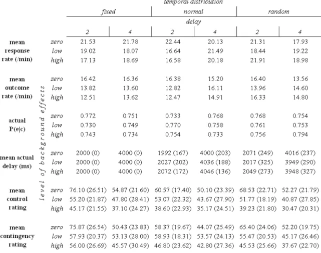
5.7.1 Interactions of Predictability with Delay Extent and Background Effects...157
5.8FUT URE DIRECTIONS...158
5.9CONCLUSIONS...160
List of Figures
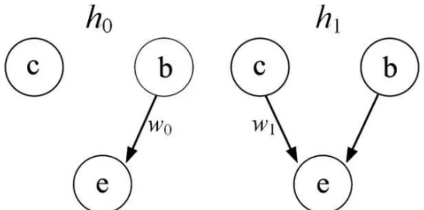
Figure 1.1: Standard 2×2 contingency matrix, showing the four possible combinations of cause and effect occurrence and non-occurrence...6 Figure 1.2: The effect of attribution shift in parsing an event stream with a specific timeframe
assumed : c e intervals that are longer than the temporal window simultaneously decrease
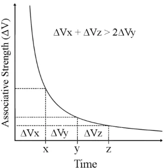
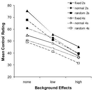
impressions of P(e|c) and P(¬e|¬c) while increasing impressions of P(e|¬c) and P(¬e|c). 19 Figure 1.3: Directed acyclic graph representing causal influence of X on Y...20 Figure 1.4: Directed acyclic graphs representing the two basic hypotheses that are compared in elemental causal induction...24 Figure 2.1: Potential differences in accrued associative strength between fixed- interval and variable-interval conditions according to a hyperbola- like discounting function of delayed events. ...40 Figure 3.1: Diagram representing the three types of temporal distribution applied in Experiment 1 at the two levels of mean delay. ...51 Figure 3.2: Mean Control Ratings for all conditions in Experiment 1 as a function of background effects. Filled and unfilled symbols refer to mean delays of 2s and 4s respectively. Delay
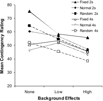
variability is noted by different symbol and line styles. Error bars are omitted for clarity. .53 Figure 3.3: Mean Contingency Ratings for all conditions in Experiment 1 as a function of background effects. Filled and unfilled symbols refer to mean delays of 2s and 4s respectively. Delay variability is noted by different symbol and line styles. Error bars are omitted for clarity. ...54 Figure 3.4: Diagram illustrating the combination of the levels Delay and Range to produce the six experimental conditions in Experiment 2A...60 Figure 3.5: Mean Causal Ratings from Experiment 2A as a function of temporal interval range. Different symbol and line styles represent different delays. Error bars show standard errors.62
Figure 3.6: Mean Causal Ratings from Experiment 2B as a function of interval range. Filled and unfilled symbols refer to master and yoked conditions respectively. Mean delays are noted by different symbol and line styles. ...68 Figure 3.7: Mean Causal Ratings from Experiment 3 as a function of interval range. Filled and unfilled symbols refer to 2 and 4 minutes training respectively. Mean delays are noted by different symbol and line styles. ...74 Figure 3.8: Mean causal ratings from Experiment 4 as a function of P(e|c). Filled and unfilled symbols refer to fixed and variable delays respectively. ...80 Figure 4.1:Screen shot of the stimuli used in Experiments 5A and 5B...98 Figure 4.1: Scatter plot showing participants’ mean percentage accuracy as a function of their mean log sampling time across all nine conditions in Experiment 5A. ...101 Figure 4.2: Mean log sampling time as a function of interval variability for all nine conditions in Experiment 5A. Different symbol and line styles denote different mean delays. Error bars show standard errors...102 Figure 4.3: Hypothetical causal model of the independent and dependent variables in Experiment 5A. Nodes represent variable and arrows represent causal influence...103 Figure 4.4: Mean percentage accuracy as a function of delay variability for all nine conditions in Experiment 5A. Different symbol and line style refer to different mean delays. Error bars are omitted due to the dichotomous nature of the dependent measure. ...104 Figure 4.5: Scatter plot showing participants’ mean percentage accuracy as a function of their mean log sampling time across all nine conditions in Experiment 5B. ...111 Figure 4.6: Mean log sampling time as a function of interval variability for all nine conditions in Experiment 5B. Different symbol and line styles denote different mean delays...112 Figure 4.7: Mean percentage accuracy as a function of interval variability for all nine conditions in Experiment 5B. Different symbol and line styles denote different mean delays. ...113
Figure 4.8: Mean causal ratings as a function of temporal interval range for all six conditions in Experiment 6A. Different symbol and line styles denote different mean delays. ...127 Figure 4.9: Mean causal ratings for Experiment 6B as a function of temporal interval range. Different symbol and line styles denote different mean delays. Error bars show standard errors. ...137
List of Tables
Table 3.1: Behavioural Data for Experiment 1. Standard deviations are given in parentheses. ...56 Table 3.2: Behavioural Data for Experiment 2A. Standard deviations are given in parentheses. ...62 Table 3.3: Behavioural Data for Experiment 2B. Standard deviations are given in parentheses. ...69 Table 3.4: Behavioural Data for Experiment 3. Standard deviations are given in parentheses. ...75 Table 3.5: Behavioural Data for Experiment 4. Standard deviations are given in parentheses. ...81 Table 4.1: Behavioural data for Experiment 6A. Standard deviations are given in parentheses. ...128 Table 4.2: Behavioural data for Experiment 6B. Standard deviations are given in parentheses. ...138
Chapter 1 – Current Perspectives on Causal Learning
1.1 Causality and Causal Learning – A brief introduction
The study of causality has a long and rich history in both philosophy and psychology. In essence, causality is understood as the relationship between one event or entity, the cause, and another event or entity, the effect, such that the second is recognized to be a consequence of the first. In other words, causes produce or generate effects. Causal learning, in the simplest sense, is how we come to learn that one thing causes another.
An expanded and more precise definition of causality acknowledges that causes may be either deterministic, where the effect necessarily follows from the cause, or probabilistic, where the cause alters the likelihood of the effect. Furthermore, causes may be generative, producing or increasing the probability of occurrence of an outcome, or preventative, inhibiting an outcome that would otherwise have occurred. Causality then may be seen as the underlying laws that govern systematic relations between events.
Multiple relationships between multiple entities or events may exist within a given system. For example, a fire may produce smoke and heat, both of which are common effects, while the fire itself may have resulted from natural causes (such as a bolt of lightning) or from deliberate human action, both of which may be regarded as common causes (or parents). Such an interconnected series of events is known as a causal network (Pearl, 2000). Causal learning may thus be more broadly defined as the process by which we construct and represent causal relations and networks, and how we use this information in thinking, reasoning, judgment and decision- making. The research presented within this thesis however focuses on the former, more fundamental question of causal learning – how do humans learn that one thing causes another?
1.2 The central problem for causal learning
The ability to learn enables us to adapt to our environment and, ultimately, to survive. If learning has evolved as an adaptive mechanism, it is natural that the content of learning should reflect relations that actually exist in the universe (Shanks, 1995). Causal learning endows us with the capacity to create representations that mirror the causal structure of our surrounding environment. Creating such representations allows us to
understand how and why events occur, to predict the occurrence of future events, and to intervene on the world and control our environment, directing our behaviour to evoke desired consequences and achieve goals. Causal learning is thus a core cognitive capacity and a crucial adaptive mechanism. The central question for learning theorists interested in causality is how such knowledge is acquired.
Seeking an answer to this question has been a preoccupation of scholars throughout the ages. Yet, this may, to the uninitiated, seem somewhat surprising. When asked “how do you learn that one thing causes another?” an immediate answer may spring to mind such as “I see it happen and so I know how it works” (Schlottmann, 1999). One might then be puzzled as to why this question has provided such a dilemma when the answer seems so intuitively obvious. For example, when one kicks a ball, the causal connection between so doing and the subsequent motion of the ball seems immediately apparent. Indeed, it has been argued that such events involving physical collision of objects or “launching” (Michotte, 1946/1963) may indeed give rise to direct causal perception (for an overview see Scholl & Tremoulet, 2000).
Consider however some alternative examples. When one practices a skill such as learning a musical instrument, there is typically a causal understanding that continued practice will lead to improved performance. However we cannot directly see the physiological changes to the neurons in the brain and muscle fibres in the body that practice confers to improve the co-ordination and dexterity of the individual. Nor can the cellular changes be observed when, for instance, a pathogen invades our body and causes illness, or a drug is taken to treat that illness and eliminate the pathogen from our system. How then, have we come to learn causal relations such as that microscopic pathogens cause illness and that certain drugs will eradicate these unwanted visitors, or that one can develop a skill through practice?
Such unobservable causal relations need not always involve biological processes. Hanging a wet cloth outside on a sunny day, for instance, will cause the cloth to dry, and we may well be able to observe the cloth becoming drier, if we have nothing better to do. What we cannot see however, is the mechanism involved, the transfer of energy, the water molecules becoming more excited and eventually changing state from liquid to vapour as they evaporate from the cloth. Moreover, we cannot directly perceive the laws of physics
governing the behaviour of molecules, such as in the evaporation of water, which ultimately underpin this process. Such causal laws or relations are not entities in themselves and are therefore imperceptible; we cannot see (nor hear, touch, smell or taste) a causal law. If such laws are unobservable, then how can we ever become aware of them?
Although philosophical concerns regarding causality extend as far back as the days of Aristotle, it was the Scottish empiricist David Hume (1711-1776) that first formalized and addressed the “riddle of induction” that is exemplified by such scenarios as described above. Hume reasoned that since our sensory modalities are not attuned to the detection of causality per se, the existence of causal relations can only be inferred from the observable evidence that is accessible to us (Hume, 1739/1888). Causal learning is therefore often referred to also as causal inference or induction. It follows then that representations of causal relations must be constructed on the basis of the sensory input we receive from the world around us. Hume proposed that there are crucial ‘cues to causality’ that underpin such representations, and identified the most important determinants as 1) temporal order – causes must precede their effects; 2) contingency – effects must repeatedly and reliably follow their causes; and 3) contiguity – causes and effects must be closely connected in space and time.
These statistical and temporal relations between events form the bedrock of nearly all theories of causal learning. The primary goal of this thesis is to address the possibility of an additional cue, namely temporal predictability, contributing to the process of causal inference. At this point then, it seems appropriate to provide a brief overview of the thesis, and outline how this question shall be approached.
1.3 Plan of the thesis
The remainder of this chapter will firstly explore in more detail each of the cues to causality as suggested by Hume, and the role each is considered to play in causal learning. Following this, I shall briefly introduce three broad theories of causal learning, each of which has its own particular interpretation of how humans and other agents use such cues to learn about causal relations. This background is necessary for the eventual evaluation of the empirical results that will be presented further on. C hapter 2 then fully introduces this concept of temporal predictability and outlines how such a feature might be a factor in
causal learning. It is then considered how each of the theories of causal learning introduced in Chapter 1 might accommodate any effects of this potential cue of temporal predictability that may be subsequently identified. Chapters 3 and 4 then provide a series of experiments designed to assess the empirical contribution of temporal predictability, in both instrumental and observational learning tasks. Finally, Chapter 5 provides a full discussion of these results and considers their implications, as well as suggesting a new abstract model to account for these results, before concluding the thesis by looking towards future research that might be pursued along this same vein.
1.4 Hume’s Cues to Causality 1.4.1 Temporal Order
Hume’s first cue of temporal order is perhaps the most fundamental, and its importance is almost unanimously accepted across researchers; causes must occur prior to the effects they produce. There are however a few notable clauses in this dictum. Firstly, events may not always be observed in their causal order (see Waldmann & Holyoak, 1992). For instance, during a medical diagnosis, a physician may detect a symptom before identifying the disease that is causing it. Such situations are in fact crucial for distinguishing between the predictions of different theories of causal learning, as shall be discussed in more detail further on in this thesis. Secondly, research has shown that new information can influence the perception of events in the past, in what is known as postdictive perception (Choi & Scholl, 2006). Nevertheless, in most contemporary accounts of causal learning, temporal order is taken as a given necessity for causal inference.
1.4.2 Contingency
The vast majority of the literature on causal learning has focused on the second cue of contingency, and how this information may be used to infer causality. Contingency is the extent to which the effect is dependent (contingent) upon the cause, or in other words, the degree of covariation between cause and effect. This encompasses both the extent to which the effect follows the cause, and also the extent to which the effect occurs without the cause, known as the base rate. Contingency then is the degree of statistical dependency between the presence and absence of candidate causes and their putative effects.
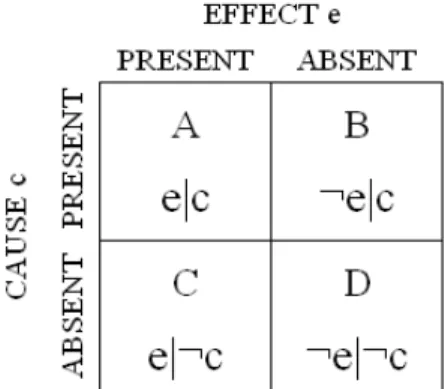
While of course both causes and effects may take the form of stimuli whose properties are on a continuum (such as the brightness of a light or the loudness of a tone), most models of causal learning simplify the problem by defining cause and effect as either present or absent. Researchers generally agree that the statistical information we receive with regard to the presence or absence of candidate causes and effects is computed in some way to assess the covariation between them, which can then form the basis for a causal judgment. At the root of most covariation models is the 2×2 contingency matrix, as shown in Figure 1.1, which describes in the most simple format the possible combinations in which cause and effect can be either present or absent. Exactly how this information is computed is still the subject of rigorous debate (Buehner, Cheng, & Clifford, 2003; Cheng, 1997; Cheng & Novick, 2005; Lober & Shanks, 2000; Luhmann & Ahn, 2005; White, 2005) and numerous models with varying degrees of complexity have been proposed to account for this computation.
One of the best known and widely used models is the ∆P statistic (Jenkins & Ward,
1965). In fact such is the popularity of this measure that it is often treated as an objective
measure of contingency and “contingency” is sometimes used as a synonym for ∆P. The
value of ∆P is given by the difference between the probability of the effect in the presence
of the cause, P(e|c), and the probability of the effect in the absence of the cause, P(e|¬c). In
terms of the cells of the contingency matrix, this is calculated as: ∆P = P(e|c) – P(e|¬c) = A/(A+B) – C(C+D)
There are of course different ways in which the cells of the table may be combined,
including among others the ∆D rule, calculated as (A+B) – (C+D). For an overview of a
number of such rules, see Hammond and Paynter (1983). More recently developed models, for instance Cheng’s (1997) Power PC theory, have extended covariation-based models to
account for some of the particular phenomena of causal inference that ∆P alone cannot
represent. While the discourse continues over how covariation information is and should be utilized in making causal inferences, all researchers would likely agree with the general principle that the greater the contingency between cause and effect, the stronger the perception of causality.
Figure 1.1: Standard 2×2 contingency matrix, showing the four possible combinations of cause and effect occurrence and non-occurrence.
1.4.3 Contiguity
The second of Hume’s tenets, contiguity, refers to the proximity of the cause and effect both in space and in time – spatial and temporal contiguity. In a classic illustration of the importance of contiguity, Michotte (1946/1963) used simple visual stimuli to demonstrate the “launching” effect. A prototypical procedure began with two squares (X and Y) separated from each other by a small distance. X then began to move in a straight line towards Y. On reaching Y (so that their outer surfaces appear to make contact), X stopped moving and Y immediately began to move along the same trajectory. Such a sequence created the strong impression that X collided with Y and caused Y to move. Reports from Michotte’s participants revealed that if Y began to move only after a delay (lack of temporal contiguity), or before it was reached by X (lack of spatial contiguity), the causal impression of X having launched Y was destroyed.
However, as alluded to earlier, a distinction may be drawn between causal perception, which involves a direct interaction and visible physical contact between the
participants in the causal relation, and causal induction, when the physical interaction
between participants is undetectable and the relation must instead be inferred (Cavazza, Lugrin, & Buehner, 2007; Schlottmann & Shanks, 1992; Scholl & Nakayama, 2002). While spatial contiguity remains of utmost importance for perceptual causality (as in the above example of launching), in the case of causal induction (such as in the earlier example of inferring the causes of disease), the necessity of spatial contiguity tends to be downplayed. After all, many events can often be triggered remotely, such as flipping a switch at one end
of a room to cause a light to come on at the other end. Most contemporary research on causal inference instead then focuses on temporal rather than spatial contiguity.
Relatively speaking, there has been far less empirical attention devoted to contiguity compared to contingency (although the disparity is gradually being redressed in recent years). As a result, contiguity is less well understood and its role in causal learning more uncertain. According to Hume, contiguity between cause and effect is essential to the process of causal induction. This supposition was affirmed in a systematic investigation by Shanks, Pearson and Dickinson (1989). Their task involved judging how effective pressing the space-bar on a keyboard was in causing a triangle to flash on a computer screen. Participants were given a fixed amount of time to engage on the task and could gather evidence through repeatedly pressing the space-bar and observing whether or not the outcome occurred. The apparatus was set up to deliver the outcome with a 0.75 probability when the space-bar was pressed. On each trial, if an outcome was scheduled, it would occur after a specific amount of time following the space-bar. This interval varied between conditions from 0 up to 16s. It was found that as the delay increased, participants’ causal judgments decreased in systematic fashion. In fact, conditions involving delays of more than 2s were no longer distinguished as causally effective and were judged just as ineffective as non-contingent control conditions.
Shanks et al.’s (1989) results provided evidence that delays have a deleterious effect on impressions of causality, corroborating the assertions of Hume that contiguity is indeed necessary for causal learning. Yet this idea seems at odds with everyday cognition. Humans and other animals often demonstrate the ability to correctly link causes and effects that are separated in time and learn causal relations involving delays of considerable length; over days, weeks, even months at a time – an often cited example is the temporal gap between intercourse and birth (Einhorn & Hogarth, 1986). And yet, Shanks et al. show a failure to detect causal relations involving gaps of more than a few seconds. C learly there must be something that enables us to bridge such temporal gaps and infer delayed causal relations.
Einhorn & Hogarth (1986) proposed a knowledge mediation hypothesis. They argue that rather than being essential, the function of contiguity is as a cue to direct attention to the contingencies between events. According to this view, people can overcome the requirement for events to be contiguous if there is some other reason why an attentional
link should form between these events; for example, if they have knowledge of some existing mechanism that may connect one to the other. Some knowledge of human biology might therefore enable the connection between intercourse and birth. According to this view, if there is an expectation for a delayed mechanism, a temporal delay no longer becomes an obstacle to causal inference. Thus prior knowledge can mediate the impact of temporal delays.
Adopting this perspective, Buehner and May (2002) demonstrated the detrimental effect of delay could be mitigated by invoking high- level knowledge in participants. In judgment tasks where a cover story was used to make a delay between cause and effect seem plausible (the effect was an explosion and the candidate cause was the launching of a grenade), causal ratings were significantly less adversely affected by delays compared to situations where the cover story made delay seem implausible (where the effect was a lightbulb illuminating and the candidate cause was pressing a switch). Further work by Buehner and May (2004) showed that the effect of delay could be abolished completely by providing explicit information regarding the expected timeframe of the causal relation. Participants again evaluated the effectiveness of pressing a switch on the illumination of a lightbulb; however one group of participants were told that the bulb was an ordinary bulb that should light up right away, while another group of participants was instructed that the bulb was an energy-saving bulb that lights up after a delay. For this latter group there was no decline in ratings with delay; delayed and immediate causal relations were judged as equally effective. Indeed in some circumstances, delays even may serve to facilitate causal attribution where an immediate consequence is incompatible with an expected mechanism (Buehner & McGregor, 2006).
Additionally, Buehner and May (2003) also found that mediation of delay could also be induced through prior experience; they found strong order effects such that where conditions with immediate causal relations preceded conditions with delayed relations, causal ratings were markedly lower compared to when delayed causal relation conditions were presented first. Reed (1992) and Young, Rogers and Beckmann (2005) show that filling an interval with a stimulus such as an auditory tone (known as “signalling”) can likewise negate the impact of delays. Greville, Cassar, Johansen, and Buehner (2010) have meanwhile shown that delays of reinforcement no longer impair instrumental learning
when the task environment highlights the underlying contingency structure. Such work provides insight as to how causal inference can take place over longer time periods. Nevertheless, most researchers agree that in the absence of such mitigating information as described above, delays tend to have a deleterious effect on causal learning, and temporal contiguity thus remains an important cue to causality. Barring a few exceptions, all other things being equal, contiguous causes and effects elicit a stronger causal impression than causes and effects separated by a delay.
1.5 Theories of Causal Learning
Despite a fairly general consensus over the importance of Hume’s cues to causality, there is considerable disagreement with regard to the processes that underlie causal inference. Moreover, no model of learning thus developed has thus provided a full account of causal learning that encompasses its various idiosyncrasies. Dissatisfaction with existing accounts has led to the development of a veritable smorgasbord of learning rules and models over the years, some with the intention of addressing specific facets of learning that previous efforts could not account for, and some providing a more general framework. Each is motivated from a particular theoretical stance, and each has had its successes and shortcomings debated, some more favourably so than others. One long-standing measure,
∆P, has already been briefly described. Others include the probabilistic contrast model
(Cheng & Novick, 1990); Power PC (Cheng, 1997); the pCI rule (White, 2003); BUCKLE (Luhmann & Ahn, 2007); knowledge-based causal induction (Waldmann, 1996); causal support (Griffiths & Tenenbaum, 2005); and theory-based causal induction (Griffiths & Tenenbaum, 2009). While these examples specifically address human causal learning, models of animal conditioning have also been applied (with varying degrees of success) to account for causal inference, including the Rescorla-Wagner model (1972); the SOP model (Wagner, 1981); the Pearce-Hall (1980) and Pearce (1987) models; scalar expectancy theory (Gibbon, 1977); and rate estimation theory (Gallistel & Gibbon, 2000b). Neither of these lists are exhaustive and it is of course unfeasible to accommodate a detailed explanation of all existing models of causal learning within this thesis. Indeed, a full account of a single more complex framework such as theory-based causal induction could easily stand alone as a doctoral thesis in itself (see, e.g., Griffiths, 2005). Instead it seems
more appropriate to categorise these models based on their common ground, and consider the general principles underlying each particular theoretical position. It is also worthwhile to point out at this juncture that the work contained in this thesis examines only generative causes. Accordingly the following review of existing models of causal learning will focus on the generative form.
1.5.1 Conditioning and Associative Learning Theory
Learning in animals is measured by changes in behaviour. Indeed, it has been argued that learning is, by definition, a change in behaviour and that such changes are the only way by which learning can be measured (Baum, 1994). Stimuli that elicit a change in the behaviour of an organism may be categorized as either reinforcers, which increase the frequency of a behaviour, or punishments, which decrease the frequency of a behaviour. The common conception of reinforcement or punishment is the delivery of a stimulus that has a particular motivational significance or adaptive value to the organism; either an appetitive (pleasant) stimulus, such as food, or an aversive (unpleasant) stimulus, such as shock, which are known as primary reinforcers (or punishments). Appetitive stimuli are also often referred to as rewards, and the terms reward and reinforcer are sometimes used interchangeably. However strictly speaking this is not entirely accurate. While appetitive stimuli (rewards) generally serve as reinforcers and aversive stimuli as punishments, this is not always the case; for instance in the case of a satiated animal, food will often fail to increase the frequency of a behaviour and thus cannot be classed as a reinforcer. To clarify then, reinforcement and punishment refer to the effects on behaviour, whereas appetitive and aversive refer to the nature of the stimuli. Reinforcements and punishments are directly responsible for the emergence and maintenance of new behaviour.
The experimental analysis of animal learning and behaviour began with the pioneering work of Ivan Pavlov (1849-1936) and Edward Thorndike (1874-1949) who respectively developed the protocols of classical (Pavlovian) and instrumental conditioning (see Pavlov, 1927; Thorndike, 1898). In a typical classical conditioning preparation, subjects are presented with a neutral stimulus to which they normally would not respond such as a tone or light, referred to as the conditioned stimulus (CS), which is then routinely paired with another stimulus that has some adaptive value (i.e. a primary reinforcer, such as food) and that normally would elicit a response (such as salivation), referred to as the
unconditioned stimulus (US). As conditioning progresses, a new pattern of behaviour is seen to emerge such that the animal responds to the CS before the US is presented or even if the CS is presented in isolation. This is known as the conditioned response (CR) and tends to be similar in nature (though not always identical) to the unconditioned response (UR) that would normally be elicited by the US. Pavlov’s dogs, for instance, after repeatedly hearing a bell ring prior to being fed, developed a salivatory response to the sound of the bell. The presentation of the CS and subsequent delivery of the US in classical conditioning are arranged by the experimenter and thus not dependent on the animal’s behaviour. In an instrumental conditioning protocol meanwhile, a response is required from the animal before the satisfying outcome is obtained. In a typical experiment, Thorndike placed a cat inside a puzzle box, from which it could escape by triggering the appropriate mechanism. Thorndike noted that the time taken for the cat to escape decreased over successive trials, and thus concluded that the animal learned to perform the correct response to evoke the desired consequence of escape. The consequence thus reinforces the response.
Conditioning is thus an example of associative learning. The animal associates the
CS with the US in classical conditioning, and the response with the reinforcer in instrumental conditioning. Through associative learning, stimuli that would not themselves directly evoke an unconditioned response may acquire a motivational function and thus serve as secondary reinforcers. Virtually any stimulus has the potential to provide secondary reinforcement, with money an obvious example in human society. Money in fact serves as a generalized secondary reinforcer through association with many primary reinforcers (since it can be exchanged for food, water, shelter, and even sex) which is why it can exert such powerful effects on behaviour. Associative learning is one of the most fundamental forms of learning and is ubiquitous in the behaviour of organisms, from humans to slime mould (Latty & Beekman, 2009). The parallels between associative learning and causal learning should be immediately apparent, and causal learning is indeed susceptible to many of the same influences as associative learning (Shanks & Dickinson, 1987), as shall now be further discussed.
1.5.1.1 The Rescorla-Wagner Model
Probably the most influential model of learning ever developed is the associative model of Rescorla and Wagner (1972) which at time of writing has been cited in over 3500
scholarly articles. The Rescorla-Wagner model (RWM) has enjoyed such tremendous success due to its simplicity, elegance, and moreover due to its ability to account for various phenomena of conditioning such as blocking (Kamin, 1969). The model was developed specifically as an account of Pavlovian conditioning, and specifies the change in associative strength between CS and US on a given conditioning trial according to the following equation:
∆V = αβ(λ – ΣV)
where ∆V is the change in associative strength, α is the salience of the CS, β is the learning
rate parameter for the US, λ is the current magnitude of the US, and ΣV is the current level
of association between the CS and US (summed over previous trials) for each CS present
on the current trial. More simply, we may term λ as the actual outcome and ΣV the
expected outcome. The RWM is thus a trial-based error-correction model where the animal learns through surprise, in other words through the discrepancy between what is expected to happen and what actually happens.
A trial on which the US follows the CS serves to increase associative strength between them, with successive CS-US pairing resulting in (increasingly smaller) increments in associative strength until the maximum level of association is reached, and
learning has reached asymptote. If the US is absent on a given trial, then λ is 0 and there
will be no increment in associative strength. Indeed if some conditioning has already taken
place, ΣV will be positive and ∆V will hence be negative, producing a decrement in
associative strength. Nonreinforcement thus weakens an existing association. Associative learning then, as specified by the RWM, is sensitive to the statistical relation or contingency between CS and US just as the contingency between cause and effect shapes causal inference.
One of the most notable successes of the RWM was its ability to account for cue competition. This phenomenon was first observed by Kamin (1969) who demonstrated a “blocking” effect in aversive conditioning with rats. In what is now the standard blocking
paradigm, the subject initially received CS1 US in an initial training phase before
undergoing subsequent training with a compound stimulus CS1CS2 US (in Kamin’s
experiments, the US was a shock, CS1 a light, and CS2 a tone). At test, subjects exhibited a
with CS1 alone. Learning the CS1 US association thus appeared to block learning about
CS2, providing clear evidence of competition for associative strength between cues.
Blocking is easily explained by the RWM. Since by the end of phase 1, the US is perfectly
predicted by CS1, there is no discrepancy between the expectation and outcome. In phase 2
then where CS2 is presented, λ is equal to ΣV and hence ∆V is 0. CS2 thus fails to acquire
associative strength. Despite a clear predictive relationship between CS2 and the US in the
second training phase, CS2 is redundant as a predictor because CS1 has already been
established as a perfect predictor of the US. The blocking effect thus further emphasized the sensitivity of conditioning to the statistical relationship between events.
1.5.1.2 The Role of Time from an Associative Perspective
In addition to the statistical relations between cues and outcomes, conditioning is also highly sensitive to the temporal arrangement of events. Indeed, prior to the development of models such as the RWM, contiguity was held to be the dominant principle of learning in traditional associative theories (Gormezano & Kehoe, 1981), with the “Law of Contiguity” stating that if two events occur simultaneously, then the reoccurrence of one event will automatically evoke a memory of the other. In other words, contiguity was considered to be both necessary and sufficient for the formation of an association. Though this assertion has since been toned down in light of new evidence (as shall be discussed further on), contiguity remains a central determinant for conditioning.
The importance of contiguity has been made evident through the comparison of
different conditioning protocols. In what is known as delay conditioning, the CS will first
be presented and the US then delivered either while the CS is still present (so CS and US overlap) or else immediately following CS termination. The delay between CS and US onset is referred to as the interstimulus interval (ISI). Meanwhile, there is an interval
separating CS termination and US onset, this is known as trace conditioning, as
conditioning is assumed to rely on a trace memory or representation of the CS, since it is no longer present. The terminology can sometimes be confusing – in trace conditioning there is a delay separating CS and US, while in delay conditioning the US paradoxically follows the CS without delay. The “delay” in the term instead refers to that between CS and US onset, and serves to distinguish from simultaneous conditioning where CS and US onset is concurrent. It is well-established that (generally) trace conditioning is less effective than
delay conditioning, and that long-delay conditioning less effective than short-delay conditioning, with the CR taking longer to develop (Solomon & Groccia-Ellison, 1996; Wolfe, 1921) and being diminished either in magnitude (Smith, 1968) or in rate (Sizemore & Lattal, 1978; Williams, 1976). Indeed with longer trace intervals, conditioning can fail to occur altogether (Gormezano, 1972; Logue, 1979), though this is highly dependent on the nature of the stimuli entering in the relationship, as the following paragraph shall explain. The influences of temporal contiguity can be incorporated into models of conditioning such
as the RWM by adjusting the value of parameters such as αand β.
Yet, just as with causal learning, there are exceptions to this contiguity principle. The blocking effect, in addition to showing the sensitivity of conditioning to the statistical relationship between events, demonstrated that contiguity alone was not sufficient for conditioning to occur. Although a cue and an outcome may occur contiguously, an association between the two will not be learned if the cue is redundant as a predictor. Furthermore, there is evidence to suggest that a lack of contiguity is not necessarily a barrier to associative learning. In studies by John Garcia and colleagues involving conditioned taste aversion (now commonly dubbed the Garcia effect), rats were given a gustatory stimulus (such as flavoured water) followed by the inducement of nausea (through administration of x-rays, or substances such as lithium chloride or apomorphine hydrochloride), and subsequently demonstrated avoidance reactions to the gustatory stimulus. Importantly, this conditioned taste aversion was readily established even when the onset of nausea is delayed by more than an hour after the gustatory stimulus (Garcia, Ervin, & Koelling, 1966). In an extension of this work, Schafe, Sollars and Bernstein (1995) have shown that rats fail to acquire conditioned taste aversions when the CS-US interval is very brief. Such results indicate that not only is contiguity not always essential for conditioning, but it can actually prevent conditioning in certain circumstances. These findings have been explained by postulating an innate bias such that certain cues and consequences are more readily associable, with these hard-wired preferences presumed to have arisen through natural selection. Garcia and Koelling (1966) indeed demonstrated that particular outcomes tend to become associated with particular stimuli, even when other stimuli are presented concurrently and thus have equal predictive value. While rats in their experiments associated internal malaise with gustatory stimuli, they associated external pain (e.g.
electric shock) with contextual cues such as tones or lights rather than a substance they consumed (demonstrated in their subsequent behaviour).
Broadly speaking then, the core factors of contingency and contiguity appear to exert remarkably similar influences on both the acquisition of associations in classical and instrumental conditioning and on human judgment of causal efficacy. These parallels have led to speculation that causal inference and conditioning are governed by the same underlying processes, and many researchers have attempted to reduce causal inference to associative learning (Allan, 1993; Alloy & Tabachnik, 1984; Dickinson, 2001; Dickinson, Shanks, & Evenden, 1984; Le Pelley & McLaren, 2003; Shanks & Dickinson, 1987; Van Hamme & Wasserman, 1993). In an associative account of causal learning, the cause is mapped to the cue (CS) and the effect to the outcome (US). The strength of a causal impression is then a direct reflection of the acquired associative strength between cues and outcomes, which is continually updated over successive learning opportunities or trials. The demonstration of blocking in human contingency judgment gave further credence to this idea (Shanks, 1985), although a modified RWM (Van Hamme & Wasserman, 1994) is required to encompass backwards blocking (in which phase 1 and phase 2 are switched so subjects are first trained with the compound stimulus).
1.5.1.3 Difficulties for an Associative Account of Causality Judgment
Associative learning theory recognises that the extent of delay that can be tolerated for an association to be learned between stimuli depends on the nature (e.g. the physical attributes) of those stimuli (Shanks, 1993). However, while a bias in the associability of stimuli is plausible with regard to a few evolutionarily significant relations, such as that between taste and nausea, one may often encounter delayed mechanisms that do not have any such connection to physiological processes. In human society in particular, day-to-day life leads us to interact with many artificially developed mechanisms that are not found in the natural environment and thus for which innate knowledge could not possibly have been fostered through natural selection. How then can temporal gaps be bridged in these cases? Associative accounts of causality judgment suggest that stimuli may have differential associative weights that have been transferred from previous learning sessions, which indeed may account for order effects pertaining to contiguity (Buehner & May, 2003). However associationism cannot account for different interpretations of identical evidence
achieved through abstract concepts, such as implicit manipulation of timeframe assumption (Buehner & May, 2002). Thus, it is appropriate to consider other theories which acknowledge other means whereby the connection between a candidate cause and a temporally distant effect may be bridged.
1.5.2 Causal Mechanism and Power Theories
A significant aspect of traditional associative theories is that they inherited Hume’s empiricism; they are data-driven or “bottom-up” in the sense that only the observable properties of stimuli such as contiguity are considered to contribute to learning. However, a number of findings have proven problematic for this empiricist approach applied to causal inference. People appear to have pre-existing conceptions both about the types of stimuli that are able to elicit certain outcomes and the timeframes involved in such processes, and can use this knowledge to guide causal inference (Buehner & May, 2002, 2004; Einhorn & Hogarth, 1986). Purely bottom- up accounts do not allow the scope for influences such as higher- level knowledge on learning and therefore struggle to explain such effects where there is no plausible prior associability bias. Alternatives to the empiricist approach therefore embrace instead the philosophical position of Immanuel Kant (1781/1965), who proposed that people have intuitive ideas about causality that provide a framework for learning new relations. That is, causal relations need not be derived solely from empirical observation; inference may also be facilitated or constrained by top-down information.
Causal mechanism or power theories of causal learning stem from the Kantian rather than the Humean perspective. The central underlying principle of this view is that successful causal inference hinges upon belief in or knowledge of a causal mechanism – a specific process connecting causes to their effects and thus creating an intuition of necessity between the two (Ahn, Kalish, Medin, & Gelman, 1995; White, 1989). According to this view, causes are not just passively followed by effects, but rather actively generate their effects by exerting their causal power. This may be seen as the transmission of force, energy or some other property from one element to another (Peter A. White, 2009). This position is motivated by the same cautionary mantra that is drummed into any aspiring scientist or statistician; that correlation or covariation does not necessarily imply causation. The key contribution then of mechanistic knowledge is in making the mental leap from an observed covariation to the inference of a causal relation. It is therefore considered that
people do not infer causality unless they know of a plausible mechanism by which these events could be linked. Such a perspective has however been criticised as being hamstrung by circularity: If top-down assumptions about mechanism govern causal inference, where do such assumptions come from in the first place?
1.5.2.1 The Power PC Theory
Cheng (1997) attempted to synthesize the ideas of Hume and Kant, and refine the causal power account, by proposing that empirically observable data (in the form of contingency information) serves as the initial input for causal learning, while prior knowledge then guides inferences drawn from this data. The prior causal knowledge assumed here is general rather than specific. That is, mechanistic knowledge that is initially acquired from empirical observations can then subsequently then be generalized to novel learning situations (see Liljeholm & Cheng, 2007), hence overcoming the problem of circularity.
According to Cheng (1997), observed deviations in human causal judgments from
measures such as ∆P are due to fundamental assumptions that people make about the nature
of causality that go beyond mere covariation, such the assumption of causal power. Such
deviations in judgement include sensitivity to changes in the base rate of the effect, P(e|¬c),
when ∆P is constant. To address these shortcomings of ∆P, Cheng advanced the power
theory of the probabilistic contrast model, usually shortened to PowerPC. This approach focuses on the generative (or inhibitory) power of the cause, that is, its capacity to produce (or prevent) the effect independently of all other potential causes. Causal power is computed as:
∆P / 1 – P(e|¬c) for generative causes
–∆P / P(e|¬c) for preventative causes
Causal power is thus further distinguished from covariation models by making different predictions from identical contingency data depending on whether the cause is assumed to be generative or preventive, providing greater flexibility. One well-documented phenomena of causal induction that covariation models cannot account for but that is predicted by Power PC is the problem of ceiling effects. For example suppose one wished to test whether a new type of medication produced nausea as a side effect. If every participant
that the medication was a very strong cause of nausea. But suppose every participant was feeling nauseous to begin with; the results would then be uninterpretable; the participant might well have developed nausea after taking the medication but since they were already
feeling nauseous this cannot be evaluated. ∆P in this case would be zero; P(e|c) – P(e|¬c) =
1 – 1 = 0, therefore predicting that the medication would be judged as noncausal. In contrast the Power PC model, taking the generative form of the equation, would not return a value in such a case, as the equation attempts to divide by zero. Power PC thus correctly predicts that humans in such a situation would refrain from making a causal judgment rather than concluding that the medication does not cause nausea.
In similar fashion, consider again the above clinical trials scenario but instead assume that the medication was supposed to prevent (or relieve) nausea. Since none of the participants experienced relief, one can, in this case, rationally conclude that the medication
was ineffective as a preventive cause of nausea. The predictions of causal power and ∆P
here then are equivalent for the preventive case but differ in the generative case when P(e|c)
= P(e|¬c) = 1. Meanwhile, if the base rate was zero and once again P(e|c) = P(e|¬c), causal
power predicts that humans will be unable to make a causal inference in the preventive case
(as there is no opportunity for the cause to exert its effect) but will accord with ∆P in the
generative case.
Predictions of the PowerPC model thus more closely mirror human judgments than
∆P and have proven resilient to challenges from other researchers (see Buehner et al.,
2003). However, although PowerPC emphasizes the distinction between causation and
covariation, causal power is still computed using covariation information – indeed, the ∆P
statistic itself forms part of the Power PC model. The causal power perspective therefore makes the assumption that an observed configuration of causes and effects can be unambiguously interpreted to populate the cells of the contingency table. However, this is not necessarily a given. Furthermore, the model does not explicitly represent temporal information.
1.5.2.2 The Role of Time from Covariation Perspectives
From the causal power view and related perspectives, time is not bestowed with a particularly privileged role in causal learning. Temporal information is instead used to determine how events experienced in the input are assigned to the cells of the 2×2
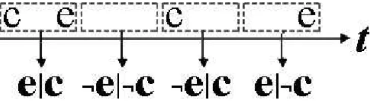
contingency matrix. Provided that this information can be discerned from the available evidence, contiguity is not required to compute contingency. If there is temporal separation between cause and effect, the assumptions regarding mechanism and the expectation of timeframe determines how these events are interpreted. If a delay is anticipated, then the
effect will be attributed to the cause, and constituting a single case of cell A (ce, or e|c),
as shown in Figure 1.2, strengthening the causal impression. If instead a contiguous
mechanism is expected, a delayed pairing will be interpreted as one case of cell B (c¬e
or ¬e|c) and one case of cell C (¬ce or e|¬c), weakening the causal impression. This is
known as the attribution shift hypothesis (Buehner, 2005). Contiguity is thus only a
necessity if a contiguous mechanism is expected; meanwhile longer delays can be tolerated if a slower mechanism is hypothesized. Longer intervals however also increase the likelihood of intervening events occurring between action and outcome, which compete for explanatory strength and place greater demands on processing and memory resources. Delays thus introduce added uncertainty as to whether a given effect was generated by the cause in question or whether it was produced by some other mechanism. This can mean that causal learning with delays may sometimes be problematic even when the anticipated mechanism means delays are plausible.
Figure 1.2: The effect of attribution shift in parsing an event stream with a specific
timeframe assumed : c e intervals that are longer than the temporal window
simultaneously decrease impressions of P(e|c) and P(¬e|¬c) while increasing impressions
of P(e|¬c) and P(¬e|c).
The causal power and mechanism theories thus reflect the view that learners adopt a more active approach to inferring causality. Rather than just passively processing information, we seek to impose structure on data, using heuristics and prior knowledge to constrain causal inference. Such mechanistic beliefs are key to avoiding learning spurious
relations. We do not, for example, learn that the crowing of a rooster causes the sun to rise, despite the fact that former event reliably signals the latter, since we know of no plausible mechanism by which the rooster crowing could influence the rising of the sun. A key strength of such approaches to causal learning is thus the flexibility to allow for top-down influences such as prior knowledge to assist in the comprehension of empirical sensory data. From this perspective then, causal learning is more than the mere sum of its parts. 1.5.3 Causal Models and Structure Theories
A third perspective on causal learning embraces a framework developed in statistics and computer science – probabilistic graphical models (Glymour, 2001; Pearl, 2000; Spirtes, Glymour, & Schienes, 1993). As the name suggests, this framework utilizes graphs to model probabilistic relations in a simple yet effective manner, in which variables such as causes and effects are denoted by nodes, and causal connections are indicated by arrows linking these nodes. These models are also commonly referred to as causal Bayesian networks (often shortened to Bayes nets), since their application utilises principles of Bayesian probabilistic inference. Named after its original proponent Reverend Thomas Bayes (1702–1761), Bayesian inference is a form of logical reasoning whereby the probability of a hypothesis is assessed by specifying some prior probability which is then updated in the light of new, relevant data.
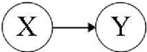
Figure 1.3 shows a graphical model expressing the causal relation “X causes Y”. This is a prototypical example of a directed acyclic graph (DAG); directed in the sense that X and Y are connected by a directed arrow from X to Y, rather than by an undirected link; and acyclic as there is no corresponding arrow directed from Y to X, and so a path cannot be traced from one node back to itself. DAGs are the most popular means of expressing causal relations in a graphical model, and the intuitive simplicity of these models makes them a effective tool for representing complex causal networks.
The fact that the causal arrow extends from X to Y with no symmetrical link from Y to X reflects causal directionality, such that X causes Y but Y does not cause X. A crucial component to causal understanding is that causes produce their effects and not vice versa, such that an alteration to X will consequently produce an alteration in Y, but that an alteration to made directly to Y itself will not produce an alteration in X. The representation of directionality is one of a number of key advantages afforded by Bayes nets.
1.5.3.1 Causal Model Theory
Waldmann and Holyoak (1992, 1997) argued that principles such as directionality cannot be captured by mere associations, and pinpointed this failure to specify causal direction as a major shortcoming of associative theories of causal learning. Waldmann and
Holyoak instead advocated a causal model theory, according to which humans have a
strong tendency to learn directed links from causes to effects, rather than vice versa, in line with how information is represented in a causal graphical model. Importantly, this remains the case even when an effect is observed temporally prior to the cause – for example, when one sees smoke before one sees the fire that produces it. In such a case, the smoke is still correctly identified as an effect of a temporally precedent cause, the fire, even if the fire is seen only subsequently, or remains unseen. In other words, humans construct causal models that correspond to the veridical temporal order rather than the perceived temporal order.
Inferring the presence of fire from the observation of smoke is an example of diagnostic inference. Waldmann and Holyoak (1992) drew special attention to the idea that people appear able to reason both predictively, from causes to effects, or diagnostically, from effects to causes. In a typical conditioning preparation, the order of stimulus presentation mirrors the temporal order of a predictive causal model. Cues (input) correspond to causes, and effects to outcomes (output). According to an associative account of causal learning, the strength of a perceived causal relation is assumed to be a reflection of the associative strength between cues and outcomes (Van Hamme, Kao, & Wasserman, 1993). However as Waldmann and Holyoak illustrate, in diagnostic inference the input-output sequence is reversed with respect to the true causal model. In an associative account of causal learning, effects would be assigned to the input layer and causes would be assigned to the output layer, based on the order of observation in a diagnostic causal model.