Semi-Markov Models for Named Entity Recognition
Sunita Sarawagi Indian Institute of Technology
Bombay, India [email protected]
William W. Cohen
Center for Automated Learning & Discovery Carnegie Mellon University
[email protected] Zhenzhen Kou
Center for Automated Learning & Discovery Carnegie Mellon University
Abstract
We described semi-Markov models which relaxes usual Markov assumptions made in hidden Markov mod-els. Semi-Markov models classifysegmentsof adjacent words, rather than single words. We proposed two training strategies, a discriminative training and a generative training for semi-Markov models. Importantly, features for semi-Markov models can measure properties of segments, and transitions within a segment can be non-Markovian. This formalism can incorporate information about the similarity of extracted entities to entities in an external dictionary. This is difficult because most high-performance named entity recognition systems operate by sequentially classifying words as to whether or not they participate in an entity name; however, the most useful similarity measures score entire candidate names. In addition to allowing a natural way of coupling high-performance NER methods and high-performance similarity functions, this formalism also allows the direct use of other useful entity-level features, and provides a more natural formulation of the NER problem than sequential word classification. We applied semi-Markov models to named entity recog-nition (NER) problems and in experiments on eight datasets, semi-Markov models generally achieved better performance, especially when there is not much available training data, semi-Markov models can achieve significantly better accuracy than other baseline algorithms via incorporating information from an external dictionary.
Keywords:Learning, sequential learning, semi-Markov models, information extraction, named entity recognition.
1 Introduction
Collective classificationhas been widely used for classification on structured data. In collective classification, classes are predicted simultaneously for a group of related instances, rather than predicting a class for each instance separately. Recently there have been studies on relational models for collective inference, such as relational dependency networks [23], relational Markov networks [49, 8], and Markov logic networks[39]. Collective classification can be formulated as an inference problem over graphical models. Consider collective classification in the context of Markov random fields (MRFs). Although collective inference has been shown to be able to achieve good performance, inference in MRFs is intractable except for special cases, notably trees or linear-chains. Linear-chains are widely used in natural language processing. Therefore in this paper we aim to extend representational power of a Markov chain without losing polynomial-time exact inference.
In this paper We studied semi-Markov models (SMMs), which relax the usual Markov assumptions made in linear-chain systems. Recall thatsemi-Markov chain modelsextend hidden Markov models (HMMs) by allowing each statesito persist for a non-unit length of timedi. After this time has elapsed, the system will transition to a new states0, which depends only onsi;
however, during the “segment” of time betweeniandi+di, the behavior of the system may be non-Markovian. Generative semi-Markov models are fairly common in certain applications of statistics [18, 22], and are also used in reinforcement learning to model hierarchical Markov decision processes [46].
SMMs has polynomial-time exact inference. If relaxing the assumptions in linear Markov chains further and adding more dependencies among the non-adjacent nodes, the linear-chain system will be turned into MRFs and the inference will be intractable. The long-term goal of our study is to combine more powerful exact inference methods with approximate inference. Named entity recognition (NER) is finding the names of entities in unstructured text. We investigated the task of improving NER systems using semi-Markov models in our paper.
Below we will present semi-Markov models and describe two learning algorithms– a generative model and a discriminative model, in Section 2 and Section 3. We then present experimental results in Section 4 and Section 5, and conclude in Section 6.
2 Semi-Markov Models for Named Entity Recognition
2.1 Named Entity Recognition as Word Tagging
Named entity recognition is the process of annotating sections of a document that correspond to “entities” such as people, places, times and amounts. As an example, the output of NER on the email document
Fred, please stop by my office this afternoon. might be
(Fred)Personplease stop by (my office)Location(this afternoon)Time
A common approach to NER is to convert name-finding to ataggingtask. A document is encoded as a sequencexof tokens x1, . . . , xN, and ataggerassociates withxa parallel sequence of tagsy=y1, . . . , yN, where eachyiis in some tag setY. If these tags are appropriately defined, the name segments can be derived from them. For instance, one might associate one tag with each entity type above, and also add a special “other” tag for words not part of any entity name, so that the tagged version of the sentence would be
Fred please stop by my office this afternoon
Person Other Other Other Location Location Time Time
A common way of constructing such a tagging system is to learn a mapping fromxtoyfrom data [3, 5, 33]. Typically this data is in the form of annotated documents, which can be readily converted to(x,y)pairs.
Most methods for learning taggers exploit, in some way, the sequential nature of the classification process. In general, each tag depends on the tags around it: for instance, if person names are usually two tokens long, then ifyi is tagged “Person” the probability thatyi+1is a “Person” is increased, and the probability thatyi+2 is a “Person” is decreased. Hence the most
common learning-based approaches to NER learn a sequential model of the data, generally some variant of a hidden Markov model (HMM) [16].
2.2 Semi-Markovian NER
It will be convenient to describe our framework in the context of one of these HMM variants, in which the conditional distribu-tion ofygivenxis defined as
P(y|x) =
|x| Y
i=1
P(yi|i,x, yi−1)
(Here we assume a distinguished start tagy0which begins every observation.) This is the formalism used in maximum entropy
taggers [38], and it has been variously called a maximum entropy Markov model (MEMM) [34] and a conditional Markov model (CMM) [25]. Inference in this model can be performed with a variant of the Viterbi algorithm used for HMMs. Given training data in the form of pairs(x,y), the “local” conditional distributionP(yi|i,x, yi−1)can be learned from derived triples
We will relax this model by assuming that tagsyido not change at every positioni; instead, tags change only at certain selected positions, and after each tag change, some number of tokens are observed. Following work in semi-Markov decision processes [47, 18] we will call this a semi-Markov model (SMM).
For notation, letS=hS1, . . . , SMibe a “segmentation” ofx. Eachsegmentsj =htj, uj, yjiconsists of astart positiontj, which is an index between 1 andM, anend positionuj, and alabel`j ∈Y. A segmentationSisvalidif∀j,tj =uj−1+ 1.
We will consider only valid segmentations.
Conceptually, a segmentation means that the tag`jis given to allxi’s betweeni =tj andi=uj, inclusive: alternatively, it means that the tagsytj. . . yuj corresponding toxtj. . . xuj are all equal to`j. Formally, letJ(S, i)be the indexjsuch that tj ≤i≤uj, and define thetag sequenceyderived fromSto be`J(S,1), . . . , `J(S,|x|).
For instance, a segmentation for the sample sentence above might be S = {(1,1,Person), (2,4,Oth), (5,6,Loc), (7,8,Time)}, which could be written as
(Fred)Person(please stop by)Other(my office)Location(this afternoon)Time
A CSMM is defined by a distribution over pairs(x,S)of the form P(S|x) = Y
j
P(Sj|tj,x, `j−1) (1)
More generally, we use the termsemi-Markov model(SMM). for any model in which eachSj depends only on the label`j−1
associated withSj−1, and is independent ofSj0 for allj0 6=j,j06=j−1.
Two issues need to be addressed: inference for SMMs, and learning algorithms for SMMs. For learning, inspection of Equa-tion 1 shows that given training in the form of(x,S)pairs, learning the “local” distributionP(Sj|tj,x, `j−1)is not much more
complex than for a CMM.1However, conditionally-structured models like the CMM are not the ideal model for NER systems:
better performance can often be obtained by algorithms that learn a single global model forP(y|x)[12, 29]. Below we will present two learning algorithms: a “global” learning algorithm derived from Collins’ perceptron-based algorithm[12] and a discriminative algorithm derived from CRFs.
For inference, we will present below Viterbi-like algorithms for the generative and discriminative learning algorithms, respec-tively, that find the most probableSgivenxin timeO(N L|Y|), whereNis the length ofxandLis an upper bound on segment length—that is,∀j,L≥uj−tj. SinceL≤N, this inference procedure is always polynomial. (In our experiments, however, it is sufficient to limitLto rather small values.)
We emphasize that an SMM with segment length bounded byL is quite different from an order-L CMM, as in an order-L CMM, the next label depends on the previousLlabels, but not the corresponding tokens. A SMM is also different from a CMM which uses a window of the previousLtokens to predictyi, since the SMM makes asinglelabeling decision for a segment, rather than making series of interacting decisions incrementally. In Section 4.3.3 we will experimentally compare SMM’s and high-order CMMs.
2.3 Probabilistic Training for SMMs: semi-CRFs 2.3.1 Definitions
The generative models for SMMs can be extended from Conditional Random Fields (CRFs). A CRF modelsPr(y|x)using a Markov random field, with nodes corresponding to elements of the structured objecty, and potential functions that are conditional on (features of)x. Learning is performed by setting parameters to maximize the likelihood of a set of(x,y)pairs given as training data. One common use of CRFs is for sequential learning problems like NP chunking [44], POS tagging [29], and NER [35]. For these problems the Markov field is a chain, andyis a linear sequence of labels from a fixed setY.
Assume a vectorf oflocal feature functionsf =hf1, . . . , fKi, each of which maps a pair(x,y)and an indexito a measure-mentfk(i,x,y)∈R. Letf(i,x,y)be the vector of these measurements, and letF(x,y) =P|x|
i f(i,x,y). For example, in NER, the components offmight include the measurementf13(i,x,y) = [[x
iis capitalized]]·[[yi=P erson]],
1The additional complexity is that we must learn to predict not only a tag type`
j, but also the end positionuj of each segment (or
where the indicator function [[c]] = 1 ifc if true and zero otherwise; this implies that F13(x,y) would be the number of
capitalized wordsxipaired with the label “Person”.
Following previous work [29, 44] we will define a conditional random field (CRF) to be an estimator of the form Pr(y|x,W) = 1
Z(x)e
W·F(x,y) (2)
whereWis a weight vector over the components ofF, andZ(x) =Py0eW·F(x,y 0)
.
In Semi-CRFs, sdenotes a segmentation, a vector g denotes segment feature functions andG(x,s) = Pj|s|g(j,x,s). A semi-CRFis then an estimator of the form
Pr(s|x,W) = 1 Z(x)e
W·G(x,s) (3)
where againWis a weight vector forGandZ(x) =Ps0eW·G(x,s 0)
. 2.3.2 A Probabilistic Learning Algorithm
During training the goal is to maximize log-likelihood over a given training setT ={(x`,s`)}N`=1. Following the notation of
Sha and Pereira [44], we express the log-likelihood over the training sequences as L(W) =X ` log Pr(s`|x`,W) = X ` (W·G(x`,s`)−logZW(x`)) (4) We wish to find aWthat maximizesL(W). Equation 4 is convex, and can thus be maximized by gradient ascent, or one of many related methods. (In our implementation we use a limited-memory quasi-Newton method [31, 32].) The gradient of L(W)is the following: ∇L(W) = X ` G(x`,s`)− P s0G(s0,x`)eW·G(x`,s 0) ZW(x`) (5) = X ` G(x`,s`)−EPr(s0|W)G(x`,s0) (6) The first set of terms are easy to compute. However, to compute the the normalizer,ZW(x`), and the expected value of the
features under the current weight vector,EPr(s0|W)G(x`,s0), we must use the Markov property ofGto construct a dynamic programming algorithm, similar for forward-backward. We thus defineα(i, y)as the value ofPs0∈si:yeW·G(s
0,x)
where again
si:ydenotes all segmentations from 1 toiending atiand labeledy. Fori >0, this can be expressed recursively as α(i, y) = L X d=1 X y0∈Y α(i−d, y0)eW·g(y,y0,x,i−d+1,i) (7) with the base cases defined asα(0, y) = 1andα(i, y) = 0fori <0. The value ofZW(x)can then be written asZW(x) = P
yα(|x|, y).
A similar approach can be used to compute the expectation Ps0G(x`,s0)eW·G(x`,s
0)
. For the k-th component ofG, let ηk(i, y)be the value of the sumP
s0∈si:yGk(s0,x`)eW·G(x`,s 0)
, restricted to the part of the segmentation ending at positioni. The following recursion2can then be used to computeηk(i, y):
ηk(i, y) = (8) PL d=1 P y0∈Y(ηk(i−d, y0) +α(i−d, y0)gk(y, y0,x, i−d+ 1, i))eW·g(y,y 0,x,i−d+1,i) (9) Finally we letEPr(s0|W)Gk(s0,x) = Z 1 W(x) P yηk(|x|, y). The training for SemiCRFs are summerized in Figure 1.
2As in the forward-backward algorithm for chain CRFs [44], space requirements here can be reduced fromM L|Y|toM|Y|, whereMis the length of the sequence, by pre-computing an appropriate set ofβvalues.
Probalistic SMM Learning
For each each iteration in the limited-memory auasi-Newton method: 1. Use equation 10 to calculateα(i, y)and getZW(x) =
P
yα(|x|, y). 2. Use equation 12 to calculateηk(i, y)and getE
Pr(s0|W)Gk(s0,x) =Z 1
W(x)
P
yηk(|x|, y).
3. Use euquation 9 to calculate∇L(W)and updateWt+1using the limited-memory quasi-Newton method.
As the final output of learning, returnW, the average of theWt’s. To segmentxwithW, use Equation 12 to find the best segmentation.
Figure 1: Discriminative training for SMM’s. 2.3.3 An Inference Algorithm
The semi-Markov analog of the usual Viterbi algorithm for Semi-CRFs is the same as Equation 12. However, in segmentation models, the primary limitation is the increased computational cost of inference tasks. The inference can be quadratic or even cube in the length of the sequence. A practical solution is to limit the maximum length of a segment by a prior parameterL. 2.4 Features for SMMs
In a semi-Markov learner, features no longer apply to individual words, but instead are applied to hypothesized entity names. This makes it somewhat more natural to define new features, as well as providing more context.
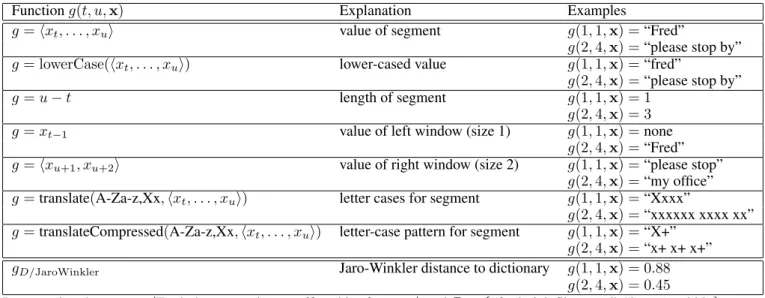
In the notation of this paper, recall that we assumed each SMM feature function fk can be written as fk(j,x,S) = fk(gk(t
j, uj,x), `j, `j−1), wheregk is any function oftj,uj, and the sequencex. Typically, gk will compute some prop-erty of the proposed segmenthxtj. . . xuji(or possibly of the tokens around it), andfk will be an indicator function that couples this property with the label`j. Some concrete examples of possiblegk’s are given in Table 1.
Since any of these features can be applied to one-word segments (i.e., ordinary tokens), they can also be used for a HMM-like, word-tagging NER system. However, some of the features are much more powerful when applied to multi-word segments. For instance, the pattern “X+ X+” (two capitalized words in sequence) is more indicative of a person name than the pattern “X+”. As another example, the “length” feature is often informative for segments.
Since we are no longer classifying tokens, but are instead classifyingsegmentsas to whether or not they correspond to complete entity names, it is straightforward to make use of similarity to words in an external dictionary as a feature. LetDbe a dictionary of entity names anddbe a distance metric for entity names. DefinegD/d(e0)to be the minimum distance betweene0 and any entity nameeinD:
gD/d(e0) = min
e∈Dd(e,e
0)
For instance, ifD contains the two strings “frederick flintstone” and “barney rubble”, andd is the Jaro-Winkler distance metric [50], thengD/d(hFredi) = 0.84, andgD/d(hFred,pleasei) = 0.4, sinced(“Fred”,“frederick flintstone”) = 0.84and d(“Fred please”, “frederick flintstone”) = 0.4. A feature of the formgD/dcan be trivially added to the SMM representation for any pairDandd.
One problem with distance features is that they can be relatively expensive to compute, particularly for a large dictionary. In the experiments below, we pre-processed each dictionary by building an inverted index over the charactern-grams appearing in dictionary entries, forn= 3,4,5, discarding any “frequent”n-grams that appear in more than 80% of the dictionary entries. We then approximategD/d(e0)by finding a minimum over only those dictionary entries that share a common non-frequent n-gram withe0.
We also extended the semi-Markovian algorithm to construct, on the fly, aninternal segment dictionaryof segments labeled as entities in the training data. To make measurements on training data similar to those on test data, when finding the closest neighbor ofxsj in the internal dictionary, we excluded all strings formed fromx, thus excluding matches ofxsj to itself (or subsequences of itself). This feature could be viewed as a sort of nearest-neighbor classifier; in this interpretation the semi-CRF is performing a sort of bi-level stacking [52].
Functiong(t, u,x) Explanation Examples
g=hxt, . . . , xui value of segment g(1,1,x) =“Fred”
g(2,4,x) =“please stop by” g= lowerCase(hxt, . . . , xui) lower-cased value g(1,1,x) =“fred”
g(2,4,x) =“please stop by”
g=u−t length of segment g(1,1,x) = 1
g(2,4,x) = 3
g=xt−1 value of left window (size 1) g(1,1,x) =none
g(2,4,x) =“Fred” g=hxu+1, xu+2i value of right window (size 2) g(1,1,x) =“please stop”
g(2,4,x) =“my office” g=translate(A-Za-z,Xx,hxt, . . . , xui) letter cases for segment g(1,1,x) =“Xxxx”
g(2,4,x) =“xxxxxx xxxx xx” g=translateCompressed(A-Za-z,Xx,hxt, . . . , xui) letter-case pattern for segment g(1,1,x) =“X+”
g(2,4,x) =“x+ x+ x+”
gD/JaroWinkler Jaro-Winkler distance to dictionary g(1,1,x) = 0.88
g(2,4,x) = 0.45 In examples above,x=hFred,please,stop,by,my,office,this,afternooniandD={“frederick flintstone”,“barney rubble}
Table 1: Possible feature functionsg.
of a segment, the values of first and last token in a segment, the letter case and letter case pattern for a segment and its first and last token. Distance featuregD/dis used when there is an external dictionary. Additional dictionary-based binary features are described in Section 4.1.
3 Perceptron-based Training for SMMs
3.1 Perceptron-based TrainingWe also consider a perceptron-based learning algorithm for training SMMs because (a) it is easy to implement, (b) it is justified by large-margin theory, (c) it approximates the CRF optimization method.
The perceptron-based learning algorithm we use for training SMMs is derived from Collins’ perceptron-based algorithm for discriminatively training HMMs, which can be summarized as follows. Assume alocal feature functiongwhich maps a pair (x,y)and an indexito a vector of featuresg(i,x,y). Define
G(x,y) =
|x| X
i
g(i,x,y)
LetW be a weight vector over the components ofG. During inference we need to computeV(W,x), the Viterbi decoding of
xwithW,i.e.,
V(W,x) =argmaxyG(x,y)·W
For completeness, we will outline howV(W,x)is computed. To make Viterbi search tractable, we must restrictg(i,x,y)to make limited use ofy. To simplify discussion here, we assume thatgis strictly Markovian,i.e., that for each componentfkof
g,
fk(i,x,y) =fk(gk(i,x), y i, yi−1)
For fixedyandy0, we denote the vector offk(gk(i,x), y, y0)for allkasg0(i,x, y, y0).
Viterbi inference can now be defined by this recurrence, wherey0is the designated start state:
0 ifi= 0andy=y0 −∞ ifi= 0andy6=y0 maxy0 Vx,W(i−1, y0) +W ·g0(i,x, y, y0) ifi >0
and thenV(W,x) = maxy0Vx,W(|x|, y). Using dynamic programming this can be computed efficiently.
The goal of learning is to find aW that leads to the globally best overall performance. This “best”W is found by repeatedly updatingW to improve the quality of the Viterbi decoding on a particular example(xt,yt). Specifically, Collin’s algorithm starts withW0 =0. After thet-th example(xt,yt), the Viterbi sequenceyˆt=V(Wt,xt)is computed. Ifyˆt=yt,Wt+1is
set toWt, and otherwiseWtis replaced with
Wt+1=Wt+G(xt,yt)−G(xt,yˆt)
After training, one takes as the final learned weight vectorW the average value ofWtover all time stepst.
This simple algorithm has performed well on a number of important sequential learning tasks [12, 2, 44], including NER. It can also be proved to converge under certain plausible assumptions [12].
The natural extension of this algorithm to SMM’s assumes training data in the form of pairs(x,S), whereSis a segmentation. We will assume a feature-vector representation can be computed for any segmentSjof a proposed segmentationS,i.e., we assume a vectorgofsegment feature functionsg=hg1, . . . , gKi, each of which maps a triple(j,x,s)to a measurement gk(j,x,s) ∈ R, and defineG(x,s) = P|s|
j g(j,x,s). We also make a restriction on the features, analogous to the usual Markovian assumption, and assume that every componentgkofgis a function only ofx,s
j, and the labelyj−1associated with
the preceding segmentsj−1. In other words, we assume that everygk(j,x,s)can be rewritten as
gk(j,x,s) =g0k(y
j, yj−1,x, tj, uj) (11)
for an appropriately definedg0k. In the rest of the paper, we will drop theg0 notation and useg for both versions of the
segment-level feature functions.
Then one can apply Collins’ method immediately, as long as it is possible to perform a Viterbi search to find the best segmen-tationSˆfor an inputx. We will now outline the Viterbi search for segments.
LetLbe an upper bound on segment length. Letsi:ydenote the set of all partial segmentations starting from 1 (the first index of the sequence) toi, such that the last segment has the labelyand ending positioni. LetVx,g,W(i, y)denote the largest value of
W·G(x,s0)for anys0 ∈s
i:y. Omitting the subscripts, the following recursive calculation implements a semi-Markov analog of the usual Viterbi algorithm:
V(i, y) =
( maxy
0,d=1...L V(i−d, y0) +W·g(y, y0,x, i−d+ 1, i) ifi >0
0 ifi= 0
−∞ ifi <0 (12)
The best segmentation then corresponds to the path traced bymaxyV(|x|, y). Conceptually,V(i, y)is the score of the best segmentation of the firstitokens inxthat concludes with a segmentSjsuch thatuj =iand`j =y.
3.2 Refinements to the Learning Algorithm
We experimentally evaluated a number of variants of Collins’ method, and obtained somewhat better performance with the following extension. As described above, the algorithm finds the single top-scoring label sequenceyˆ, and updatesW if the score ofyˆis greater than the score of the correct sequencey(where the “score” ofy0 isW ·G(x,y0)). In our extension, we
modified the Viterbi method to find the topKsequencesyˆ1, . . . ,yˆK, and then updateW for allyˆi’s with a score higher than (1−β)times the score ofy.
The complete algorithm is shown in Figure 2. The same technique can also be used to learn HMMs, by replacingSwithyand Equation 12 with Equation 10.
Like Collins’ algorithm, our method works best if it makes several passes over the data. There are thus four parameters for the method:K,β,L, andE, whereEis the number of “epochs” or iterations through the examples.
Perceptron-Based SMM Learning
Letg(j,x,S)be a feature-vector representation of segmentSj, and letG(x,S) =
P|S|
j=1g(j,x,S).
LetSCORE(x, W;S) =W·G(x,S). For each each examplext,St:
1. Use Equation 12 to find theKsegmentationsSˆ1, . . . ,SˆK that have the highestSCORE(xt, Wt; ˆSi). 2. LetWt+1=Wt.
3. For eachisuch thatSCORE(xt, Wt; ˆSi)is greater than(1−β)·SCORE(xt, Wt;St), updateWt+1as follows:
Wt+1←Wt+1+G(xt,St)−G(xt,Sˆi)
As the final output of learning, returnW, the average of theWt’s. To segmentxwithW, use Equation 12 to find the best segmentation.
Figure 2: Discriminative training for SMM’s.
4 Experimental Results
4.1 Baseline Algorithms and Datasets
To evaluate our proposed methods for learning SMMs, we compared the two Semi-Markov models with the HMM-based version of the voted perceptron algorithm and standard CRFs.
As features for thei-th token, we used a history of length one, plus the lower-cased value of the token, letter cases, and letter-case patterns (as illustrated in Figure 1) for all tokens in a window of size three centered at thei-th token. Additional dictionary-based features are described below.
We experimented with two ways of encoding NER as a word-tagging problem. The simplest methods, HMM-VP/1 and CRF/1, predict two labelsy: one label for tokens inside an entity, and one label for tokens outside an entity.
The second encoding scheme we used is due to Borthwicket al[5]. Here four tagsy are associated for each entity type, corresponding to (1) a one-token entity, (2) the first token of a multi-token entity, (3) the last word of a multi-token entity, or (4) any other token of a multi-token entity. There is also a fifth tag indicating tokens that are not part of any entity. For example, locations would be tagged with the five labelsLocunique,Locbegin,Locend,Loccontinue, andOther, and a tagged example like
(Fred)Person, please stop by the (fourth floor meeting room)Loc
is encoded (omitting for brevity the “Other” tags) as
(Fred)Personunique, please stop by the (fourth)Locbegin (floor meeting)Loccontinue(room)Locend
We will call this scheme HMM-VP/4 and CRF/4.
To add dictionary information to HMM-VP/1and CRF/1, we simply add one additional binary featurefD which is true for every token that appears in the dictionary: i.e., for any tokenxi, fD(xi) = 1if xi matches any word of the dictionary D andfD(xi) = 0otherwise. This feature is then treated like any other binary feature, and the training procedure assigns an appropriate weighting to it relative to the other features.
To add dictionary information to HMM-VP/4 and CRF/4, we again follow Borthwicket al[5], who proposed using a set of four features,fD.unique,fD.f irst,fD.last, andfD.continue. These features are analogous to the four entity labels: for each tokenxi the four binary dictionary features denote, respectively: (1) a match with a one-word dictionary entry, (2) a match with the first word of a multi-word entry, (3) a match with the last word of a multi-word entry, or, (4) a match with any other word of an entry. For example, the tokenxi=“flintstone” will have feature valuesfD.unique(xi) = 0,fD.f irst(xi) = 0,fD.continue(xi) = 0, and fD.last(xi) = 1(for the dictionaryDused in Table 1).
We note that in some cases better performance might be obtained by carefully normalizing dictionary entries. One simple normalization scheme might be to eliminate case and punctuation; more complex ones have also been used in NER [6, 7, 19].
However, just as in record linkage problems, normalization is not always desirable (e.g., “Will” is more likely to be a name than “will”, and “AT-6” is more likely to be a chemical than “at 6”) and proper normalization is certainly problem-dependent. In the experiments below we do not normalize dictionary entries, except for making the match case insensitive.
As a final “baseline” use of dictionary information for HMM-VP/1, HMM-VP/4, CRF/1 and CRF/4, we extended the distance featuregD/d(e0)for a segment (described in Section 2.4) to tokens—i.e., for each distanced, we compute as a feature of token
xi the minimum distance betweenxi and an entity in the dictionaryD. These features are originally developed for segments and are less natural for tokens, but turned out to be surprisingly useful, perhaps because weak partial matches to entity names are informative.
We used three distance functions from the SecondString open source software package [10, 11]: Jaccard, Jaro-Winkler, and SoftTFIDF.
Briefly, theJaccard distancebetween two setsS andS0 is|S ∩S0|/|S∪S0|: in SecondString, this is applied to strings by
treating them as sets of words. TheJaro-Winkler distanceis a character-based distance, rather than a word-based distance: it is based on the number of characters which appear in approximately the same position in both strings. TFIDF is another word-based measure. As with Jaccard distance, TFIDF scores are based on the number of words in common between two strings; however, rare words are weighted more heavily than common words.SoftTFIDFis a hybrid measure, which modifies TFIDF by considering words with small Jaro-Winkler distance to be common to both strings.3
We compared the algorithms on six NER problems, associated with six different corpora. TheAddresscorpus contains 4,226 words, and consists of 395 home addresses of students in a major university in India [4]. We considered extraction of city names and state names from this corpus. TheJobscorpus contains 73,330 words, and consists of 300 computer-related job postings [9]. We considered extraction of company names and job titles. The 18,121-wordEmailcorpus contains 216 email messages taken from the CSPACE email corpus [26], which is mail associated with a 14-week, 277-person management game. We also consider protein name extraction from three Medline abstract datasets: the dataset fromUniversity of Texas, Austin, GENIA, andYAPEX. The University of Texas, Austin dataset contains 748 labeled abstracts; the GENIA dataset contains 2000 labeled abstracts; and the YAPEX dataset contains 200 labeled abstracts. Here we considered extraction of protein names. 4.2 The semi-Markov Learner
Like HMM-VP/1 and CRF/1, SMM-VP and semi-CRF predict only two label valuesy, corresponding to segments inside and outside an entity. We limit the length of entity segments to at mostL, and limit the length of non-entity segments to 1. The value ofLwas set separately for each dataset to a value between 4 and 6, based on observed entity lengths.
We used the same baseline set of features that were used by HMM-VP/1 and HMM-VP/4. Additionally, for each feature used by HMM-VP/1, there is an indicator function that is true iff any token of the segment has that feature; an indicator function that is true iff the first token of the segment has that feature; and an indicator function that is true iff the last token of the segment has that feature. For instance, suppose one of the baseline indicator-function features used by HMM-VP/1 wasfoffice, where
foffice(i,x,y)was true iffx
i has the value “office” andyt = i. Then SMM-VP and semi-CRF would also use a function foffice,any(t, u,x)which would be true if anyx
i:t≤i≤uhas the value ’office’; a functionfoffice,first(t, u,x), which would be true ifxthas the value ’office’; and an analogousfoffice,last. Like the 4-state output encoding, these “first” and “last” features enable SMM-VP and semi-CRF to model token distributions that are different for different parts of an entity.
As an alternative to the distance features as described in Section 2.6, we also provided binary dictionary information to SMM-VP by introducing a binary feature that is true for a segment iff it exactly matches some dictionary entity.
4.3 Results and Discussion
4.3.1 Performance of Baseline Algorithms
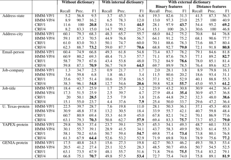
The results of our baseline experiments are shown in Table 2. Since many of these NER tasks can be learned rather well regardless of the feature set used, given enough data, in the table the learners are trained with only 10% of the available data, with the remainder used for testing. (We will later show results with other training set sizes.) All results reported are averaged over 7 random selections of disjoint training and test examples, and we measure accuracy in terms of the correctness of the entire extracted entity (i.e., partial extraction gets no credit).
Without dictionary With internal dictioanry With external dictionary
Binary features Distance features
Recall Prec. F1 Recall Prec. F1 Recall Prec. F1 Recall Prec. F1
Address-state HMM-VP/1 5.2 56.8 9.5 3.7 45.3 6.8 19.3 82.6 31.3 41.5 87.3 56.3 HMM-VP/4 8.9 90.7 16.2 6.5 78.3 12.0 13.0 97.3 23.0 25.7 100 40.9 CRF/1 11.6 100 20.8 31.6 75.1 44.5 28.1 97.9 43.7 54.4 95.2 69.2 CRF/4 8.2 83.3 15.0 14.7 90.2 25.4 15.1 100 26.3 30.6 100 46.8 Address-city HMM-VP/1 60.1 79.3 68.3 48.3 65.7 55.7 68.0 84.2 75.2 70.8 84 76.8 HMM-VP/4 59.1 87.3 70.5 44.9 76.8 56.7 64.1 91.2 75.2 68.1 90.6 77.7 CRF/1 61.0 83.0 70.3 50.1 74.7 60.0 70.1 88.6 78.3 73.6 88.7 80.4 CRF/4 62.3 88.7 73.2 59.0 87.7 70.6 68.8 92.7 79.0 72.1 91.8 80.8 Email-person HMM-VP/1 60.4 74.9 66.8 49.3 61.8 54.8 73.4 83.7 78.2 79.1 84.6 81.8 HMM-VP/4 60.9 80.2 69.3 48.4 71.3 57.7 71.1 87.6 78.5 77.1 89.2 82.7 CRF/1 58.7 79.7 67.6 43.4 53.8 48.0 73.2 84.9 78.6 78.0 85.1 81.4 CRF/4 59.8 87.1 70.9 56.7 74.9 64.5 69.7 89.9 78.5 76.4 89.6 82.5 Job-company HMM-VP/1 1.3 34.7 2.5 0.9 21.7 1.7 2.0 28.1 3.8 8.9 79.8 16.1 HMM-VP/4 3.6 59.8 6.8 1.8 46.1 3.4 11.5 80.6 20.2 18.6 93.4 31.1 CRF/1 35.6 92.7 51.4 10.6 37.8 16.5 37.1 92.2 52.9 40.1 88.8 55.3 CRF/4 38.3 96.1 54.8 12.7 54.6 20.6 39.8 92.8 55.7 45.0 95.5 61.2 Job-title HMM-VP/1 18.4 43.7 25.9 1.7 25.7 3.2 23.9 43.2 30.8 30.9 44.2 36.4 HMM-VP/4 17.3 51.5 25.9 2.5 39.7 4.7 27.9 48.4 35.4 30.9 45.7 36.8 CRF/1 20 50.1 28.5 2.5 7.9 3.8 21.6 44.8 29.2 32.3 48.0 38.6 CRF/4 15.1 55.0 23.7 4.4 37.6 7.9 25.4 50.0 33.7 29.6 47.2 36.4 U. Texas-protein HMM-VP/1 22.5 39.7 28.7 7.6 19.8 11.0 28.1 50.3 36.1 37.1 45.3 40.8 HMM-VP/4 30.9 48.8 37.8 13.2 30.5 18.4 33.9 55.7 42.1 40.7 59.8 48.4 CRF/1 60.7 80.9 69.4 35.3 61.9 45.0 67.8 82.1 74.2 70.1 86.9 77.6 CRF/4 63.1 79.3 70.3 50.8 62.7 57.9 69.4 83.3 75.7 73.7 85.2 79.0 YAPEX-protein HMM-VP/1 29.8 50.3 37.4 23.7 39.1 29.5 45.3 54.1 49.3 48.7 60.1 53.8 HMM-VP/4 30.1 55.7 39.1 28.9 41.5 34.1 43.7 58.3 49.9 50.3 61.4 55.3 CRF/1 58.1 70.2 63.6 50.7 59.4 54.7 69.8 77.4 73.4 73.8 80.1 76.8 CRF/4 61.3 67.9 64.4 52.6 53.2 52.9 71.9 69.8 70.8 78.9 75.6 77.2 GENIA-protein HMM-VP/1 17.5 40.8 24.5 15.6 27.3 19.8 42.7 50.3 46.2 49.3 58.3 53.4 HMM-VP/4 20.5 41.2 27.4 25.1 32.5 28.3 48.5 50.7 49.6 50.7 54.5 52.5 CRF/1 63.1 73.5 67.9 48.1 55.7 51.6 71.8 79.6 75.5 75.4 83.2 79.1 CRF/4 66.8 75.1 70.7 49.8 57.5 53.4 72.7 75.4 74.0 75.8 89.1 81.9
Table 2: Performance of baseline algorithms on eight IE tasks under three conditions: with no external dictionary; with an external dictionary and binary features; with an external dictionary and distance features; with an internal dictionary.
We compared the baseline algorithms on the six different tasks, without an external dictionary (first column), with an internal dictionary (second column), with an external dictionary with binary features (third column), and with an external dictionary with distance features (fourth column). For each we report recall, precision and F1 values4. We make the following observations
concerning the results of Table 2.
• When internal dictionary features are used, the performance of HMM-VP/1, HMM-VP/4, CRF/1and CRF/4tends to drop perhaps because these features are less natural for the Markov models.
• Generally speaking, HMM-VP/4 outperforms or equals HMM-VP/1 and so does CRF/4 over CRF/1.
• Binary dictionary features are helpful, but distance-based dictionary features are more helpful.
• Internal dictionary is unreliable in Markov case. 4.3.2 Performance of SMMs over Best Baseline Algorithms
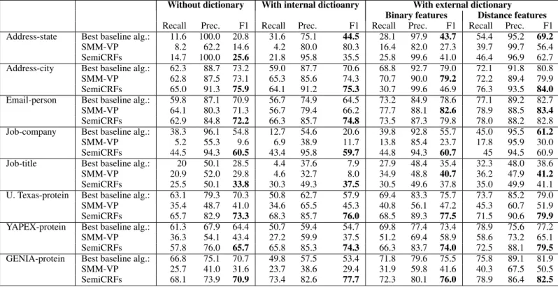
The performance of SMMs is summarized in Table 3. We make the following observations concerning the results of Table 3.
Without dictionary With internal dictioanry With external dictionary Binary features Distance features
Recall Prec. F1 Recall Prec. F1 Recall Prec. F1 Recall Prec. F1 Address-state Best baseline alg.: 11.6 100.0 20.8 31.6 75.1 44.5 28.1 97.9 43.7 54.4 95.2 69.2
SMM-VP 8.2 62.2 14.6 4.2 80.0 80.3 16.4 82.0 27.3 39.7 99.7 56.4
SemiCRFs 14.7 100.0 25.6 21.8 95.8 35.5 25.8 99.6 41.0 46.4 96.9 62.7
Address-city Best baseline alg.: 62.3 88.7 73.2 59.0 87.7 70.6 68.8 92.7 79.0 72.1 91.8 80.8
SMM-VP 62.8 87.5 73.1 65.3 85.6 74.3 70.7 90.0 79.2 72.2 89.4 79.9
SemiCRFs 65.0 91.3 75.9 64.1 91.2 75.3 30.7 99.6 46.9 76.3 93.5 84.0
Email-person Best baseline alg.: 59.8 87.1 70.9 56.7 74.9 64.5 73.2 84.9 78.6 77.1 89.2 82.7
SMM-VP 64.1 80.3 71.3 56.7 79.4 66.2 77.7 88.1 82.6 78.9 88.5 83.4
SemiCRFs 62.9 84.8 72.2 66.3 85.7 74.8 73.5 87.3 79.8 78.0 88.2 82.8
Job-company Best baseline alg.: 38.3 96.1 54.8 12.7 54.6 20.6 39.8 92.8 55.7 45.0 95.5 61.2
SMM-VP 5.2 55.3 9.6 6.9 38.9 11.7 13.8 85.4 23.7 17.8 95.9 30.0
SemiCRFs 44.5 94.3 60.5 43.4 95.8 59.7 44.8 94.3 60.7 45 94.5 60.9
Job-title Best baseline alg.: 20 50.1 28.5 4.4 37.6 7.9 27.9 48.4 35.4 32.3 48.0 38.6
SMM-VP 20.9 52.0 29.8 4.6 32.7 8.0 34.9 48.8 40.7 36.2 47.9 41.2
SemiCRFs 25.5 50.1 33.8 30.3 49.3 37.5 30.5 49.6 37.8 35.0 49.9 41.1
U. Texas-protein Best baseline alg.: 63.1 79.3 70.3 50.8 62.7 57.9 69.4 83.3 75.7 73.7 85.2 79.0
SMM-VP 35.4 48.7 41.0 34.6 65.5 45.3 40.8 56.1 47.2 45.3 60.7 51.9
SemiCRFs 65.7 82.9 73.3 68.3 85.7 76.0 68.5 89.3 77.5 71.5 90.6 79.9
YAPEX-protein Best baseline alg.: 61.3 67.9 64.4 50.7 59.4 54.7 69.8 77.4 73.4 78.9 75.6 77.2
SMM-VP 36.3 54.1 43.4 27.2 59.9 37.5 51.2 69.4 58.9 58.6 73.2 65.1
SemiCRFs 57.8 76.0 65.7 65.8 85.3 74.3 66.3 83.7 74.0 72.5 88.1 79.5
GENIA-protein Best baseline alg.: 66.8 75.1 70.7 49.8 57.5 53.4 71.8 79.6 75.5 75.8 89.1 81.9
SMM-VP 25.7 41.0 31.6 23.7 38.6 29.4 31.9 59.8 41.6 40.3 67.5 50.5
SemiCRFs 68.1 73.9 70.9 73.4 82.6 77.7 72.3 80.1 76.0 78.9 86.4 82.5
Table 3: Comparing performance of best baseline algorithm and SMMs on eight IE tasks under three conditions: with no external dictionary; with an external dictionary and binary features; with an external dictionary and distance features; with an internal dictionary.
• Generally speaking, semi-CRF is the best-performing method. Without an external dictionary, SMM-VP does better than the best baseline algorithm 6 out of 16 times, semiCRFs beat the best baseline algorithm 15 out of 16 times. With an external dictionary, SMM-VP does better than the best baseline algorithm 5 out of 16 times, semiCRFs beat the best baseline algorithm 6 out of 16 times.
• SMMs achieved competitive performance compared to the best published results on the protein name extraction tasks. Bunescu et al. reported an F1 of 57.9 for the dataset from University of Texas [37]. Kazama reported an F1 of 56.5 for GENIA dataset [21]. Franzen et al. reported an F1 of 67.1 for YAPEX dataset[24].
• Internal dictionaries usually improve the performance in the semi-Markov case.
• External dictionaries with distance features help all the models. 4.3.3 Comparison between HMM-VP/4 and SMM-VP
Below, we will perform a more detailed comparison of SMM-VP and HMM-VP/4 under various conditions. We focus on com-paring the F1 performance of SMM-VP and HMM-VP/4 with distance features. We will not present any detailed comparisons of running times of the two methods since our implementation is not yet optimized for running time. (As implemented, the SMM-VP method is 3-5 times slower than HMM-VP/4, because of the more expensive distance features and the expanded Viterbi search.)
Effect of Extensions to Collins’ Method
Table 4 compares the F1 performance of (our implementation of) Collins’ original method (Equation 10, labeled Collins) to our variant (Equation 12, labeled C & S for the segment extension of Collins’ method). We also compare the natural semi-Markov extension of Collins’ method to SMM-VP. In both cases Collins’ method performs much better on one of the five problems, but worse on the remaining four. The changes in performance associated with our extension seem to affect both the Markovian and
Address Email Job State City Person Co. Title
HMM-VP/4 Collins 34.6 76.3 74.9 56.1 32.5
C & S 40.9 77.7 82.7 31.1 36.8
SMM-VP Collins 49.1 78.2 78.1 53.0 33.9
C & S 56.4 79.9 83.4 30.0 41.2
Table 4: F1 performance of the voted perceptron variant considered herevsthe method described by Collins.
0.05 0.1 0.15 0.2 0.25 0.3 0.35 0.4 0.45 -20 -10 0 10 20 30 40 50 60 70 80 90
Fraction of available training data
F 1 s p a n a c c u ra c y Address_State HMM-VP/4 SMM-VP+int HMM-VP/4+dict SMM-VP+int+dict 0.05 0.1 0.15 0.2 0.25 0.3 0.35 0.4 0.45 65 70 75 80 85 90
Fraction of available training data
F 1 s p a n a c c u ra c y Address_City HMM-VP/4 SMM-VP+int HMM-VP/4+dict SMM-VP+int+dict 0.05 0.1 0.15 0.2 0.25 0.3 0.35 0.4 0.45 40 45 50 55 60 65 70 75 80 85 90 95
Fraction of available training data
F 1 s p a n a c c u ra c y Email_Person HMM-VP/4 SMM-VP+int HMM-VP/4+dict SMM-VP+int+dict
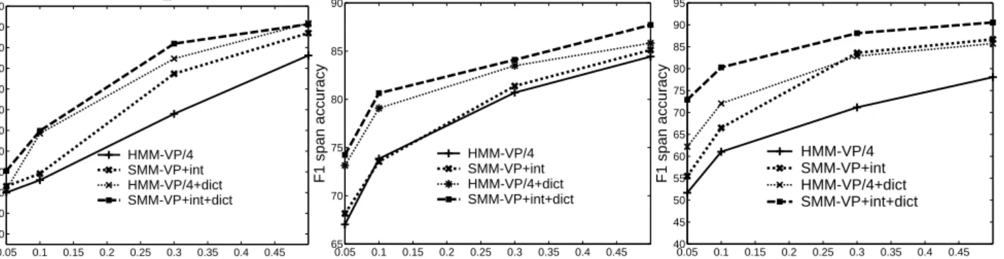
Figure 3: Comparing SMM-VP and HMM-VP/4 with changing training set size on IE tasks from three domains. The X-axis is the fraction of examples used for training and the Y-axis is field-level F1.
semi-Markovian versions of the algorithm similarly. In none of the five tasks does the change from Collins’ original method to our variant change the relative order of the two methods.
Effect of training set size
In Figure 3 we show the impact of increasing training set size on HMM-VP/4 and SMM-VP on three representative NER tasks. Often when the training size is small, SMM-VP is much better than HMM-VP/4, but when the training size increases, the gap between the two methods narrows. This suggests that the semi-Markov features are less important when large amounts of training data are available. However, the amount of data needed for the two methods to converge varies substantially, as is illustrated by the curves for address-city and email-person.
Effect of history size
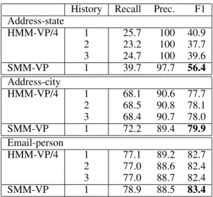
It is straightforward to extend the algorithms of this paper so that HMM-VP/4 can construct features that rely on the last several predicted classes, instead of only the last class. Table 7 we show the result of increasing the “history size” for HMM-VP/4 from one to three. We find that the performance of HMM-VP/4 does not improve much with increasing history size, and in particular, that increasing history size does not change the relative ordering of HMM-VP/4 and SMM-VP. This result supports the claim, made in Section 2.2, that a SMM-VP with segment length bounded byLis quite different from an order-LHMM. Alternative dictionaries
We re-ran two of our extraction problems on alternative dictionaries to study sensitivity to dictionary quality. For emails we used a dictionary of 16623 student names, obtained from students at universities across the country as part of the RosterFinder project [48]. For the job-title extraction task, we obtained a dictionary of 159 job titles in California from a software jobs website5. Recall that the original email dictionary contained the names of the people who sent the emails, and the original
dictionary for the Austin-area job postings was for jobs in the Austin area.
History Recall Prec. F1 Address-state HMM-VP/4 1 25.7 100 40.9 2 23.2 100 37.7 3 24.7 100 39.6 SMM-VP 1 39.7 97.7 56.4 Address-city HMM-VP/4 1 68.1 90.6 77.7 2 68.5 90.8 78.1 3 68.4 90.7 78.0 SMM-VP 1 72.2 89.4 79.9 Email-person HMM-VP/4 1 77.1 89.2 82.7 2 77.0 88.6 82.4 3 77.0 88.7 82.4 SMM-VP 1 78.9 88.5 83.4
Table 5: Effect of increasing history size of HMM-VP/4 on F1 performance, compared to F1 performance of SMM-VP.
Recall Prec. F1 Recall Prec. F1 Recall Prec. F1
Email-person No dictionary Original dictionary Student names
Dictionary lookup 43.11 85.3 57.3 0 0 0
HMM-VP/4 60.9 80.2 69.3 77.1 89.2 82.7 73.5 86.3 79.4
SMM-VP 64.1 80.3 71.3 78.9 88.5 83.4 74.8 84.6 79.4
Job-title No dictionary Original (Austin job titles) California job titles
Dictionary lookup 29.4 29.5 29.4 4.3 27.0 7.2
HMM-VP/4 17.3 51.5 25.9 30.9 45.7 36.8 26.8 47.5 34.3
SMM-VP 20.9 52.0 29.8 36.2 47.9 41.2 36.0 51.9 42.5
Table 6: Results with changing dictionary.
Table 6 shows the result, for HMM-VP/4 and SMM-VP with distance features. Both methods seem fairly robust to using dictionaries of less-related entities. Although the quality of extractions is lowered for both methods in three of the four cases, the performance changes are not large.
4.3.4 Compasison between SemiCRFs and CRFs Effect of training set size
Figure 4 shows F1 values plotted against training set size for a subset of three of the tasks, and four of the learning methods. As the curves show, performance differences are often smaller with more training data. Gaussian priors were used for all algorithms, and for semi-CRFs, a fixed value ofLwas chosen for each dataset based on observed entity lengths. This ranged between 4 and 6 for the different datasets.
Comparison between semi-CRF and order-LCRFs
We also compared semi-CRF to order-LCRFs, with various values ofL.6 In Table 7 we show the result forL= 1,L= 2,
andL= 3, compared to semi-CRF. For these tasks, the performance of CRF/4 and CRF/1 does not seem to improve much by simply increasing order.
0 10 20 30 40 50 60 70 80 90 100 0.05 0.1 0.15 0.2 0.25 0.3 0.35 0.4 0.45 0.5 F1 span accuracy
Fraction of available training data Address_State CRF/4 SemiCRF+int CRF/4+dict SemiCRF+int+dict 65 70 75 80 85 90 0.05 0.1 0.15 0.2 0.25 0.3 0.35 0.4 0.45 0.5 F1 span accuracy
Fraction of available training data Address_City CRF/4 SemiCRF+int CRF/4+dict SemiCRF+int+dict 65 70 75 80 85 90 0.05 0.1 0.15 0.2 0.25 0.3 0.35 0.4 0.45 0.5 F1 span accuracy
Fraction of available training data Email_Person
CRF/4 SemiCRF+int CRF/4+dict SemiCRF+int+dict
Figure 4:F1 as a function of training set size. Algorithms marked with “+dict” include external dictionary features, and algorithms marked with “+int” include internal dictionary features. We do not use internal dictionary features for CRF/4 since they lead to reduced accuracy.
CRF/1 CRF/4 semi-CRF
L= 1 L= 2 L= 3 L= 1 L= 2 L= 3
Address State 20.8 20.1 19.2 15.0 16.4 16.4 25.6
Address City 70.3 71.0 71.2 73.2 73.9 73.7 75.9
Email persons 67.6 63.7 66.7 70.9 70.7 70.4 72.2
Table 7:F1 values for different order CRFs
5 Related work
Besides the methods described in Section 4.1 for integrating a dictionary with NER systems [5, 7], a number of other techniques have been proposed for using dictionary information in extraction.
A method of incorporating an external dictionary for generative models like HMMs is proposed in [43, 4]. Here a dictionary was treated as a collection of training examples of emissions for the state which recognizes the corresponding entity: for instance, a dictionary of person names would be treated as example emissions of a “person name” state. This method suffers from a number of drawbacks: there is no obvious way to apply it in a conditional setting; it is highly sensitive to misspellings within a token; and when the dictionary is too large or too different from the training text, it may degrade performance.
In the work in [53], a scheme is proposed for compiling a dictionary into a very large HMM in which emission and transition probabilities are highly constrained, so that the HMM has very few free parameters. This approach suffers from many of the limitations described above, but may be useful when training data is limited.
Krauthammeret al[27] describe an edit-distance based scheme for finding partial matches to dictionary entries in text. Their scheme uses BLAST (a high-performance tool designed for DNA and protein sequence comparisons) to do the edit distance computations. However, there is no obvious way of combining edit-distance information with other informative features, as there is in our model. In experimental studies, pure edit-distance based metrics are often not the best performers in matching names [11]; this suggests that it may be advantageous in NER to be able to exploit other types of distance metrics as well as edit distance.
Some early NER systems used a “sliding windows” approach to extraction, in which all wordn-grams were classified as “entities” or “non-entities” (fornof some bounded size) (e.g., [17]). Such systems can easily be extended to make use of dictionary-based features. However, in prior experimental comparisons, sliding-window NER system have usually proved inferior to HMM-like NER systems. Sliding window approaches also have the disadvantage that they may extract entities that overlap.
Another mechanism of exploiting a dictionary is to use it to bootstrap a search for extraction patterns from unlabeled data [1, 13, 14, 40, 51]. In these systems, dictionary entries are matched on unlabeled instances to provide “seed” positive examples, which are then used to learn extraction patterns that provide additional entries to the dictionary. These extraction systems are mostly rule-based (with some exceptions [13, 14]), and appear to assume a relatively clean set of extracted entities. In contrast our focus is probabilistic models and the incorporation of large noisy dictionaries.
Another approach of exploiting an “internal dictionary” is the skip-chain CRFs which makes the boundaries and types of distant segments inter-dependent[45].
Sarawagi introduced a succinct representation of features that are common across overlapping segments and the inference running time is proportional to the number of features [41].
6 Conclusions
In many cases, the ultimate goal of an information extraction process is to answer queries which combine information from structured and unstructured sources. In these applications, NER is successful only to the extent that it finds entity names that can be matched to something in a pre-existing database. However, extending state-of-the-art NER systems by incorporating an external dictionary is difficult. In particular, incorporating information about the similarity of extracted entities to dictionary entries is awkward, because the best NER systems operate by sequentially classifyingwordsas to whether or not they participate in an entity name, while the best similarity measures score entire candidate names.
To correct this mismatch we relax the usual Markov assumptions, and formalize a semi-Markov extraction process. This process is based on sequentially classifyingsegmentsof several adjacent words, rather than single words. A major advantage of semi-Markov models is that they allow features which measure properties of segments, rather than individual elements. For applications like NER and gene-finding [28], these features can be quite natural. It also provides an arguably more natural formulation of the NER problem than sequential word classification. For instance, in the usual formulation, one must design a new set of output tags (and make a corresponding change in the tag-to-entity decoding scheme) to account for distributional differences between words from the beginning of an entity and words elsewhere in an entity. In the semi-Markov formulation, one merely adds new features for entity-beginning words.
We compared our proposed algorithm to some strong baseline NER. The new algorithm is surprisingly effective: on our datasets, it usually outperforms the previous baseline, sometimes dramatically.
Acknowledgments
The preparation of this paper was supported in part funded by grants from the Information Processing Technology Office (IPTO) of the Defense Advanced Research Projects Agency (DARPA), as well as National Science Foundation Grant No. EIA-0131884 to the National Institute of Statistical Sciences, and a contract from the Army Research Office to the Center for Computer and Communications Security (CyLab) at Carnegie Mellon University.
Appendix
Implementations of semi-Markov Models are available at http://crf.sourceforge.net, and a NER package using this package is available on http://minorthird.sourceforge.net.
References
[1] E. Agichtein and L. Gravano. Snowball: Extracting relations from large plaintext collections. InProceedings of the 5th ACM Interna-tional Conference on Digital Libraries, 2000.
[2] Y. Altun, I. Tsochantaridis, and T. Hofmann. Hidden Markov support vector machines. InProceedings of the 20th International Conference on Machine Learning (ICML), 2003.
[3] D. M. Bikel, R. L. Schwartz, and R. M. Weischedel. An algorithm that learns what’s in a name.Machine Learning, 34:211–231, 1999. [4] V. R. Borkar, K. Deshmukh, and S. Sarawagi. Automatic text segmentation for extracting structured records. InProc. ACM SIGMOD
International Conf. on Management of Data, Santa Barabara,USA, 2001.
[5] A. Borthwick, J. Sterling, E. Agichtein, and R. Grishman. Exploiting diverse knowledge sources via maximum entropy in named entity recognition. InSixth Workshop on Very Large Corpora New Brunswick, New Jersey. Association for Computational Linguistics., 1998. [6] R. Bunescu, R. Ge, R. J. Kate, E. M. Marcotte, R. J. Mooney, A. K. Ramani, and Y. W. Wong. Learning to extract proteins and their
interactions from medline abstracts. Available from http://www.cs.utexas.edu/users/ml/publication/ie.html, 2002.
[7] R. Bunescu, R. Ge, R. J. Mooney, E. Marcotte, and A. K. Ramani. Extracting gene and protein names from biomedical abstracts. Unpublished Technical Note, Available from http://www.cs.utexas.edu/users/ml/publication/ie.html, 2002.
[8] R. Bunescu and R. J. Mooney. Relational markov networks for collective information extraction. InProceedings of the ICML-2004 Workshop on Statistical Relational Learning (SRL-2004), Banff, Canada, 2004.
[9] M. E. Califf and R. J. Mooney. Bottom-up relational learning of pattern matching rules for information extraction.Journal of Machine Learning Research, 4:177–210, 2003.
[10] W. W. Cohen and P. Ravikumar. Secondstring: An open-source java toolkit of approximate string-matching techniques. Project web page, http://secondstring.sourceforge.net, 2003.
[11] W. W. Cohen, P. Ravikumar, and S. E. Fienberg. A comparison of string distance metrics for name-matching tasks. InProceedings of the IJCAI-2003 Workshop on Information Integration on the Web (IIWeb-03), 2003.
[12] M. Collins. Discriminative training methods for hidden Markov models: Theory and experiments with perceptron algorithms. In
Empirical Methods in Natural Language Processing (EMNLP), 2002.
[13] M. Collins and Y. Singer. Unsupervised models for named entity classification. InProceedings of the Joint SIGDAT Conference on Empirical Methods in Natural Language Processing and Very Large Corpora (EMNLP99), College Park, MD, 1999.
[14] M. Craven and J. Kumlien. Constructing biological knowledge bases by extracting information from text sources. InProceedings of the 7th International Conference on Intelligent Systems for Molecular Biology (ISMB-99), pages 77–86. AAAI Press, 1999.
[15] C. M. R. R. D. Heckerman, D. M. Chickering and C. M. Kadie. Dependency networks for inference, collaborative filtering, and data visualization.Journal of Machine Learning Research, 1, 2000.
[16] R. Durban, S. R. Eddy, A. Krogh, and G. Mitchison.Biological sequence analysis - Probabilistic models of proteins and nucleic acids. Cambridge University Press, Cambridge, 1998.
[17] D. Freitag. Multistrategy learning for information extraction. InProceedings of the Fifteenth International Conference on Machine Learning. Morgan Kaufmann, 1998.
[18] X. Ge.Segmental Semi-Markov Models and Applications to Sequence Analysis. PhD thesis, University of California, Irvine, December 2002.
[19] D. Hanisch, J. Fluck, H. Mevissen, and R. Zimmer. Playing biology’s name game: identifying protein names in scientific text. InPac Symp Biocomput, pages 403–14, 2003.
[20] K. Humphreys, G. Demetriou, and R. Gaizauskas. Two applications of information extraction to biological science journal articles: Enzyme interactions and protein structures. InProceedings of 2000 the Pacific Symposium on Biocomputing (PSB-2000), pages 502– 513, 2000.
[21] Y. O. J. Kazama, T. Makino and J. Tsujii. Tuning sup-port vector machines for biomedical named entity recogni-tion. InProceedings of the Natural Language Processing in the Biomedical Domain (ACL 2002), Philadelphia, PA, 2002.
[22] J. Janssen and N. Limnios.Semi-Markov Models and Applications. Kluwer Academic, 1999.
[23] D. Jensen and J. Neville. Dependency networks for relational data. InProceedings of 4th IEEE International Conference on Data Mining (ICDM-04), Brighton, UK, 2004.
[24] F. O. L. A. P. L. K. Franzen, G. Eriksson and J. Coster. Protein names and how to find them.International Journal of Medical Informatics special issue on Natural Language Processing in Biomedical Applications, pages 49–61, 2002.
[25] D. Klein and C. D. Manning. Conditional structure versus conditional estimation in nlp models. InWorkshop on Empirical Methods in Natural Language Processing (EMNLP), 2002.
[26] R. E. Kraut, S. R. Fussell, F. J. Lerch, and J. A. Espinosa. Coordination in teams: evidence from a simulated management game. To appear in the Journal of Organizational Behavior, 2005.
[27] M. Krauthammer, A. Rzhetsky, P. Morozov, and C. Friedman. Using blast for identifying gene and protein names in journal articles.
Gene, 259(1-2):245–52, 2000.
[28] A. Krogh. Gene finding: putting the parts together. In M. J. Bishop, editor,Guide to Human Genome Computing, pages 261–274. Academic Press, 2nd edition, 1998.
[29] J. Lafferty, A. McCallum, and F. Pereira. Conditional random fields: Probabilistic models for segmenting and labeling sequence data. InProceedings of the International Conference on Machine Learning (ICML-2001), Williams, MA, 2001.
[30] S. Lawrence, C. L. Giles, and K. Bollacker. Digital libraries and autonomous citation indexing.IEEE Computer, 32(6):67–71, 1999. [31] D. C. Liu and J. Nocedal. On the limited memory BFGS method for large-scale optimization.Mathematic Programming, 45:503–528,
1989.
[32] R. Malouf. A comparison of algorithms for maximum entropy parameter estimation. InProceedings of The Sixth Conference on Natural Language Learning (CoNLL-2002), pages 49–55, 2002.
[33] R. Malouf. Markov models for language-independent named entity recognition. InProceedings of the Sixth Conference on Natural Language Learning (CoNLL-2002), 2002.
[34] A. McCallum, D. Freitag, and F. Pereira. Maximum entropy Markov models for information extraction and segmentation. In Proceed-ings of the International Conference on Machine Learning (ICML-2000), pages 591–598, Palo Alto, CA, 2000.
[35] A. McCallum and W. Li. Early results for named entity recognition with conditional random fields, feature induction and web-enhanced lexicons. InProceedings of The Seventh Conference on Natural Language Learning (CoNLL-2003), Edmonton, Canada, 2003. [36] A. K. McCallum, K. Nigam, J. Rennie, , and K. Seymore. Automating the construction of internet portals with machine learning.
Information Retrieval Journal, 3:127–163, 2000.
[37] R. K. E. M. R. M. A. R. R. Bunescu, R. Ge and Y. W. Wong. Comparative experiments on learning information extractors for proteins and their interactions. Artificial Intelligence in Medicine (Special Issue on Summarization and Information Extraction from Medical Documents), 33(2), 2005.
[38] A. Ratnaparkhi. Learning to parse natural language with maximum entropy models.Machine Learning, 34, 1999. [39] M. Richardson and P. Domingos. Markov logic networks.Machine Learning, 62, 2006.
[40] E. Riloff and R. Jones. Learning Dictionaries for Information Extraction by Multi-level Boot-strapping. InProceedings of the Sixteenth National Conference on Artificial Intelligence, pages 1044–1049, 1999.
[41] S. Sarawagi. Efficient inference on sequence segmentation models. InProceedings of the 23rd International Conference on Machine Learning (ICML06), Pittsburgh, PA, 2006.
[42] S. Sarawagi and A. Bhamidipaty. Interactive deduplication using active learning. InProceedings of the Eighth ACM SIGKDD Interna-tional Conference on Knowledge Discovery and Data Mining, July 23-26, 2002, Edmonton, Alberta, Canada. ACM, 2002.
[43] K. Seymore, A. McCallum, and R. Rosenfeld. Learning Hidden Markov Model structure for information extraction. InPapers from the AAAI-99 Workshop on Machine Learning for Information Extraction, pages 37–42, 1999.
[44] F. Sha and F. Pereira. Shallow parsing with conditional random fields. InProceedings of HLT-NAACL, 2003.
[45] C. Sutton and A. McCallum. Collective segmentation and labeling of distant entities in information extraction. InICML workshop on Statistical Relational Learning, 2004.
[46] R. Sutton, D. Precup, and S. Singh. Between MDPs and semi-MDPs: A framework for temporal abstraction in reinforcement learning.
Artificial Intelligence, 112:181–211, 1999.
[47] R. S. Sutton. Integrated architectures for learning, planning, and reacting based on approximating dynamic programming. In Proceed-ings of the Seventh International Conference on Machine Learning, Austin, Texas, 1990. Morgan Kaufmann.
[48] L. Sweeney. Finding lists of people on the web. Technical Report CMU-CS-03-168, CMU-ISRI-03-104, Carnegie Mellon University School of Computer Science, 2003. Available from http://privacy.cs.cmu.edu/dataprivacy/projects/rosterfinder/.
[49] B. Taskar, P. Abbeel, and D. Koller. Discriminative probabilistic models for relational data. InProceedings of Eighteenth Conference on Uncertainty in Artificial Intelligence (UAI02), Edmonton, Canada, 2002.
[50] W. E. Winkler. Matching and record linkage. InBusiness Survey methods. Wiley, 1995.
[51] R. Y. Winston Lin and R. Grishman. Bootstrapped learning of semantic classes from positive and negative examples. InProceedings of the ICML Workshop on The Continuum from Labeled to Unlabeled Data, Washington, D.C, August 2003.
[52] D. H. Wolpert. Stacked generalization.Neural Networks, 5:241–259, 1992.