MODELING DNN AS HUMAN
LEARNER
By
Junrui Ni
Senior Thesis in Computer Engineering
University of Illinois at Urbana-Champaign
Advisor: Prof. Hasegawa-Johnson
Abstract
In previous experiments, human listeners demonstrated that they had the ability to adapt to unheard, ambiguous phonemes after some initial, relatively short exposures. At the same time, previous work in the speech community has shown that pre-trained deep neural network-based (DNN) ASR systems, like humans, also have the ability to adapt to unseen, ambiguous
phonemes after retuning their parameters on a relatively small set. In the first part of this thesis, the time-course of phoneme category adaptation in a DNN is investigated in more detail. By retuning the DNNs with more and more tokens with ambiguous sounds and comparing
classification accuracy of the ambiguous phonemes in a held-out test across the time-course, we found out that DNNs, like human listeners, also demonstrated fast adaptation: the accuracy curves were step-like in almost all cases, showing very little adaptation after seeing only one (out of ten) training bins.
However, unlike our experimental setup mentioned above, in a typical lexically-guided
perceptual learning experiment, listeners are trained with individual words instead of individual phones, and thus to truly model such a scenario, we would require a model that could take the context of a whole utterance into account. Traditional speech recognition systems accomplish this through the use of hidden Markov models (HMM) and WFST decoding. In recent years, bidirectional long short-term memory (Bi-LSTM) trained under connectionist temporal
classification (CTC) criterion has also attracted much attention. In the second part of this thesis, previous experiments on ambiguous phoneme recognition were carried out again on a new Bi-LSTM model, and phonetic transcriptions of words ending with ambiguous phonemes were used as training targets, instead of individual sounds that consisted of a single phoneme. We found out that despite the vastly different architecture, the new model showed highly similar behavior in terms of classification rate over the time course of incremental retuning. This indicated that ambiguous phonemes in a continuous context could also be quickly adapted by neural network-based models.
In the last part of this thesis, our pre-trained Dutch Bi-LSTM from the previous part was treated as a Dutch second language learner and was asked to transcribe English utterances in a self-adaptation scheme. In other words, we used the Dutch model to generate phonetic
transcriptions directly and retune the model on the transcriptions it generated, although ground truth transcriptions were used to choose a subset of all self-labeled transcriptions.
Self-adaptation is of interest as a model of human second language learning, but also has great practical engineering value, e.g., it could be used to adapt speech recognition to a low-resource language. We investigated two ways to improve the adaptation scheme, with the first being multi-task learning with articulatory feature detection during training the model on Dutch and self-labeled adaptation, and the second being first letting the model adapt to isolated short words before feeding it with longer utterances.
Subject Keywords: Phoneme Category Adaptation, Human Perceptual Learning, Deep Neural Networks, Time-course, Long Short-Term Memory, Connectionist Temporal Classification, Second Language Learning, Articulatory Feature Detection, Multi-Task Learning, Semi-Supervised Learning
Acknowledgments
This thesis was co-advised by Prof. Scharenborg at the Delft University of Technology. The author would like to thank her for providing the retuning set and for her help with getting the forced alignment. The author would also like to thank her for all the insights and guidance she provided during all the experiments.
Contents
1. Introduction ... 1
1.1 The Time-Course of Phoneme Category Adaptation in Deep Neural Networks ... 1
1.2 Phoneme Category Adaptation Using Bi-LSTM and CTC ... 2
1.3 Second Language Learner Adaptation ... 3
2. Literature Review ... 5
2.1 Human Perceptual Learning ... 5
2.2 Second Language Learner ... 8
2.2.1 Perceptual Assimilation Model ... 8
2.2.2 Speech Learning Model ... 9
2.2.3 Native Language Magnet ...11
2.3 Neural Network in Speech Recognition ...12
2.3.1 Neural Networks and Back-Propagation ...12
2.3.2 Convolutional Neural Networks ...14
2.3.3 Recurrent Neural Networks, GRU and LSTM...15
2.3.4 Deep Neural Network in Speech Recognition ...17
2.4 Visualization ...20
2.4.1 Principal Component Analysis ...21
2.4.2 Non-negative Factor Analysis ...23
3. Methodology ...26
3.1 Investigating the Time Course of DNN Perceptual Learning ...26
3.2 Investigating the Time Course of Bi-LSTM Perceptual Learning ...29
3.3 Modeling the Dutch ASR Model as a Second Language Learner ...30
4. Experimental Results ...34
4.1 Classification Rates For DNN Perceptual Learning ...34
4.2 Inter-category Distance Ratio For DNN Perceptual Learning ...36
4.3 Investigating Step-like Behavior For DNN Perceptual Learning ...38
4.5 Recognition Rate for Bi-LSTM Perceptual Learning ...50
4.6 Visualizing Phoneme Boundary Shift For Bi-LSTM Perceptual Learning ...52
4.7 Modeling ASR as a Second Language Learner ...62
5. Discussion and Future Work ...67
1. Introduction
1.1 The Time-Course of Phoneme Category Adaptation in
Deep Neural Networks
When encountering a new speaker, both humans and speech recognition systems face the challenge of adapting to the pronunciation of that speaker and must do so in a way such that the new sounds are included into pre-existing sound categories. This process is defined as
perceptual learning, and here, we focused on how pre-trained deep neural networks deal with perceptual learning of an ambiguous phoneme.
In a typical human lexically-guided perceptual learning experiment, listeners are first exposed to deviant phonemic segments in lexical contexts that constrain their interpretation, after which listeners have to decide on the phoneme categories of several ambiguous sounds on a continuum between two phoneme categories (e.g., [27, 95, 102, 109, 112, 114]). This way the influence of exposure to the deviant sound can be investigated on the phoneme categories in the human brain. In this paradigm [112], two groups of listeners are tested. One group of Dutch listeners was exposed to an ambiguous [l/ɹ] sound in [l]-final words such as appel (Eng: apple; appel is an existing Dutch word, apper is not). Another group of Dutch listeners was exposed to the exact same ambiguous [l/ɹ] sound, but in [ɹ]-final words, e.g., wekker (Eng: alarm clock; wekker is a Dutch word, wekkel is not). After exposure to words containing the [l/ɹ], both groups of listeners were tested on multiple steps from the same continuum of [l/ɹ] ambiguous sounds from more [l]-like sounds to more [ɹ]-like sounds. For each of these steps, they had to indicate whether the heard sound was an [l] or an [ɹ]. Percentage [ɹ] responses for the continuum of ambiguous sounds were measured and compared for the two groups of listeners. Lexically-guided perceptual learning shows itself as significantly more [ɹ] responses for the listeners who were exposed to the ambiguous sound in [ɹ]-final words compared to those who were exposed to the ambiguous sound in [l]-final words. A difference between the groups is interpreted to mean that listeners have retuned their phoneme category boundaries to include the deviant sound into their pre-existing phone category of [ɹ] or [l], respectively.
In previous work, it was shown that deep neural networks (DNNs) can also adapt to ambiguous speech by training on only a few examples of an ambiguous sound, with comparable behavior to humans in a similar setting [113]. However, the minimum amount of instances required for a DNN to adapt to this ambiguous sound remained unknown. Also, it would be useful to compare the time-course between humans and machines during this type of adaptation setting, thus helping to connect human perceptual learning with machine perception. Lastly, while visualizing the weights of DNN still remains an open topic, it would be interesting to show how the weights evolve through time as more adaptation tokens are fed. Therefore, the goal of this part of the thesis is three-fold: (1) to investigate the time-course of phoneme category adaptation in a DNN in more detail; (2) to connect between how humans and machines deal with phoneme category
adaptation; (3) to visualize the process of DNN phoneme category adaption over the time-course (by visualizing weights of the neural network).
1.2 Phoneme Category Adaptation Using Bi-LSTM and CTC
The goal of this part is very much the same as the first part, i.e., to observe the time-course of adaption and to visualize the time-course via neural network visualization. The main difference is that we changed the model for a human listener from a multi-layer DNN which is only capable of taking the context information of a fixed number of frames, to an end-to-end Bi-LSTM model that given the utterance of a word, would output the phonetic transcription of the utterance as a whole. Using Bi-LSTM and CTC loss for investigating machine perceptual learning is a better choice for connecting with human perceptual learning, for the following reasons:
1) In a typical human lexically-guided perceptual learning experiment, listeners could almost always refer to lexical contexts to constrain their interpretation [27, 66, 67, 102]. However, as the DNN model proposed previously could only take up to a fixed number of context frames (around 10 frames before and 10 frames after the current frame in our settings), the lexical context is, arguably, completely lost. Even if the training sounds from the re-tuning set were first grouped into words and fed to the DNN word by word, there is no guarantee that a simple multilayer DNN would make use of the contextual information implied by the data order to retune its internal representation. While it would certainly be interesting and useful to investigate how DNN applies “perceptual learning” to individual phonemes, the experimental setup is still not as close to how humans actually perform such adaptation.
2) Bi-LSTM, combined with CTC training and decoding [1, 53, 54], goes directly from raw spectrogram input to a sequence of phonemes (hence the notion of end-to-end model). Due to the use of input/output/forget gate, memory cell [49, 59] and bidirectional
structure [53], every output unit inside of a Bi-LSTM model could in theory capture all the useful information from a whole input sequence. Note that this would be more similar to human perceptual learning experiments, as humans also hear the whole words, as opposed to individual phonemes, during perceptual learning experiments, and most likely use information from the whole utterance (for example, what the previous phonemes are and so what would the word most likely be) to determine whether the ending ambiguous sound [l/r] should be interpreted as [l] or [r]. Another nice property of the end-to-end Bi-LSTM-CTC model was that the CTC training algorithm is alignment free—it does not require an alignment between input and output sequence, very much like how humans perform adaptation in perceptual learning settings (i.e., they are almost never given a forced alignment of words during the perceptual learning experiments) [27, 66, 67, 102].
1.3 Second Language Learner Adaptation
Human L2 learning has been relatively well studied by three dominant theories (perceptual assimilation model [10, 11, 12, 86], speech learning model [35, 43], and native language magnet model [73]). The details of the three theories are reviewed in the next section, but PAM generally answers the question of why certain non-native phonetic contrasts are better
discriminated than others before learning takes places; SLM investigates why certain L2 phonetic segments are better learned than others over the process of learning; NLM explains the perceptual magnet during infant’s perceptual development.
Therefore, it would be interesting to ask how a machine (in this case, a deep neural network-based speech recognizer) would try to “learn” a second language, and how its performance could be improved via specific techniques used in human second language teaching. Here the word “learning” is restricted to the learning of recognition tasks only, and the performance is measured by phone error rate of the transcription.
ASR systems trained on one specific language usually perform poorly if asked to transcribe a different language, even if those two languages are closely connected [57, 110, 111]. Some difficulties include: (1) Some of the phones in the L2 language are not present in the L1
language, so in order to create those additional units, additional softmax layers must be created [110, 111]; without proper initialization, the recognition rate would be close to chance-like. (2) Even for the shared phonetic units of the two languages, there is little to no guarantee that the same IPA symbol corresponds to the same equivalent class of acoustic features [57]. However, they are mapped to the same softmax unit in the output layer and go through the same set of hidden representation transformations. (3) Recording conditions, speaker variations within cross-lingual data further complicates the issue as neural network-based ASR usually “prefers” input signals that are somewhat similar to the corpus it is trained on.
In the last part of the thesis, we use the self-training paradigm to adapt a relatively well-trained Dutch ASR model for transcribing English utterance. The model used here is similar to the one used in the previous part, i.e. a Bi-LSTM model trained using the CTC criterion. The self-training paradigm incorporates a three-step workflow[110]: 1) in the initialization step, missing L2
(English) phones are added to the softmax layer and initialized using a linear combination of phones in the L1 language (Dutch), based on linguistic knowledge about those phones 2) The initialized model is then asked to transcribe English utterances directly, and phone error rates are calculated using ground truth English phonetic transcriptions 3) Selected percentages (based on error rates) of the self-labeled utterances are used in a subsequent adaptation step to update the model weights.
The subsequent adaptation is capable of creating a statistically “better” model than the
initialized model (see a conservative discussion in [110]); however, the decrease in error rate is still too small to notice any difference during visualization - i.e., a clear adaptation course, in terms of phone recognition rate of individual phones, is too hard to observe from the result. Therefore, two methods to improve the adaptation are proposed:
(1) In PAM, Best mentioned that non-native speech perception is strongly affected by listeners’ knowledge of native phonological equivalent classes, i.e., the articulators [8]. It would be natural to extend the idea to machine L2 learning, i.e., utilizing articulatory feature detection as an auxiliary task for phone transcription. When training the model on Dutch (L1 learning state), the articulatory feature detection units are trained jointly with the phone output layers to implicitly learn an equivalent mapping from phones to sets of articulatory features.
(2) In most early L2 learning classroom settings, students tend to first learn individual words before they move onto longer sets of words or sentences. Analogously, it would be interesting to see if our Bi-LSTM-CTC ASR model would benefit from first adapting isolated words segmented from the adaptation set in the first pass before adapting to connected words and longer sentences in the subsequent pass. Also, as the CTC model is summing up all the possible alignments during the training phase [52], using shorter training utterances (i.e., isolated words) could help the model detect phone boundaries better.
2. Literature Review
The first two parts of the thesis involve how deep neural networks perform the task of lexically-guided perceptual learning in the special case of phoneme category adaptation (after re-tuning on a small set of ambiguous sounds). Therefore, the first section of this literature review will cover human perceptual learning [27, 102, 109].
The third part of the thesis involves how deep neural networks trained on one language could be modeled as a second language learner adapting to a new language. Therefore, in the second section of this literature review, topics on second language learner behavior will be discussed [8, 35, 74].
All speech learning models built throughout the thesis are based on deep neural networks. Therefore, in the third section of this literature review, neural networks and optimization will first receive a general discussion, followed by applications of deep neural networks in speech recognition [1, 52, 53], with an emphasis on the algorithms [52] and models [1] used in this thesis.
2.1 Human Perceptual Learning
In Perceptual learning for speech [109], Samuel and Kraljic reviewed several lines of research under two themes of perceptual learning: with Theme I being the case where the listener's ability to identify unfamiliar speech stimuli (nonnative phonetic contrasts; accented
speech/dialects; degrade speech) improved after experience, and Theme II being the case where the listeners were presented with phonetically ambiguous stimuli and measurement of perceptual learning is more of phonetic boundary shift than of improved comprehension ability. Some of the research in Theme I included discovering improved ability to distinguish between /r/ and /l/ for both bilingual and monolingual native Japanese speakers, after high-variability
training of /r/-/l/ contrast [84], and showed both generalizations in terms of new speakers/tokens [83, 84] (although test subjects were significantly more accurate on familiar talkers [82]) and relatively long-lasting (three to six months as found out by retest) perceptual learning effect on modification to phonetic perception [82]. Moreover, the effects of perceptual learning in the case also enhanced the ability of Japanese speakers to produce the distinction of /r/-/l/ [47] that also showed long-term effects [17]. Similar results apply to native English speakers learning
Mandarin tones (which are considered suprasegmental contrasts), with test subjects showing significantly improved ability in identifying the four tones [121], as well as to Chinese speakers improving their distinction of English contrasts (using either two-alternative forced-choice procedure or same/different discrimination procedure with non-significant differences) [36], suggesting the development of perceptual learning in both cases.
Accented speech can be hard to understand perceptually. Like the experiments in nonnative phonetic contrasts, using a high-variability method to train American listeners on accented speech from native Chinese speakers gave better generalization than the low-variability method, and in the latter case, improved perception could only be observed if training and testing speakers were the same, although the generalization of the former case also failed when another accent was encountered [16]. Further research [22] showed that less extensive training on only more than a dozen sentences (lasting only about one minute) of accented speech was able to improve the perception (instead of developing general strategies to cope with difficulty) of listeners in terms of matching visual targets. In the case of idiolect speech, reviewed research showed that people who were good at talker recognition performed better on speech from familiar talkers, while people who were not good at talker recognition in the first place showed no such difference, indicating speaker-specific learning effects [96], while reviewed research on deaf speech showed that experienced deaf speech listeners were good at recognizing deaf speech under different contexts even if the speaker was newly-encountered [89].
In the case of degraded speech after compression, fast perceptual learning could also be
observed after 5 to 10 training sentences, when sentences were compressed to less than half of their original length [28]. Even more so, subsequent reviewed research showed that knowledge of the language of training sentences did not matter as much and was able to show that
perceptual learning happens at the phonological level (instead of higher levels such as lexical processes) [98]. Experiments with different methods to degrade speech, such as noise
vocoding, showed that hearing a clear version of speech before a vocoded version improved the level of perceptual learning [25]. Also, if nonword vocoded speech stimuli were short enough to retain in phonological STM, the same amount of perceptual learning, in terms of efficacy,
happened as with real word stimuli [58]. As with nonnative phonetic contrast, generalization was also found to be better if vocoded speech came from different speakers (but the results varied as to the amount of misalignment) [118]. Similar perceptual learning results were also obtained with synthesized speech, and sleep between training and testing was found to consolidate the effect of perceptual learning [32].
Theme II of Samuel and Kraljic’s review focused on phonetic retuning. This part of their review is more relevant to establishing the time-course of ambiguous phoneme adaptation experiments carried out in the first and second part of this thesis. Listeners were presented with ambiguous stimuli with context information, and perceptual learning happens as a shift in phoneme
categorization, as listeners started to align the ambiguous phonemes with the context information [109]. In experiments related to lexically induced learning, listeners exposed to ambiguous sounds in the middle of /f/ and /s/ were able to use lexical information, such as whether interpreting that sound as /f/ would result in a real word, to guide their recognition of this ambiguous fricative, and thus in a subsequent categorization test would give more /f/ responses than /s/ (and vice versa) [95]. Even more so, listeners were able to generalize to words outside of the training set, showing adjustments to prelexical representations of fricatives [90], with perceptual learning happening automatically upon just hearing those words with ambiguous sounds (i.e., without explicitly identifying the sound or the word) [91], and such
learning can be quite long-lived and persistent [31, 70]. Also, in the case of training listeners with new “words”, with some of them containing ambiguous fricatives, perceptual learning results were better generated as listeners formed better lexical information about those novel words, under the guide of novel picture association [76]. However, interestingly, the “critical phonemes” in these studies also played a role, as fricatives /s/ and /f/ did not generalize well to new speakers and tend to be speaker-specific [67], while stops such as /d/ and /t/ did generalize (to both new voices and another pair of stops, in particular,/b/-/p/ [66]) and tend to be speaker-general [66, 67]. Other interesting effects of the perceptual system include the fact that the pronunciation of a new speaker was not learned unless they were encountered at the beginning, and that speaker-external factors were also not learned [69]. Several other mentioned
experiments in the review, such as studying the perception of non-ambiguous sounds (which proved that learning is based on dynamic adjustments of the representations of sounds rather than transformation of signal) [24], production (production system did not change after
perceptual learning) [68], and vowel space remapping (which showed very targeted shifts rather than boundary relaxation, and did not incur a complete remap of vowel space) [86] all provided useful aspects on this subject.
One last aspect of the review by Samuel and Kraljic covered audio-visual perceptual learning. Results showed that listeners associated ambiguous sounds with the face they saw articulating that sound (recalibration) [6], and repeated exposure to un-ambiguous sounds with
corresponding articulating faces (selective adaptation) reduced reports of ambiguous sounds as the repeated unambiguous ones [6]. Also, recalibration and selective adaptation showed
different time courses, with a monotonically descending course for selective adaptation, and curvilinear course (a rapid build-up, followed by a plateau, followed by a gradual decline) for recalibration [120].
One important focus of this thesis is on the time-course of perceptual learning, which was studied in detail in the following two papers.
In the paper The Time Course of Perceptual Learning [102], the author fed one group with ambiguous [s/f] sounds in /s/-final words and another group with ambiguous [s/f] sounds in /f/-final words and utilized the visual-world eye-tracking paradigm, with displays that could be used as either training trail or test trial. Their set of stimuli contained the same number (20) of training items where the fricative could only be interpreted as either /s/ or /f/ (not both), temporary minimal pairs where the fricative could be interpreted as both but can be disambiguated using future context, and 20 minimal pairs which did not have any disambiguating context and thus were used for testing. The stimuli were presented in 20 mini-blocks, each consisting of one training item, one contrast item (e.g. natural /s/ for /f/-bias group), both members of a minimal pair (ambiguous fricative + natural contrast item) and one member of a temporal minimal pair. According to the experimental results from eye-tracking distance and fixation time, perceptual learning was found to occur at roughly mini-block 10, which includes 10 training items and 10 [s/f]-bearing temporary minimal pairs.
In the paper Processing and Adaption to Ambiguous Sounds during the Course of Perceptual Learning [27], the authors investigated the perception and processing of words with ambiguous [f/s] sound during the course of lexically-guided perceptual learning and tried to answer whether these ambiguous words were processed as natural stimuli, and what the time course was like. They created stimuli of prime-target pairs, where prime words are /f/ and /s/ final words of either natural sound or ambiguous sound (with a five-step continuum chosen using a pilot test), and target words being words that are semantically related words with neither /f/ or /s/ nor any ambiguity. They performed a lexical decision where listeners decide if the word is a real word with recorded response time, followed by a phonetic categorization task on the five-step /f/-/s/ continuum where listeners decide whether the word ends with /s/ or /f/. Some conclusions include the fact that prime words with ambiguous sounds had a lower acceptance rate than natural words and had a longer response time (with the relationship that primes with lower acceptance rate needing longer processing time) but without affecting the processing of the following target word, as well as that participants exposed to ambiguous /s/ sounds in /s/-final words gave more /s/ responses that ambiguous /f/ sounds in /f/-final words (showing lexically guided perceptual learning). Their most related conclusion to this thesis was that recognition of ambiguous words did become more natural-like towards the end of the exposure, with an increasing acceptance rate. Moreover, this happened after approximately 15 items, showing a step-like manner, which was on par with the results from related literature [66, 67, 102].
2.2 Second Language Learner
Second language learners often have difficulty perceiving the phonetic differences among contrasting consonants or vowels that are not distinct in their native language [51, 104, 119]. Three theoretical frameworks, which are Best’s perceptual assimilation model (PAM), Flege’s speech learning model (SLM), and Kuhl’s Native Language Magnet model (NLM), offer
explanations as to how and why one’s native speech system affects the learning of sounds from a second language. PAM focuses on how non-native contrasts are mapped to native language perceptual space before formal second language learning takes place; SLM focuses on how second language acquisition evolves over time; NLM specifically targets the formation of language-specific pattern during the development of infant’s perceptual space.
2.2.1 Perceptual Assimilation Model
Classic views such as critical early tuning [30] failed to explain why successful contrast tuning could be successful during adulthood [83, 84] and why adult discrimination of nonnative contrasts is not uniformly poor [7, 104]. The fundamental premise of PAM is that non-native segments tend to be perceived according to their similarities to, and discrepancies from, native segments that are closest in the native phonological space [9]. PAM further hypothesizes that non-native contrasts are best discriminated if perceived as phonologically equivalent to a native
contrast, still well discriminated if perceived as phonetic distinctions between good and poor examples of a single native consonant, and much worse if the two non-native contrasts are phonetically equivalent to a single native consonant [8, 9].
PAM is also directly related to articulatory phonology and claimed that non-native speech perception is strongly affected by listeners’ knowledge of native phonological equivalent classes. Non-native phones can be assimilated to native phones based on articulators, constriction locations and/or constriction degrees used [9, 10, 11, 12].
According to [106], a single non-native phone can be assimilated into the native system in three ways: (1) categorized exemplar of native phoneme, (2) uncategorized phoneme that falls between native phonemes, (3) non-assimilable sound with little similarity to any native
phoneme. According to this, several pairwise assimilations of two non-native phones exist: (1) two non-native phones assimilated to two different native phonemes (two category assimilation), (2) two non-native phones assimilated to a single native phoneme (single category assimilation), (3) two non-native phones assimilated to a single native phoneme with different levels of fit (category goodness difference), (4) uncategorized-categorized pair, (5) two uncategorized segments, (6) two non-assimilable sounds.
Therefore, PAM predicts that NA sounds, as unaffected by native phonology, can have good discrimination if the sounds themselves are different enough. TC and UC should also be discriminated well. CG would be well enough if one is a good fit and one is a bad fit but otherwise hindered, and SC would most likely be hindered as well, with the famous /r/-/l/ case for Japanese speakers. UU is affected by non-native contrast similarity and nearby native phones and can range from fair to good [8, 9].
2.2.2 Speech Learning Model
Speech Learning Model tackles the question as to why individuals learn or fail to learn to
accurately perceive and produce phonetic segments in the second language [35]. The research by Flege focused on determining if there are “unlearnable” L2 sounds, and if so, are those sounds limited to adults, as well as how the perception of speech sounds encountered on the phonetic surface of an L2 influence their eventual production.
Some prior research and hypotheses that constitute the development of SLM prior to its formal establishment include, but are not limited to, several hypotheses:
(1) Critical Period Hypothesis (CPH), which, apart from the proposed notion for a critical period for primary language acquisition, also casually included the following claim: past a critical age, it is difficult to learn L2 without a foreign accent (FA) [79].
(2) Contrastive Analysis Hypothesis (CAH), which claimed that the more different the two languages (L1 and L2) get, the greater the difficulty of learning will be [122].
(3) Categorical Perception (CP), which claims for an absence of clearly perceived changes within a category as the stimuli cross a category boundary [107].
However, Flege pointed out through experiments that most of the above early theories
regarding L2 suffered severe flaws. Some examples include: for the critical period hypothesis, a group of immigrants ([34] studied Italians; [46] studied Koreans) with different ages of arrival in North America was tested on their foreign accent, and the results showed that while few subjects with entry age after 12 were without FA, less than half who entered prior to 12 still demonstrated foreign accent [84]. Also, studies on Korean children in North America showed that FA was still detectable after 3-5 years of emergence [37, 84], and thus FA was definitely not the result of passing a critical period. Also, CPH cannot explain why some adult L2 learners manage to speak without FA [15]; for CAH, experiments on different groups of Americans with French experience [45] showed that adult L2 learners can be more successful at producing a “new” vowel sound that was very different from any other sound in the L1 inventory while having difficulty with a similar vowel, which was exactly the opposite of what CAH suggests; for CP, Flege found out that native English monolinguals displayed ability to detect within-category variations of French-accented /tu/. Other research on the commutability of existing abstract phonemic features [40] and learning of new phonemic features [41, 88, 94] further complicate L2 acquisition, as while Arabic learners of English did not recombine existing abstract features to produce a new L2 sound [40], it can be difficult for an L1 speaker to acquire a new, abstract feature in L2 [88], but the difficulty was related to age of learning [41, 94]. Furthermore, learning an L2 was also found to affect the production of L1, and the effects seemed to be stronger for early learners [124].
The SLM was therefore developed to make sense of empirical results that contradicted some earlier theories. Some basic premises of SLM include [35, 43]:
(1) L2 learners can, in time, perceive L2 phonetic properties.
(2) L2 speech learning takes time and is influenced by nature of input (as in L1). (3) L2 production is guided by perceptual representations stored in long-term memory. Further propositions and hypotheses include:
(4) The process and mechanism that guide L1 speech acquisition (such as the ability to form new phonetic categories) remain intact throughout life [44, 45].
(5) The L1 and L2 phonetic elements exist in common phonological space and mutually influence each other [45].
(6) The greater the perceived dissimilarity (as measured in perceptual experiments) of an L2 sound from the closest L1, the more likely a new category will be formed.
(7) Category formation for L2 sound becomes less likely through childhood as representations for neighboring L1 sound develop.
(8) When a category is not formed for L2 sound because it is too similar to an L1 sound, merged L1-L2 takes place.
The implication of (1), (2), (5) and (6) is that at the early stage of L2 learning, L2 vowels that are rated as perceptually similar (as L1 vowels) could be produced quite well, but not those that are
perceptually dissimilar, but over time, the production performance of those dissimilar ones would surpass those similar ones as dissimilar vowels tend to form new categories while those similar will not. While (8) is considered as an implication of (5), another implication is that when categories are created for an L2 vowel, the L2 vowel and its close L1 vowels will try to push apart in the perceptual space to minimize confusion, but that may make the production of one or both sounds less accurate [38].
2.2.3 Native Language Magnet
Infant speech perception and speech production changed from general to language-specific (with respect to the ambient language) after about a year [73, 123]. NLM suggests that linguistic experience alters the perceptual space of speech stimuli, in terms of “magnet effect”, where the most representative instances of a phonetic category function like magnets, attracting nearby members of the same category [72, 73], and therefore makes it difficult to discriminate between the “prototype” and those other sounds [74]. By comparing the adult perception of prototypes and non-prototypes of native and foreign vowels, with those of infants, studies showed that this magnet effect formed as early as 6 months into the infant’s life [71, 72, 103] (and 10 -12 months for consonants [103]). Other studies of the perceptual space using MDS and a synthesized set of syllables at equal distances also showed that perceptual space is distorted and shrunk around the best “representations” while stretched near the category boundary [62].
The formal theory of NLM incorporates three phases of speech development [73, 74]: (1) Phase one refers to the infants’ born abilities to partition sounds into gross categories, separated by natural boundaries, with no dependence on a specific language (i.e., just basic auditory perceptual processing mechanism).
(2) Phase two refers to the perception of a 6-month-old infant. As infants have heard quite an amount of ambient speech, they start to develop different representations of the properties of vowels in their memory, and as their ambient language differs, their representation of the vowel system also differs, and start to show language-specific magnet effects.
(3) Phase three refers to the later stage when magnet effects caused certain acoustic differences to be minimized and others to be maximized, thus erasing some of the natural boundaries that existed in earlier phases, especially those contrasts that are not in their native or ambient language. At this phase, the warped perceptual space starts to take place.
NLM explains how speech perception changes in the infant stage [123] and why adults have certain perceptual behaviors with regard to sounds in a foreign language [10, 33] (for example, it explains Japanese speakers /r/-/l/ difficulty by predicting that their Japanese category prototype will attract both /r/ and /l/ [74]).
2.3 Neural Network in Speech Recognition
2.3.1 Neural Networks and Back-Propagation
Deep neural networks are powerful learning machines made up of rather simple building blocks such as matrix-vector multiplication and scalar nonlinearities [29]. For simplicity, this section will only derive some of the formulas for learning a two-layer network; the algorithm for learning a deep neural network with more than two layers should be rather similar.
Suppose the input vector is of dimension , and denote of dimension as
concatenated with an extra one, used for adding a bias to the output vector . Then the initial output after going through the first layer of the neural net can be written as:
(1)
where is a linear transformation matrix of , and is the dimension of . Note that the extra input dimension effectively adds a bias to the output. The final output from this first hidden layer is obtained after applying an element−wise scalar nonlinear function to , i.e.,
(2)
Some popular non-linear functions for the hidden layer include: a) Sigmoid, denoted as
b) Tanh, denoted as
c) ReLU, denoted as
The second layer of the network takes the output from the previous layer, concatenates with a scalar one again to add bias, and multiplies by a second weight matrix of to get the output vector , i.e.
(3) The final output from this second layer is denoted as
(4)
where denotes the output (nonlinear) function. Some common output functions include sigmoid, which is used for binary classification and softmax:
(5) which is used for multi-class classification.
In order to train a two-layer neural network, we need to optimize its parameters by minimizing some error metrics. For linear outputs, the error is chosen to be the mean squared error between the target and the output , i.e.
For softmax output and one-hot target vectors, the cross-entropy loss is used, i.e. (7)
where are entries of the one-hot target vector , and are the probability outputs for each class from the softmax output layer of the network.
With the loss defined, training the weight matrix and is achieved via gradient descent. Gradient descent is an iterative update algorithm that uses the derivative of the loss function to update the parameters of the model. Suppose and are elements in the two weight matrices in the previous iteration, and and are the weights in the next iteration, then the update formula is:
(8)
where is called the learning rate, which is usually tweaked for best convergence.
To actually obtain the gradient of the loss with respect to and , backpropagation is used, which can be considered as continuously applying chain rule until it reaches the partial
derivative of interest. Therefore, we have
(9) where the second term in the summation comes from the fact that
(10) and thus
(11) The first term is denoted as
(12) which equals to
(13) if cross-entropy loss is used, and equals to
(14)
if mean squared error with nonlinear function is used. To calculate the gradient with respect to the weight matrix of the first layer, the loss is further back-propagated to the first layer, and so we have:
(15) where
2.3.2 Convolutional Neural Networks
Convolutional neural networks (CNNs), which were first proposed in [2] to recognize spatio-temporal bipolar patterns associatively, are now widely applied in computer vision for image classification [117], object detection [106], super-resolution [77], etc. They are also used in speech recognition models for learning temporal and frequency features from spectrograms before feeding into recurrent layers [1]. The filters defined by the convolutional layers try to learn a set of translation-invariant features from the given input [65], thus avoiding hand-crafting various kinds of matched filters.
There are two additional kinds of layers in a CNN, the convolutional layer and pooling layer. Given input , where denotes row dimension out of , denotes column dimension out of , and denotes channel dimension out of , the convolutional layer is defined as a per-channel 2D convolution between and convolution filter set
of size , as:
(17) where is the output feature map from the convolutional layer, with channel size . The output usually goes through some activation function; here for simplicity, only the ReLU function is considered.
Another type of layer is the pooling layer. Here only max-pooling will be discussed; other types of pooling are similar enough. Given the previous post-ReLU activation output, max-pooling is defined as:
(18) with
(19) where is the pooling stride. Note that there are no trainable weights associated with pooling layers.
To train the filters , backpropagation followed by gradient descent is used. Suppose the loss for a single training token is , according to the chain rule, we have
(20) As
(21) It is easy to see that
(22) Therefore, it is easy to get
(23) where
(24)
is the loss back-propagated to the pre-activation output . Note that this is a correlation with respect to back-propagated error and input feature map.
The derivative with respect to can be similarly computed as
(25) which is another correlation, but with respect to back-propagated error and filter weights. Suppose that during backpropagation, the gradient has now been propagated to , then the previous term could be calculated as
(26)
where the last term could be simply calculated as 1 if “survives” the max-pooling and ReLU activation, and 0 otherwise.
2.3.3 Recurrent Neural Networks, GRU and LSTM
The recurrent neural network (RNN) and its variants are widely used in sequence learning tasks such as machine translation [19] and speech recognition [1, 19, 53]. Given an input sequence
, an RNN [53] computes the hidden representations and output vectors iteratively as:
(27) (28)
where is the input weight matrix, is the hidden weight matrix, is the output weight matrix and are bias vectors for hidden representation/output. The function is the hidden activation function, which is usually a sigmoid function [53].
One problem with uni-directional RNNs is that for a time step within the forward pass, that time step could only access information prior to itself, i.e., from to . For speech recognition, it would usually be helpful to gain access from future context as well [23]. Therefore, two separate layers are used in bi-directional RNN [116], one for processing forward sequence and one for processing backward sequence, as follows:
(29) (30) (31)
However, naive RNN structure often suffers from the exploding/vanishing gradient problems [5, 99] and thus possesses little capability of learning long-range contextual information.
Therefore, Long Short-Term Memory (LSTM) units are proposed [49, 59]. A common LSTM unit incorporates a memory cell, an input gate, an output gate and a forget gate [49]. The
architecture permits LSTM to bridge between two input events with a large time lag, relatively independent of the intervening time steps [49]. The formula for calculating the gate values, the cell state, and the hidden representation of an LSTM network [49, 53] is defined as follows:
(32) (33)
(34) (35) (36)
where , , , are the input gate, forget gate, cell state and output gate, respectively. Combining LSTM with bi-directional architecture gives Bi-LSTM [1, 53], which forms the backbone of speech recognition models for the second and third part of this thesis.
Another RNN unit worth mentioning is called Gated-Recurrent Unit (GRU) [20]. Like LSTM, GRU also uses gates to modulate information flow within the unit. It consists of two gates, an update gate and a reset gates, which jointly decide how much of the previous activation and candidate activation should be recorded as the current state. However, unlike LSTM, GRU does not have control of the amount of current state exposed to output [21]. The formula for the forward pass of GRU is defined as:
(38)
(39) where is the update gate vector and is the reset gate vector.
2.3.4 Deep Neural Network in Speech Recognition
One important algorithm that allows recurrent neural networks (RNNs) to learn an end-to-end mapping from raw speech input space (usually spectrogram or Mel-spectrogram) to the label space of phonetic transcription without any pre-segmentation or
post-processing is called Connectionist Temporal Classification (CTC) [52, 54]. It assumes that the target sequence length is at most as long as the input sequence length , and learns a probabilistic distribution over all possible label sequences given the input sequence. The derivations below came from the original CTC paper [52].
The CTC label space consists of one extra label than the label originally in , known as the blank label. This, together with the original labels, allows all possible label alignment with respect to the input sequence. Denote this new set of labels as , then given a specific sequence of softmax output from the RNN, we have
(40)
where is the probability of label at time , and the outputs are conditionally independent. To map from of to the actual transcription of , the many-to-one mapping is used, which removes blank symbols from , and squashes other repeating symbols that are not separated by a blank into one single symbol. Using , the probability of a given labeling of is defined as:
(41) which is the total probability of all paths corresponding to .
The objective function for training the CTC network is again based on maximum likelihood. The CTC Forward-Backward Algorithm offers an efficient way to calculate the probability as follows:
1. First, for a labeling , denote the forward variable as the total probability of at time :
(42)
Using a modified label sequence with blanks added to beginning and end as well as between every two non-blank symbols, and allowing transition only between blank and non-blank labels or between two distinct non-blank labels, initializing and updating can be carried out as:
a. Initialization: (43) (44) (45) b. Update: ; (46) otherwise (47) (48)
2. Similarly, the backward variable can be defined as the total probability of at time :
(49)
and again using the modified , the initialization and update of can be calculated as: c. Initialization: (50) (51) (52) d. Update: (53) otherwise (54) (55) The probability is simply the sum of and .
Maximum likelihood training is carried out by first calculating the derivative with respect to network outputs . Using
(56) we can get
(57) where
(58) and therefore
(59)
The gradient with respect to as well as previous network weights can be derived using backpropagation and is not discussed further here.
There are several ways to decode an utterance given the model. The simplest decoder is called greedy decoder [52], which basically performs over the label set for all time step
. After obtaining the labels for each time step, the many-to-one mapping is used to get rid of blanks and squash repeated alphabet symbols. However, greedy decoding provides no
guarantee that the decoding is optimal. Other CTC decoding methods include prefix-search [54], beam search [55], and WFST-based decoding [92], some of which, during decoding, uses a lexicon and/or a language model [55, 92] to further improve phone error rate/word error rate. One model that uses the CTC criterion is the Deep Speech 2 model [1]. In fact, the Bi-LSTM model trained in this thesis is directly modified from the Deep Speech 2 model, just to constrain the total number of parameters. In this section, the author will only review the model related part of Deep Speech 2 (DS2).
DS2 takes a spectrogram of power normalized audio clips as input features. It then goes through two layers of convolution in both the time and frequency axis (to model both local temporal invariance and spectral variance), each of which is followed by a clipped ReLU function. Usually, in the first convolutional layer, the time dimension is reduced via striding. Following the convolutional layers are stacked bidirectional recurrent layers, with the activation from the forward unit and the backward unit summed before going into the next layer. Upon reaching the last layer, it goes through a softmax output layer that computes a probability for each of the possible outputs. The outputs of the English model in DS2 includes English characters, space, apostrophe and blank symbol for CTC (note that the modified model in this thesis does not use Dutch/English characters but instead IPA phones). As mentioned earlier, the model is trained using CTC loss, which learns a probability distribution over all label sequences.
DS2 incorporates several techniques for improving the model design. First, they applied a special type for Batch Normalization called Sequence-Wise Norm [75]. A normal Batch-Norm [61] operation is defined as an operation to transform the layer output by
(60)
where the mean and variance are taken as the empirical mean and variance, and and are learnable parameters for scaling and shifting, respectively, before feeding into a non-linear activation function. Sequence-wise Batch-Norm computes the mean and variance both over all items in the minibatch and over the length of the input, and in terms of RNN can be defined as:
(61)
The DS2 paper has found out that as much as 12% of improvement could be achieved had this type of Batch-Norm is used.
Another technique is called Sorta-Grad, which deals with varying length sequences during training. Recall that the CTC loss function is defined as
(62)
where is the network output at time , and is its probability output from the network. As the product term shrinks with a larger , DS2 paper argues that the length of the utterance could be used as a heuristic for difficulty, and thus in the first training epoch, should feed the model in increasing order of length.
One last technique worth mentioning is called row convolution, which is applied to unidirectional variants of DS2 models to reach the same level of performance as bidirectional ones. It
assumes that at every time step, a future context matrix
(63)
is used, and thus defines a parameter matrix of the same size . The output of applying to is defined as
(64)
By placing the row convolution above all recurrent layers, the paper claimed to have gotten an even better character error rate than the best bidirectional model on Mandarin data.
2.4 Visualization
Weight visualization of deep neural networks has been a relatively open and active topic across many fields [4, 125]. In this thesis, the author used the same visualization scheme as in [113] to investigate how the decision boundary and clustering behaviors (w.r.t. natural /l/ sounds, natural /r/ sounds and ambiguous [l/r] sounds) change during the time-course of perceptual learning. This visualization scheme first uses a variant of Non-negative Factor Analysis (NFA) [3] for GMM weight decomposition. After necessary normalization, it tries to model the DNN activations for a given phone utterance v as a shift from the mean activation m. The shift itself is modeled as the product of a fat matrix T and a low-dimensional summary vector for the given utterance
w, which in effect captures the most important non-negative variability of the DNN activations [113]. In this step, the matrix T is optimized using all sounds from the phone set in the retuning set, plus the ambiguous sound.
Following the above step, the summary vectors w for phones of interest (i.e. /l/, /r/ and [l/r]) are extracted and projected onto the first three principal axes with the greatest variance using the well-known algorithm called Principal Component Analysis (PCA) [13, 60, 63, 100]. After this
step, the dimensionality of the summary vectors for the sounds of interest are further reduced and could be plotted in a common 3D space, as defined by the first three principal axes. In the following sections, Principal Component Analysis will first be reviewed, followed by Non-negative Factor Analysis.
2.4.1 Principal Component Analysis
Principal Component Analysis (PCA) is widely used for dimensionality reduction, lossy data compression, feature extraction, and data visualization [63]. The derivation below came from [13].
PCA could be formulated as two different problems, with the first being maximum variance formulation and the second being minimum error formulation:
A. Maximum Variance Formulation [13, 60]
Suppose a D-dimensional dataset of size N needs to be projected onto an M-dimensional space where . It is apparent that such a projection needs to capture as much variance of the original dataset as possible.
Suppose M = 1, and the direction of projection is specified by the vector in the D-dimensional space. Without loss of generality, also suppose
(65)
Therefore, each data point can be projected as a scalar , and the variance could be calculated as
(66) where
(67)
Maximizing with can be done using Lagrange multiplier as the unconstrained maximization of
(68) and setting the derivative w.r.t to zero yields
(69)
so is an eigenvector of with eigenvalue . Left multiplying by yields (70)
and so needs to be the eigenvector with the largest eigenvalue to maximize the variance on the first projected axis.
For M > 1, the principal axes could be incrementally chosen as the eigenvector with the M-th largest eigenvalue in order to maximize total capture variance. To prove this is true,
suppose this holds for , and now needs to be determined. It is obvious that this new vector needs to be orthogonal to the previous principal axes, and so
(71)
It is also obvious that the added variance needs to be maximized in order for the total captured variance to be maximized (as the invariant states that captures the
maximum possible variance for an (M - 1) - dimensional space). Therefore, using Lagrange multipliers, we have
(72) Setting the derivative w.r.t. to zero yields
(73)
Again, moving the middle term to the left and using the orthogonal constraint gives (74)
Left multiplying by shows that the maximum value is reached by choosing to be the eigenvector that corresponds to the M-th largest eigenvalue.
B. Minimum-error formulation [13, 100]
PCA can also be formulated to minimize the projection error. Suppose again the dataset is of D-dimension. Further, suppose there is an orthogonal set of basis vectors
s.t.
(75) Using this basis,
(76) with the last one using
(77)
Suppose the M-dimensional linear subspace (with minimum projection error) is represented by the first M basis vectors. Then the approximation in the M-dimensional space for each is
(78) and the loss becomes:
(79) Taking the derivative w.r.t. and and setting to zero gives
(80) and
(81) Therefore
(82) and the distortion is now
The solution to minimizing above is achieved by choosing , as the eigenvectors of the covariance matrix s.t the i-th eigenvector has the i-th largest eigenvalue , and so the minimal value of is simply the sum of the smallest eigenvalues.
2.4.2 Non-negative Factor Analysis
Non-negative Factor Analysis (NFA) was first proposed in [100] as a subspace method for GMM weight adaptation, which provided complementary information to GMM mean adaptation (for example, the i-vector framework [26]) for language/dialect recognition. The derivations below came from the original NFA paper [3].
The first concept of NFA is the notion of a Universal Background Model (UBM) [108]. UBM assumes that the utterance matrix:
(84) follows the likelihood function:
(85)
with acoustic vectors and parameters of the GMM specified by . GMM weight adaptation, therefore, attempts to adapt the UBM weights to utterance-dependent weights . The utility function for such weight adaptation resembles the auxiliary function in the E-M algorithm [14] for estimating GMM:
(86)
with being the posterior count of the c-th mixture and is held constant during the
optimization. Because the Gaussian pdfs remain unchanged during optimization, the above utility can be further simplified as
(87)
NFA further assumes that, for a given utterance, each of the could be decomposed as a univariate shift from the UBM weight , and therefore has the form
(88)
where is the c-th row of a subspace matrix of size , and being a summary vector for the utterance that best describes all the (univariable) shifts. The difference between NFA and the more well-known NMF [78] (non-negative matrix factorization) is that the entries of the matrix and the summary vectors are allowed to be negative for NFA, as long as the entries in are not.
Finding the joint subspace matrix and the individual summary vectors involves a two−step iterative optimization similar to E−M. In the first step, is held constant and all are updated. In the second step, all summary vectors for all the utterances are held constant and the shared subspace matrix is updated. The equations corresponding to the two steps in each iteration is listed as below:
First step: Updating for all utterances
Using the assumptions above, the utility function for a single utterance can be rewritten as: (89)
where
(90) and
(91)
Given the non-negative constraint on all the adapted weights , the problem becomes: (92)
Subject to
From the equality constraint, we can get . Here, assume that another constraint is enforced(in the second step), and so the equality constraint disappears as it holds for all . The inequality constraint is satisfied by carefully controlling the step size of update. With constraints relaxed, maximizing the utility w.r.t. becomes the following iterative update:
(93) where
(94) To obtain the initial values for , the following equation is used:
(95)
and is chosen as where is iteratively halved until it satisfies the inequality constraint. Second Step: Updating subspace matrix jointly
As the subspace matrix is shared among all utterances, the utility function for updating is the summation of the utility functions for all utterance s. Therefore, the problem becomes: (96) Subject to where (97)
As the condition is used in the first step to relax the equality constraints there, to update , projected gradient descent needs to be used:
(98) where
(99) and
(100)
To initialize , Principal Component Analysis is used on the matrix formed by the ML estimates of from all utterances.
3. Methodology
3.1 Investigating the Time Course of DNN Perceptual Learning
To mimic the set-up for the human listener experiment, we first trained a DNN on a Dutch speech corpus. To mimic or create a Dutch listener, we first trained a baseline DNN using read speech from the Spoken Dutch Corpus (CGN; [97]). The read speech part of the CGN consists of 551,624 words spoken by 324 unique speakers for a total duration of approximately 64 hours of speech. A forced alignment of the speech material was obtained using a standard Kaldi [105] recipe found online [50]. The speech signal was parameterized using a 64-dimensional vector of log Mel spectral coefficients with a context window of 11 frames, each having a segment length of 25 ms with a 10 ms shift between frames. Per-utterance mean-variance normalization was applied. The CGN training data were split into a training (80% of the full data set), a validation (10%), and a test set (10%) with no overlap in speakers.
We used a simple fully-connected, feed-forward network with five hidden layers, 1024 nodes per layer, with logistic sigmoid nonlinearities as well as batch-normalization and dropout after each layer activation. The output layer was a softmax layer of size 38, corresponding to the number of phonemes that existed in our training labels. The model was trained on CGN for 10 epochs using an Adam optimizer with a learning rate of 0.001. After 10 epochs, we reached a training accuracy of 85% and a validation accuracy of 77% on CGN.
Because we aimed to investigate the DNN’s ability to serve as a model of human perceptual learning, we used the same acoustic stimuli as used in the human perception experiment [112] for retraining the DNN (also referred to as retuning). The retraining material consisted of 200 Dutch words produced by a female Dutch speaker in isolation: 40 words with final [ɹ], 40 words with final [l], and 120 ‘distractor’ words with no [l] and [ɹ]. For the 40 [l]-final words and the 40 [ɹ]-final words, versions also existed in which the [ɹ]-final [l] or [ɹ] was replaced by the ambiguous [l/ɹ] sound. Forced alignments were obtained using a forced aligner for Dutch from the Radboud University. For four words no forced alignment was obtained, leaving 196 words for the experiment.
To mimic the two listener groups from the human perceptual experiment, and to mimic a third group with no exposure to the ambiguous sound (i.e., a baseline group), we used three different configurations of the retuning set:
Amb(iguous)L model: trained on the 118 distractor words, the 39 [ɹ]-final words, and the 39 [l]-final words in which the [l] was replaced by the ambiguous [l/ɹ].
Amb(iguous)R model: trained on the 118 distractor words, the 39 [l]-final words, and the 39 [ɹ]-final words in which the [ɹ] was replaced by the ambiguous [l/ɹ].
Baseline model: trained on all 196 natural words (no ambiguous sounds). This allows us to separate the effects of retuning with versus without the ambiguous sounds.
In order to investigate the time-course of phoneme category adaptation in the DNNs, we used the following procedure. First, the 196 words in the three retuning sets were split into 10 bins of 20 distinct words, except for the last two bins, which each contained only 18 words. In order to be able to compare between the different retuning conditions, the word-to-bin assignments were tied among the three retuning conditions. Each word appeared in only one bin. Each bin
contained: 4 words with final [r] (last bin: 3 words) + 4 words with final [l] (penultimate bin: 3 words) + 12 ‘distractor’ words with no [l] or [r] (last two bins: 11 words). The difference between the retuning conditions is:
AmbL: the final [l] in the 4 [l]-final words were replaced by the ambiguous [l/ɹ] sound. AmbR: the final [ɹ] in the 4 [ɹ]-final words were replaced by the ambiguous [l/ɹ] sound. Baseline: only natural words.
The [l]-final, [ɹ]-final, and [l/ɹ]-final sounds of the words in bin t from all three retuning sets, combined, functioned as the test set to bin t-1. As all the acoustic signals from the test bin were unseen during training at the current time step, we denote this as “open set evaluation”. Figure 1 explains incremental adaption. Note that the final bin was only used for testing; because at t=10, there is no subsequent bin that could be used for testing.
Retuning was repeated five times, with five different random seeds for permutation of data within each bin, for each retuning condition/model. Each time, for every time step of incremental adaptation, we retrained the baseline CGN-only model using bin 0 up to bin t-1 of the retraining data for 30 epochs using an Adam Optimizer with a learning rate of 0.0005. The re-tuning accuracy on the training set after 30 epochs always reached an accuracy of 97.5 – 99%.
Fig. 1. Incremental retuning procedure for the open set evaluation. We then carried out four experiments aiming at different angles of the retuning process.
for each retuning set from {Baseline, AmbL, AmbR} Test the CGN-only model using bin 0 from the test set for t in [1,9]:
Retrain the CGN-only model using bin 0 up to bin t-1
In the first experiment, we investigated the amount of training material needed for perceptual learning in a DNN to occur. Therefore, for each of the three retuning set (Baseline, AmbL, AmbR), we plotted out the 9-step classification rate on the test set, with x-axis being the time step and y-axis being the percentage of the three sound classes (natural /l/, natural /r/, and ambiguous [l/r]) classified as either /l/ or /r/ by the DNN). By comparing the plot of AmbL and AmbR sets with the Baseline set, we could figure out at which time step perceptual learning actually occurs, and as described earlier, each time step consisted of an increasing number of retuning tokens, the amount of training material needed could be determined.
As we had found out that the classification rates made a significant jump after just the first bin, in the second experiment, we further investigated how the pre-trained DNN adapted to this very first training bin, which consisted of very limited re-tuning data. To do this, we evaluated the classification rates by training the CGN-only model using the first training bin (training bin 0) from each experiment set (natural, AmbL, AmbR) for 30 epochs, and recorded the percentage of [l], [ɹ], and ambiguous [l/ɹ] sounds from the second test bin (test bin 1) that were classified as either [l] or [ɹ] before the first epoch (t=0), and after each epoch of training (1≤t≤30).
In the third experiment, we investigated where the retuning takes place. We did so by plotting out the inter-category distance ratio metric as proposed in [113], for all the five hidden layers of the DNN model, during the 9-step of incremental retuning. The measure quantified the degree to which lexical retuning has modified the feature representations at the hidden layers using a single number. First, the 1024-dimensional vector of hidden layer activations was re-normalized, so that each vector summed to one. Second, the Euclidean distances between each [l/ɹ] sound and each [l] sound were computed, after which the distances were averaged over all [l/ɹ]-[l] token pairs, resulting in the average [l]-to-[l/ɹ] distance. Third, using the same procedure, the average [ɹ]-to-[l/ɹ] distance was computed. The inter-category measure was then the ratio of these two distances.
To visualize the adaptation course, we chose to use the same DNN weight visualization scheme as in [113]. This visualization scheme is based on Non-Negative Factor Analysis (NFA) [3], which was first proposed for Gaussian Mixture Model (GMM) weight adaptation, followed by Principal Component Analysis (PCA) [13, 60, 63, 100]. In our DNN model, every dense layer was followed by a sigmoid activation layer, which squashed the output into the range of (0,1). The values from this 1024-dimensional post-sigmoid vector were still not directly interpretable as GMM weights, so in a subsequent normalization step, we calculated the L1-norm of the vector and divided every entry of that vector by this L1-norm. After this step, all the entries in the activation vector summed up to one and could be treated as GMM weights in the NFA
algorithm. The normalized activation matrices for all the phonetic segments from all the time steps were first fed into the NFA algorithm, and the extracted summary vectors of /l/, /r/ and [l/r] were then fed into PCA for visualization in 3D space (as defined by the first three principal axes).
![Fig. 2. Proportion of [l] and [ɹ] responses by the baseline model, retrained with natural stimuli, per bin](https://thumb-us.123doks.com/thumbv2/123dok_us/1985534.2794877/40.918.307.667.97.855/fig-proportion-responses-baseline-model-retrained-natural-stimuli.webp)
![Figure 2 shows that [l/ɹ] is primarily classified as [ɹ]. The adaptation of [l/ɹ] towards natural [l] for the later bins suggests that adding training material of the speaker improves the representation of the natural classes as well, because the distanc](https://thumb-us.123doks.com/thumbv2/123dok_us/1985534.2794877/42.918.192.713.98.931/primarily-classified-adaptation-suggests-training-material-improves-representation.webp)
![Fig. 6. Ratio of distance([l/ɹ],[l])/distance([l/ɹ],[ɹ]) for the AmbL model.](https://thumb-us.123doks.com/thumbv2/123dok_us/1985534.2794877/43.918.279.641.100.598/fig-ratio-distance-ɹ-distance-ɹ-ambl-model.webp)
![Fig. 8. Proportion of [l] and [ɹ] responses by the natural model over 30 epochs for the first bin](https://thumb-us.123doks.com/thumbv2/123dok_us/1985534.2794877/44.918.304.620.180.952/fig-proportion-ɹ-responses-natural-model-epochs-bin.webp)
![Figure 10 shows the classification rates over 30 epochs for the AmbR model using stimuli from the first training bin with ambiguous sounds labeled as [ɹ]](https://thumb-us.123doks.com/thumbv2/123dok_us/1985534.2794877/45.918.220.775.136.423/figure-classification-epochs-stimuli-training-ambiguous-sounds-labeled.webp)
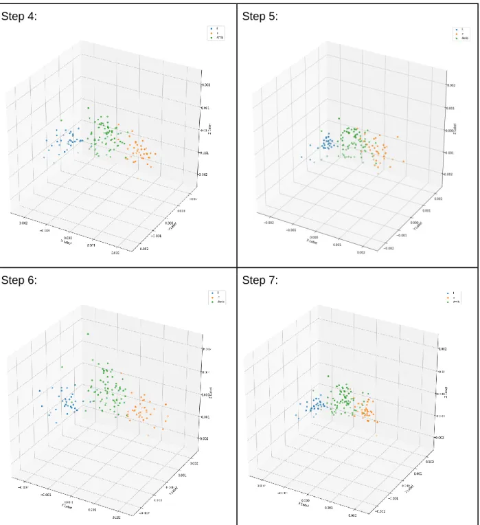
![Table 1. Visualization for the time-course of adaptation for the Baseline DNN model (green for ambiguous [l/r], orange for /r/ and blue for /l/)](https://thumb-us.123doks.com/thumbv2/123dok_us/1985534.2794877/46.918.110.817.164.949/table-visualization-course-adaptation-baseline-model-ambiguous-orange.webp)
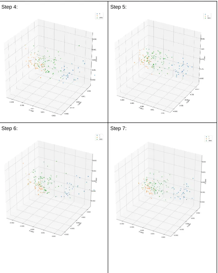
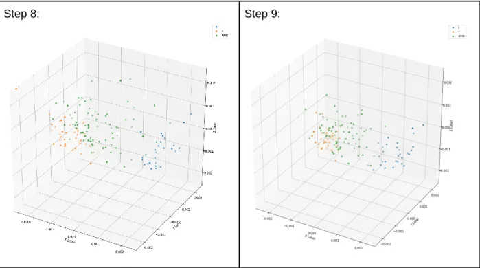
![Table 2. Visualization for the time-course of adaptation for the AmbL DNN model (green for ambiguous [l/r], orange for /r/ and blue for /l/)](https://thumb-us.123doks.com/thumbv2/123dok_us/1985534.2794877/49.918.116.814.203.984/table-visualization-course-adaptation-ambl-model-ambiguous-orange.webp)