Correlated Data with Missing Values
by Wei Ding
A dissertation submitted in partial fulfillment of the requirements for the degree of
Doctor of Philosophy (Biostatistics)
in The University of Michigan 2015
Doctoral Committee:
Professor Peter X-K Song, Chair Assistant Professor Veronica Berrocal Assistant Professor Hui Jiang
It was the best of time. It was the worst of time. For Charles Dickinson, it was French Revolution, but for me, it was my life in the past five years as a phd student in Ann Arbor. When I first came here, I was with curiosity, with fear, with doubt, and with uncertainty. I wish I can leave here with confidence, with independence, and with hope, to a bright future.
First and foremost, I am deeply grateful to my wonderful advisor, Dr. Peter Song, who encouraged me, inspired me, and helped me with great tolerance and patience. Without him, this dissertation is never made possible. I was moved by his rigorous thinking, broad vision, and his passion to statistics. Moreover, Dr. Peter Song is not just an advisor, but also a mentor, and a role model. I learned a lot from his thoughtfulness and kindness.
My thanks go out to Dr. Veronica Berrocal, Dr. Hui Jiang, and Dr. Qiaozhu Mei for serving on my dissertation committee and providing valuable suggestions and support on my research.
I am thankful for all my best friends in Ann Arbor and elsewhere around the world. With them, I had a great time, and never felt lonely.
The most important of all, I must thank my parents, who love me unconditionally, support me no matter what, and always have absolute faith in me. This thesis is dedicated to my beloved parents.
DEDICATION . . . ii
ACKNOWLEDGEMENTS . . . iii
LIST OF FIGURES . . . vi
LIST OF TABLES . . . vii
ABSTRACT . . . ix CHAPTER I. Introduction . . . 1 1.1 Summary . . . 1 1.2 Objectives . . . 3 1.3 Literature Review . . . 6 1.3.1 Correlated Data . . . 6 1.3.2 Missing Data . . . 7 1.3.3 Copula . . . 8 1.3.4 EM Algorithm . . . 9
1.3.5 Composite Likelihood Method . . . 10
1.3.6 Partial Identification . . . 10
1.3.7 Multilevel Model . . . 11
1.3.8 Motivating data I: Quality of Life Study . . . 11
1.3.9 Motivating data II: Infants’ Visual Recognition Memory Study . . 12
1.4 Outline of Dissertation . . . 13
II. EM Algorithm in Gaussian Copula with Missing Data . . . 14
2.1 Summary . . . 14
2.2 Introduction . . . 15
2.3 Model . . . 18
2.3.1 Location-Scale Family Distribution Marginal Model . . . 18
2.3.2 Gaussian Copula . . . 19
2.3.3 Examples of Marginal Models . . . 20
2.4 EM Algorithm . . . 21
2.4.1 Expectation and Maximization . . . 21
2.4.2 Examples Revisited . . . 26
2.4.3 Standard Error Calculation . . . 27
2.4.4 Initialization . . . 28
2.5 Simulation Study . . . 28
2.5.1 Skewed Marginal Model . . . 29
2.5.2 Misaligned Missing Data . . . 31
III. Composite Likelihood Approach in Gaussian Copula Regression Models
with Missing Data . . . 39
3.1 Summary . . . 39
3.2 Introduction . . . 40
3.3 Method . . . 45
3.3.1 Complete-Case Composite Likelihood . . . 45
3.3.2 Likelihood Orthogonality . . . 46
3.3.3 Large-Sample Properties . . . 49
3.3.4 Estimation of Partially Identifiable Parameters . . . 50
3.4 Implementation . . . 53
3.5 Gaussian Copula Regression Model . . . 54
3.5.1 Location-Scale Family Distribution Marginal Model . . . 54
3.5.2 Gaussian Copula . . . 55
3.5.3 Complete-Case Composite Likelihood . . . 56
3.5.4 Implementation . . . 57
3.6 Simulation Experiments . . . 58
3.6.1 Three-Dimensional Linear Regression Model . . . 58
3.6.2 Integration of Four Data Sources . . . 61
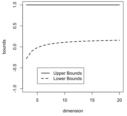
3.6.3 Estimation with Two Partially Identifiable Parameters . . . 62
3.7 PROMIS Data Analysis . . . 65
3.8 Concluding Remarks . . . 66
IV. Multilevel Gaussian Copula Regression Model . . . 72
4.1 Summary . . . 72
4.2 Introduction . . . 73
4.3 EEG Data . . . 74
4.3.1 Data Exploration . . . 76
4.3.2 Mixed Effects Model . . . 77
4.4 Model . . . 84
4.4.1 Location-scale Family Marginal Model . . . 85
4.4.2 Gaussian Copula . . . 85
4.4.3 Example of Marginal Model: Gamma Margin . . . 87
4.5 Maximum Likelihood Estimation . . . 87
4.5.1 Log Likelihood Function . . . 88
4.5.2 Peeling Algorithm . . . 88
4.5.3 Statistical Inference . . . 90
4.6 Simulation Study . . . 90
4.6.1 Multilevel Model with Normal Margins I . . . 91
4.6.2 Multilevel Model with Normal Margins II . . . 92
4.7 Analysis of EEG Data . . . 94
4.8 Conclusions & Discussion . . . 97
V. Discussions and Future Works . . . 100
APPENDIX . . . 102
BIBLIOGRAPHY. . . 108
Figure
1.1 Connection and Structure of the Dissertation . . . 13 2.1 Plots of observed and predicted residuals from the EM algorithm. . . 35 3.1 Upper and Lower Bounds for a Partially Identifiable Correlation Parameter . . . . 52 3.2 Bounds for Partial Identifiable Parameters . . . 64 4.1 Contour of the 128-Channel EEG Sensor Net (L: left; R: right; A: anterior; P:
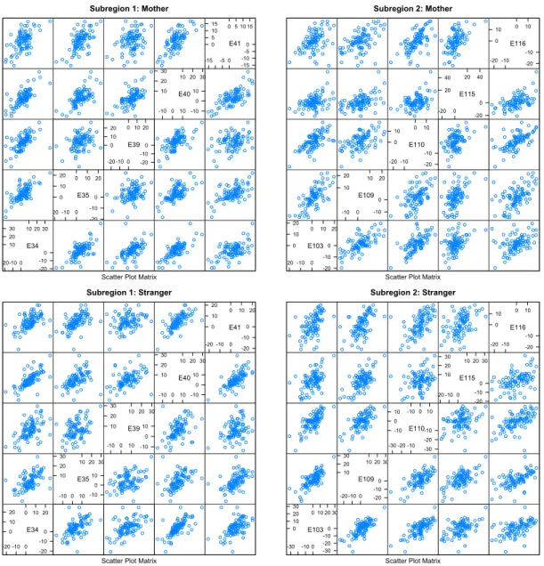
posterior) . . . 75 4.2 LSW related time series cross-classified by iron status and stimulus. . . 76 4.3 Density of LSW measurements at each electrodes over stimulus level. . . 78 4.4 Scatter Plot of LSW Measurements in Each Subregion Stratified by Pictorial
Stim-uli. . . 80 4.5 Scatter Plot of LSW Measurements in Each Subregion Stratified by Pictorial
Stim-uli. . . 81 4.6 Boxplots of region-specific LSW cross iron status and stimulus. . . 82 4.7 Boxplots of region-specific LSW cross iron status and stimulus. . . 83 4.8 Z-statistics of Iron Status Effect on Mother’s and Stranger’s Pictorial Stimuli . . . 98
Table
2.1 Simulation results of correlation (Kendall’s tau) parameters estimation in copula model for marginal skewed distributed data obtained by full data likelihood, EM algorithm and Imputation methods with different missing percentage. (Standard error ratio is calculated by a ratio of two standard errors between a method and the gold standard.) . . . 30 2.2 Simulation results concerning estimation of Pearson correlation and marginal
re-gression parameters in the copula model for partially misaligned missing at random data obtained EM algorithm, compared with the gold standard with full data, Mul-tiple Imputation and Hot-Deck Imputation. (Standard error ratio is calculated by a ratio of two standard errors between a method and the gold standard.) . . . 33 2.3 Estimation of correlation and marginal regression parameters in the copula model
for quality of life study obtained by univariate analysis, EM algorithm and Multiple Imputation. . . 35 3.1 Summary of simulation results, including average point estimates, empirical
stan-dard errors (ESE) and average model-based stanstan-dard errors (AMSE), under the misaligned missing data pattern for 3-dimensional linear regression model. . . 68 3.2 Summary of simulation results in the integration of four data sets, including average
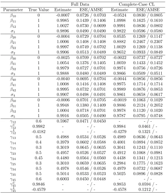
point estimates, empirical standard errors (ESE) and average model-based standard errors (AMSE), under various missing data patterns over four different data sources, each of which is generated from a three-dimensional linear regression model . . . . 69 3.3 Summary of simulation results in a 5-dimensional linear model, including average
point estimates, empirical standard errors (ESE) and average model-based standard errors (AMSE), under two pairs of misaligned missingness between the first and second margins and between the fourth and fifth margins, respectively. . . 70 3.4 Estimation of correlation and marginal regression parameters for quality of life
study obtained by complete-case univariate analysis, EM algorithm with two initial values of correlation parameters, two runs multiple imputations, and one method of complete-case composite likelihood. . . 71 4.1 Summary of Pearson Correlation of LSW Measurements in Each Subregion
Strati-fied by Pictorial Stimuli . . . 79 4.2 Maximum Likelihood Estimates of the Fixed Effects . . . 84 4.3 Restricted Maximum Likelihood Estimates of the Variance Components . . . 84
level Gaussian copula regression model is compared with the univariate analysis, including average point estimates, empirical standard errors (ESE) and average model-based standard errors (AMSE) over 1000 running of simulations. . . 93 4.5 Summary of simulation results in four-level correlated normally distributed margins
with Mat´ern correlation, exchangeable correlation, AR-1 correlation, and unstruc-tured correlation obtained from the multilevel Gaussian copula regression model, including average point estimates and empirical standard errors (ESE). . . 94 4.6 Summary of iron status effect on LSW measurements collected from each node and
each stimulus, including estimate, model-based standard errors, and z-statistics. . . 96 4.7 Summary of estimation results for the correlation parameters. . . 97
Copula Regression Models for the Analysis of Correlated Data with Missing Values by
Wei Ding
Advisor: Peter X-K Song
The class of Gaussian copula regression models provides a unified modeling frame-work to accommodate various marginal distributions and flexible dependence struc-tures. In the presence of missing data, the Expectation-Maximization (EM) algo-rithm plays a central role in parameter estimation. This classical method is greatly challenged by multilevel correlation, a large dimension of model parameters, and a misaligned missing data mechanism encountered in the analysis of data from col-laborative projects. This dissertation will develop a series of new methodologies to enhance the effectiveness of the EM algorithm in dealing with complex correlated data analysis via a combination of new concepts, estimation approaches, and com-puting procedures. The dissertation consists of three major projects given as follows. The focus of Project 1 is on the development of an effective EM algorithm in Gaussian copula regression models with missing values, in which univariate location-scale family distributions are utilized for marginal regression models and Gaussian copula for dependence. The proposed class of regression models includes the classical multivariate normal model as a special case and allows both Pearson correlation and rank-based correlations (e.g. Kendall’s tau and Spearman’s rho). To improve the
an effective peeling procedure in the M-step to sequentially maximize the observed log-likelihood with respect to regression parameters and dependence parameters. In addition, the Louis formula is provided for the calculation of the Fisher information. The EM algorithm is tailored for misaligned missing data mechanism under struc-tured correlation structures (e.g. exchangeable and first-order autoregression). We run simulation studies to evaluate the proposed model and algorithm, and to compare with both model-based multiple imputation and hot-deck imputation methods.
Project 2 is devoted to a critical extension of Project 1, where the assumption of structured correlation structure is relaxed, so the resulting model and algorithm can be applied to deal with complex correlated data with missing values. The key new contribution in the extension concerns the development of EM algorithm for composite likelihood estimation in the presence of misaligned missing data. We pro-pose the complete-case composite likelihood, which is more general than the classical pairwise composite likelihood, to handle both point-identifiable and partially identi-fiable parameters in the Gaussian copula regression model. Estimation of a partially identifiable correlation parameter is given by an estimated interval. Both estima-tion properties and algorithmic convergences are discussed. The proposed method is evaluated and illustrated by simulation studies and a quality-of-life data set.
Motivated by an electroencephalography (EEG) data collected from 128 electrodes on the scalps of 9 months old infants, Project 3 concerns the regression analysis of multilevel correlated data. Indeed multilevel correlated data are pervasive in practice, which is routinely modeled by the hierarchical modeling system using random effects. We develop an alternative class of parametric regression models using Gaussian cop-ulas and implement the maximum likelihood estimation. The proposed model is very
discrete outcomes or outcomes of mixed types; and in the aspect of dependence, it can allow temporal (e.g. AR), spatial (e.g. Matern), clustered (e.g. exchangeable), or combined dependence structures. Parameters in the proposed model have marginal interpretation, which is absent in the hierarchical model when outcomes of interest are non-normal (e.g. binary or ordinal categorical). Moreover, it allows the presence of missing data. The proposed EM algorithm with peeling procedure provides a fast and stable parameter estimation algorithm. The proposed model and algorithm are assessed by simulation studies, and further illustrated by the analysis of EEG data for the adverse effect of iron deficiency on infants’ visual recognition memory.
Introduction
1.1 Summary
The class of Gaussian copula regression models provides a unified modeling frame-work to accommodate various marginal distributions and flexible dependence struc-tures. In the presence of missing data, the Expectation-Maximization (EM) algo-rithm plays a central role in parameter estimation. This seminal method is greatly challenged by complex data structures, such as multilevel correlation, large dimension of model parameters, and a misaligned missing data pattern that we have encoun-tered in our collaborative projects at University of Michigan. This dissertation aims to develop a set of new statistical methodologies and algorithms to enhance the ap-plications of the EM algorithm to deal with complex correlated data analysis. Based on new concepts, estimation approaches, and computing procedures as well as their combinations, we hope to yield more flexible and effective analytic tools to analyze complex correlated data. The dissertation consists of three major projects described as follows.
Project 1 focus on the development of an effective EM algorithm in Gaussian cop-ula regression models with missing values, in which univariate location-scale family distributions are utilized for marginal regression models and Gaussian copula for
dependence. The proposed class of regression models includes the classical mul-tivariate normal model as a special case and allows both Pearson correlation and rank-based correlations (e.g. Kendall’s tau and Spearman’s rho). To improve the implementation of the EM algorithm, following Meng and Rubin (1993), we establish an effective peeling procedure in the M-step to sequentially maximize the observed log-likelihood with respect to regression parameters and dependence parameters. In addition, Louis’ formula is provided for the calculation of the Fisher information. The EM algorithm is particularly tailored for the so-called misaligned missing data mechanism under structured correlation structures (e.g. exchangeable and first-order autoregression). We run extensive simulation studies to evaluate the proposed model and algorithm, and to compare our method with both model-based multiple impu-tation and hot-deck impuimpu-tation methods.
Project 2 is devoted to a critical extension of Project 1, where the assumption of structured correlation structure is relaxed, so the resulting model and algorithm can be applied to deal with complex correlated data with missing values. The key new contribution in the extension concerns the development of the peeling algorithm for composite likelihood estimation in the presence of misaligned missing data pattern. We propose the complete-case composite likelihood for estimation, which is more general than the classical pairwise composite likelihood. The proposed method is in-tended to handle both point-identifiable and partially identifiable parameters in the Gaussian copula regression model. Estimation of a partially identifiable correlation parameter is given by an estimated interval. Both estimation properties and algorith-mic convergences are discussed. The proposed method is evaluated and illustrated by simulation studies and a quality-of-life data set.
on the scalps of 9 months old infants, Project 3 concerns the regression analysis of multilevel correlated data. Arguably, multilevel correlated data are pervasive in practice, which is routinely modeled by the hierarchical modeling system using ran-dom effects. We develop an alternative class of parametric regression models using Gaussian copulas and implement the maximum likelihood estimation. The proposed model is very flexible; in the aspect of regression model, it can accommodate contin-uous outcomes, discrete outcomes or outcomes of mixed types; and in the aspect of
dependence, it can allow temporal (e.g. AR), spatial (e.g. Mat´ern), clustered (e.g.
exchangeable), or a mixture of dependence structures. Parameters in the proposed model have marginal interpretation, which is absent in the hierarchical model when outcomes of interest are non-normal (e.g. binary or ordinal categorical). Moreover, it allows the presence of missing data. The proposed EM algorithm with peeling procedure provides a fast and stable iterative procedure for parameter estimation algorithm. The proposed model and algorithm are assessed by simulation studies, and further illustrated by the analysis of EEG data for the adverse effect of iron deficiency on infant’s visual recognition memory.
1.2 Objectives
The Objective of Chapter II is to develop the Gaussian copula regression model (Song (2000); Song et al. (2009a)) to analyze correlated data with missing values. The proposed class of multidimensional regression models for correlated data have various meritorious features that have led to its popularity in practical studies. First, the copula regression model allows to define, evaluate and interpret correlations between variables in a full probability manner, in a very similar way to that of the classical multivariate normal distribution which has been extensively studied in the statistical
literature and widely applied in the analysis of multivariate data. Second, from the copula regression model various types of correlations are furnished to address differ-ent questions related to a joint regression analysis. For example, depending on if the marginal distributions are normal or skewed, it provides Pearson linear correlation or rank-based nonlinear correlations (e.g., Kendall’s tau or Spearman’s rho). Moreover, these correlations types may be represented either in a form of unconditional pair-wise correlation, or in a form of conditional pairpair-wise correlation. Third, the copula regression model has the flexibility to incorporate marginal location-scale families to adjust for confounding factors, which is of practical importance. Last, the availabil-ity of the full joint probabilavailabil-ity model gives rise to the great ease of implementing powerful EM algorithm to handle missing data in a broad range of multi-dimensional models where the regression parameters in the mean model and the correlation pa-rameters can be estimated simultaneously under one objective function. In such a framework, both estimation and inference are safeguarded by the well-established classical maximum likelihood theory.
Largely motivated by a collaborative project concerns a quality of life study on children with nephrotic syndrome, the objective of Chapter III centers on a further extension of the Gaussian copula regression analysis methodology proposed in Chap-ter II by addressing two challenging problems. One is the difficulty of estimating correlation parameters when misaligned missing pattern occurs between variables. By misaligned missingness we mean a missing data pattern in which two variables are measured in disjoint subsets of subjects and have no overlapped observations. The other is the issue of parameter identifiability, which is a serious consequence from misaligned missing data pattern encountered in the estimation of unstructured correlation matrix. Note that estimating correlation matrix is indeed required in a
joint regression analysis of multiple correlated outcomes. We propose a complete-case composite likelihood method to perform estimation and inference for the model parameters, in which the above two major methodological challenges are handled via a composition of are marginal distributions of observed variables. Also, the cor-relation parameters that are not point-identified are estimated by both lower and upper bounds that form interval estimation for the partially identifiable parameters. For implementation, the effective peeling optimization procedure is modified for the composite likelihood to estimate point-identifiable parameters. We investigate the performance of complete case composite likelihood method, and compare it with the maximum likelihood estimation given in Chapter II through simulation studies.
The objective of Chapter IV focuses on the development of Gaussian regression models for multilevel correlated data. This work is motivated by a collaborative project that aims to assess the adverse effect of prenatal iron deficiency on infant’s visual recognition memory. In this study, memory is measured by electroencephalog-raphy (EEG) sensor net of 128 electrodes, from which event-related potential (ERP) such as low slow wave is extracted to quantify the capacity of memory. A major technical challenge arises from a multilevel dependence structure, including tempo-ral, spatial and clustered correlations. When an ERP outcome is skewed, multilevel rank-based correlations are appealing, which are naturally supplied by the Gaussian copula model. Thus, in this project we extend the framework of Gaussian copula regression models by accommodating multiple types of correlations. This flexibility of dependence modeling allows us to analyze complex data structures in the regres-sion analysis and to provide more comprehensive results than those obtained by a subset of data with one-level correlation. This extension of copula model to mul-tilevel correlation is established by the utility of Kronecker product of correlation
matrices. We also extend the peeling procedure to carry out estimation of the model parameters, which is particularly useful to deal with potentially a large number of correlation parameters. Both simulation studies and data analysis examples will be provided to illustrate the proposed methodology. In the presence of missing data, the EM algorithm with the peeling procedure is used in implementation.
1.3 Literature Review
The amount of the literature related to my dissertation research topics is so vast that it is not possible to review all major articles in this chapter. Instead, below I attempt to provide my review based on the set of references that I have actually read in a reasonable detail.
1.3.1 Correlated Data
Multi-dimensional regression models for correlated data involve typically the spec-ification of both correlation structures and marginal mean models that can be formu-lated by the classical univariate generalized linear model (GLM) (Nelder and Baker (1972)). Although the great popularity of quasi-likelihood approaches to analyzing correlated data, such as generalized estimating equation (GEE) (Liang and Zeger (1986)) and quadratic inference function (QIF) (Qu et al. (2000)), a fully specified probability model with interpretable correlation structures is actually a desirable formulation to address the need of evaluating correlations between variables. It is known that in the quasi-likelihood method correlations are treated as nuisance pa-rameters, so that their estimation and interpretation are not of primary interest in data analysis. This treatment may not always be desirable and can be improved by some will-behaved dependence models such as copula models (Joe (1997)).
1.3.2 Missing Data
Missing data is an important issue in statistics, and can deliver a significant influence on the conclusions. There are many reasons for the occurrence of missing data: no information is collected for some subjects, certain subjects are unwilling to provide sensitive or private information, subject’s dropout due to moving, or researcher cannot collect the whole data due to time or budgetary limitations.Three mechanisms of missing data (Rubin, 1976, Rubin (1976)) are commonly considered in the data analysis, including (i) missing completely at random (MCAR) when the missing mechanism is independent from both observed and missing data; (ii) missing at random (MAR) when the missing mechanism is not related to missing data; and (iii) missing not at random (MNAR) when the missing mechanism depends on missing.
In terms of handling missing data, the complete case analysis, which is often used in practice for convenience, simply discards any cases with missing values on those of the variables selected and proceeds with the analysis using standard methods. Obviously, the data attrition reduces the sample size, resulting potentially in a great loss of estimation efficiency. EM algorithm (Dempster et al. (1977)) is a widely used iterative algorithm to carry out the maximum likelihood estimation in a sta-tistical analysis with incomplete data. Multiple Imputation (Rubin (2004)) provides an alternative approach useful to deal with statistical analysis with missing values. Instead of filling in a single value for each missing value, (Rubin (2004)) multiple imputation procedure actually replaces each missing value with a set of plausible values that represent the uncertainty about the right value to impute. When data come from skewed distributions, hot-deck Imputation (Andridge and Little (2010)) is also widely used, where a missing value is imputed with a randomly drawn similar
record in terms of the nearest neighbors criterion. One caveat of hot-deck imputa-tion is that it is a single imputaimputa-tion method, which may fail to provide desirable uncertainty associated with missing values. In addition, the number of imputed data sets is critical to obtain proper data analysis results, and a small number may lead to inappropriate inference. Some researchers have recommended 20 to 100 imputa-tion data sets or even more (Graham et al. (2007)), which appears computaimputa-tionally costly in practice. The imputation methods may become nontrivial and no longer straightforward when data distributions are skewed and adjusting for confounding factors is needed.
1.3.3 Copula
Copula is a joint multivariate probability distribution of random variables, and the marginal probability distribution of each variable is uniform, and is used to model the dependence between random variables. Sklar’s Theorem (Sklar (1959)) states that for a multivariate joint distribution, there exists a suitable copula that not only links the univariate marginal distribution functions, but also captures the dependence. The representation of a copula model separates the marginal models and the dependence model.
Most of recently published works on the copula regression models have been fo-cused on analyzing fully observed data; for example, Song (2007); Czado (2010); Joe et al. (2010); Genest et al. (2011); Masarotto et al. (2012); Acar et al. (2012). There is little knowledge available concerning how the analysis may be done in the presence of missing data.
Gaussian copula is a generated model from multivariate normal distribution by inverse normal transformation, where the correlation matrix under Gaussian copula is the Pearson correlation matrix of the normal distributed quantiles. Gaussian
cop-ula regression model (Song (2000); Song et al. (2009a)) is an useful probability model for the correlated data because of the following meritorious features. First, the Gaus-sian copula regression model allows us to define, evaluate and interpret correlations between variables in a full probability manner, and the classical multivariate normal distribution is a special the Gaussian copula regression model. Second, from the cop-ula model various types of correlations are provided to answer for different questions. For example, it provides Pearson linear correlation or rank-based nonlinear correla-tions (Kendall’s tau or Spearman’s rho), depending on if the marginal distribucorrela-tions are normal or skewed. Moreover these correlations may be obtained either in a form of unconditional marginal pairwise correlation, or in a form of conditional pair-wise correlation. Third, the copula model has the flexibility to incorporate marginal GLMs to adjust for confounding factors, which is of practical importance. Last, the availability of the full probability model gives rise to the great ease of implementing powerful EM algorithm to handle missing data in a broad range of multi-dimensional models where the regression parameters in the mean model and the correlation pa-rameters can be estimated simultaneously under one objective function. In such a framework, both estimation and inference are safeguarded by the well-established classical maximum likelihood theory.
1.3.4 EM Algorithm
The EM algorithm proposed by Dempster et al. (1977) is widely used to find the maximum likelihood estimators of a statistical model in cases where the equations cannot be solved directly, or with the presence of missing data. It contains two it-erative steps. Expectation step (E-step) calculates the expectation of the observed log likelihood function, based on the conditional distribution of missing data given observed data under estimate of the parameters of current iteration, and
maximiza-tion step (M-step) finds the parameter that maximize the observed log likelihood function.
In the expectation conditional maximization (ECM) algorithm proposed by Meng and Rubin (1993), each M-step is replaced with a sequence of conditional maximiza-tion steps (CM-steps) where one or a group of parameters are maximized sequentially, conditionally on the other parameters being fixed.
1.3.5 Composite Likelihood Method
Composite likelihood (Lindsay (1988)) has received increasing attention in the recent statistical literature. It is also known as a pseudo likelihood (Molenberghs and Verbeke (2005)) in longitudinal data setting, or an approximate likelihood (Stein et al. (2004)) in spatial data setting, or a quaisi-likelihood (Hjort et al. (1994); Glasbey (2001); Hjort and Varin (2008)) in spatial and time series data settings.
As composite likelihood may be treated as a special class of inference functions, statistical inference can be established by an application of the standard theory of inference functions (Chapter 3, Song (2007)). For example, Godambe information matrix (Godambe (1960)) is typically used to obtain the asymptotic variance of a composite likelihood estimator, and in the presence of missing data, Godambe information matrix is calculated according to an empirical procedure suggested by Gao and Song (2011).
1.3.6 Partial Identification
For the case of completely misaligned missingness considered in this thesis, for the unstructured correlation matrix, some of correlation parameters may not be fully identifiable. Manski (2003) proposed several approaches to address such a partial identification problem in parameter estimation. A parameter is said to be partially
identifiable if the true parameter is not point-identifiable but a range of parame-ter values containing the true value is identifiable. Fan and Zhu (2009) provided a method to determine the lower and upper bounds of the parameter range in the set-ting of bivariate copula models, where the pairwise correlation parameter is partially identified by an estimated parameter range. However, Fan and Zhu (2009)’s method
does not work for a general d-dimensional copula model, and it is not clear at this
moment how easily an extension of their method may be accomplished analytically. This thesis aims to develop a new composite likelihood method to overcome this estimation difficulty.
1.3.7 Multilevel Model
Multilevel data, also known as hierarchical data, clustered data, and nested data, are a common type of data structure in spatio-temporal analysis, or when subjects are grouped by some specific clusters. For example, Aitkin and Longford (1986) designed a two-level model for educational data, in which students are clustered in schools. Random effects model, also known as variance components model, is one of the most popular methods to estimate parameters in multilevel models.
Random effects model was introduced by Laird and Ware (1982), where both “fixed” and “random” effects are respectively referred to as the population-average and subject-specific effects. Related theories and applications of random effects mod-els in data analysis may be found in Verbeke et al. (2010); Liang and Zeger (1986); Zeger et al. (1988), and Zeger and Liang (1986), among others.
1.3.8 Motivating data I: Quality of Life Study
Nephrotic Syndrome (NS) is a common disease in pediatric patients with kidney disease. The typical symptom of this disease is characterized by the presence of
edema that significantly affects the health-related quality of life in children and ado-lescents. The PROMIS (Fries et al. (2005); Gipson et al. (2013)) is a well-validated instrument to assess pediatric patient’s quality of life. The instrument consists of 7 domains, including pain interference, fatigue, depression, anxiety, mobility, social peer relationship, and upper extremity functioning. In the data, two QoL scores, pain and fatigue, are measured on two exclusive sets of subjects due to some logistic difficulty at the clinic. That is, out of 224 subjects, 107 subjects have QoL measure-ments of pain, but no QoL measuremeasure-ments of fatigue, while the other 117 subjects have QoL measurements of fatigue but no QoL measurements of pain. Interestingly, QoL measurements of anxiety have been fully recorded on all 224 individuals with no missing data.
1.3.9 Motivating data II: Infants’ Visual Recognition Memory Study
Infants’ visual recognition memory study aims to evaluate whether or not, and if so, how, iron deficiency affects visual recognition memory for infants. We refer to some of important related work that has been summarized in de Haan et al. (2003). Infants’ memory capability is measured by the activity of the brain during a period of 1700 milliseconds using electroencephalograph (EEG) net with 128-channel sensors on the scalp (Reynolds et al. (2011)). The data collection occurs at two time points: when an infant sees his/her mother’s picture and when he or she sees a stranger’s picture. At each time point, an event-related potential (ERP) of interest, late slow wave (LSW), is extracted from after the standard data processing, which is widely used as primary outcomes of visual recognition memory. In total, there are 91 children in this study, with fully observed data. 20 out of 128 electrodes are of interest with 5 in each of the four subregions.
1.4 Outline of Dissertation
This dissertation is organized as follows: In Chapter I, we give an overview about my dissertation and an introduction to related works. In Chapter II, we develop a peeling algorithm in Gaussian copula regression model and provide a solution to the misaligned missing data pattern. In Chapter III, we present a complete-case compos-ite likelihood method as an alternative solution to the analysis of missing data with the misaligned missing pattern, which Gaussian copula regression model is used as an example to illustrate this approach. In Chapter IV, a multilevel Gaussian copula regression model is developed with peeling algorithm. In concluding some discussions and future work are presented in Chapter V. The connection and structure between Chapter II, III, are IV are displayed in Figure 1.1.
Figure 1.1: Connection and Structure of the Dissertation
Chapter 2
Chapter 3
Chapter 4
MLE Composite Likelihood
(Misaligned ) Missing Data Multilevel Data Structure EM
Algorithm Algorithm Peeling
Gaussian Copula Regression Method: Model: Data Structure: Chapter: Algorithm:
EM Algorithm in Gaussian Copula with Missing Data
2.1 Summary
Rank-based correlation is widely used to measure dependence between variables
when their marginal distributions are skewed. Estimation of such correlation is
challenged by both the presence of missing data and the need for adjusting for con-founding factors. In this paper, we consider a unified framework of Gaussian copula regression that enables us to estimate either Pearson correlation or rank-based cor-relation (e.g. Kendall’s tau or Spearman’s rho), depending on the types of marginal distributions. To adjust for confounding covariates, we utilize marginal regression models with univariate location-scale family distributions. We establish the EM al-gorithm for estimation of both correlation and regression parameters with missing values. For implementation, we propose an effective peeling procedure to carry out iterations required by the EM algorithm. We compare the performance of the EM algorithm method to the traditional multiple imputation approach through simula-tion studies. For structured types of correlasimula-tions, such as exchangeable or first-order auto-regressive (AR-1) correlation, the EM algorithm outperforms the multiple im-putation approach in terms of both estimation bias and efficiency.
2.2 Introduction
Estimation of rank-based correlation is frequently required in practice to evaluate relationships between variables when they follow marginally skewed distributions. However, estimation of such correlation becomes a great challenge in the presence of missing data and with the need of adjusting for confounders. Most of recently published works on the copula models have been focused on analyzing fully observed data, e.g., Czado (2010); Joe et al. (2010); Genest et al. (2011); Masarotto et al. (2012); Acar et al. (2012), and there is little knowledge available concerning how the analysis may be done in the presence of missing data.
In terms of handling missing data, the complete case analysis, which is often used in practice for convenience, simply discards any cases with missing values on those of the variables selected and proceeds with the analysis using standard methods. Obviously, the data attrition reduces the sample size, resulting potentially in a great loss of estimation efficiency. EM algorithm (Dempster et al. (1977)) is a widely used iterative algorithm to carry out the maximum likelihood estimation in a sta-tistical analysis with incomplete data. Multiple Imputation (Rubin (2004)) provides an alternative approach useful to deal with statistical analysis with missing values. Instead of filling in a single value for each missing value, (Rubin (2004)) multiple imputation procedure actually replaces each missing value with a set of plausible values that represent the uncertainty about the right value to impute. When data come from skewed distributions, Hot-Deck Imputation (Andridge and Little (2010)) is also widely used, where a missing value is imputed with a randomly drawn similar record in terms of the nearest neighbor criterion. One caveat of Hot-Deck imputa-tion is that it is a single imputaimputa-tion method, which may fail to provide desirable
uncertainty associated with missing values. In addition, the number of imputed data sets is critical to obtain proper data analysis results, and a small number may lead to inappropriate inference. Some researchers have recommended 20 to 100 imputa-tion data sets or even more (Graham et al. (2007)), which appears computaimputa-tionally costly in practice. The imputation methods may become nontrivial and no longer straightforward when data distributions are skewed and adjusting for confounding factors is needed.
Multi-dimensional regression models for correlated data involve typically the spec-ification of both correlation structures and marginal mean models that can be formu-lated by the classical univariate generalized linear model (GLM) (Nelder and Baker (1972)). Although the great popularity of quasi-likelihood approaches to analyzing correlated data, such as generalized estimating equation (GEE) (Liang and Zeger (1986)) and quadratic inference function (QIF) (Qu et al. (2000)), a fully specified probability model with interpretable correlation structures is actually a desirable device to achieve the objective of evaluating correlations between variables. It is known that in the quasi-likelihood method correlations are treated as nuisance pa-rameters, so that their estimation and interpretation are not of primary interest in data analysis.
In this paper we consider the Gaussian copula regression model (Song (2000); Song et al. (2009a)) as the probability model for the correlated data because of the following meritorious features. First, the copula model allows us to define, evaluate and interpret correlations between variables in a full probability manner, very similar to the classical multivariate normal distribution. Second, from the copula model var-ious types of correlations are provided to answer for different questions. For example, it provides Pearson linear correlation or rank-based nonlinear correlations (Kendall’s
tau or Spearman’s rho), depending on if the marginal distributions are normal or skewed. Moreover these correlations may be obtained either in a form of uncondi-tional marginal pairwise correlation, or in a form of condiuncondi-tional pairwise correlation. Third, the copula model has the flexibility to incorporate marginal GLMs to adjust for confounding factors, which is of practical importance. Last, the availability of the full probability model gives rise to the great ease of implementing powerful EM algorithm to handle missing data in a broad range of multi-dimensional models where the regression parameters in the mean model and the correlation parameters can be estimated simultaneously under one objective function. In such a framework, both estimation and inference are safeguarded by the well-established classical maximum likelihood theory.
It is of interest in the context of copula models to investigate and compare the two principled methods of handling missing data, EM algorithm and multiple im-putation, as well as their computational complexity. Since the development of the EM algorithm is not trivial in the framework of Gaussian copula models, we propose an efficient peeling procedure to update model parameters in the M-step due to the involvement of a multi-dimensional integral. To adjust for confounding factors in the marginals, we focus on the location-scale family distribution in marginal regression models to embrace the flexibility of marginal distributions.
We compare the performance of the EM algorithm to the multiple imputation approach through simulation studies. For structured types of correlations, such as exchangeable or first-order auto-regressive (AR-1) correlation matrix, the EM al-gorithm method outperforms the multiple imputation approach in both aspects of estimation bias and efficiency. These two approaches perform similarly when the correlation matrix is unstructured.
This paper is organized as follows. Section 2.3 describes the Gaussian cop-ula model. Together with some examples of practically useful models, Section 2.4 presents the details of the EM algorithm and Louis’ formula (Louis (1982)) for stan-dard error calculation. Section 2.5 presents simulation study, and a data analysis is included in Section 2.6. Section 2.7 provides some concluding remarks.
2.3 Model
The focus of this paper is on using EM algorithm in Gaussian copula to estimate
of correlation with missing data. We assume that there are n partially observed
subjects. For a subject, let Y = (y1, y2,· · ·, yd)0 be a d-dimensional random vector
of continuous outcomes, part of which is observed and the other part is missing.
Denote by Rj as a missing data indicator, where Rj = 0 or 1 if the jth element yj
is missing or observed. Note that this indicator is known but varies for different
subjects. Let ymis be the set of variables with missing data, and yobs be the set of
variables with observed data of a subject.
2.3.1 Location-Scale Family Distribution Marginal Model
Suppose θ = (θ1, θ2,· · · , θd)0, where each θj denotes a set of marginal parameters
associated with thejth(j = 1,· · · , d) marginal density function,f
j(yj|θj). Denote by
uj = Fj(yj|θj) the marginal cumulative distribution function(CDF) corresponding
to the jth margin, where F
j is a location-scale family distribution parametrized by
a location parameter µj and a positive scale parameter σj, θj = (µj, σj). More
specifically, the marginal location-scale density function is given by
(2.1) fj(yj|θj) = 1 σj ˜ f yj −µj σj , j = 1,· · · , d,
where ˜f(·) is the standard kernel density withRRyf˜(y)dy= 0, andRRy2f˜(y)dy= 1.
and parameter µj orσj may be modelled as a function of confounding covariates.
2.3.2 Gaussian Copula
A copula is a multivariate probability distribution in which the marginal
prob-ability distribution of each variable is uniform on (0,1). Sklar’s theorem (Sklar
(1959)) states that every multivariate cumulative distribution function of a continu-ous random vector Y = (y1, y2,· · · , yd)0 with marginals Fj(yj|θj) can be written as
F(y1, . . . , yd) = C(F1(y1), . . . , Fd(yd)), where C is a certain copula. In this paper,
Y is assumed to follow ad-dimensional distribution generated by a Gaussian copula
(Song (2000)), whose density function is given by
(2.2) f(Y|θ,Γ) =c(u|Γ)
d
Y
j=1
fj(yj|θj), u= (u1, u2,· · · , ud)0 ∈[0,1]d,
where c(u|Γ) = c(u1,· · · , ud|Γ), u ∈ [0,1]d, is the Gaussian copula density, with
uj =Fj(yj|θj),i= 1,· · · , d, and Γ is and×d matrix of correlation.
Let qj =qj(uj) = Φ−1(uj) be the jth marginal normal quantile, where Φ is CDF
of the standard normal distribution. According to Song (2007), the joint density of
a Gaussian copula functionc(·|Γ) takes the form:
(2.3) c(u|Γ) =|Γ|−12 exp 1 2Q(u) T(I−Γ−1)Q(u) , u∈[0,1]d
where Γ = [γj1j2]d×dis the Pearson correlation matrix ofQ(u) = (q1(u1),· · · , qd(ud)) 0,
and I is the d×d identity matrix. Here | · | denotes the determinant of a matrix.
Marginally, uj ∼ Uniform(0,1), and qj ∼ Normal(0,1). When yj is marginally
normal distributed, matrix Γ gives the Pearson correlation matrix ofY; otherwise, Γ
represents as a matrix of pairwise rank-based correlations. In fact, given a matrix Γ in
equation (4.3), two types of pairwise rank-based correlations, Kendall’s tau ([τj1j2]d×d
) and Spearman’s rho ([ρj1j2]d×d) can be obtained as follows: τj1j2 = 2
and ρj1j2 = 6
πarcsin(
γj1j2
2 ) for j1, j2 = 1,· · · , d, j1 6= j2, respectively (McNeil et al. (2010)).
2.3.3 Examples of Marginal Models
Among many possible marginal models, here we present two examples of marginal models to illustrate our proposed method, with or without the inclusion of covariates. These two following models are practically useful.
Example-1: Marginal Parametric Distribution
To adjust for confounding factors in the mean marginal model, let Xi = (1, xTi )T,
i = 1,· · · , n. For the jth margin, the linear model is imposed on the location
parameter in equation (3.11), µij = E(yij|Xi) = h(XiTβj), j = 1,· · · , d, where
βj = (βj0, βj1,· · · , βjp)0is a (p+1)-element unknown regression vector, andhis a link
function. For convenience, denote the resulting model by Yij ∼Fj(yj|µij(βj), σj).
As an important special case, we consider p = 0 (no covariates), and thus µij =
h(βj0) is a common parameter for all subjects i = 1,· · · , n. More generally, the
marginal distribution model with the CDF uij = Fj(yj|θj) may be a generalized
location-scale family distribution, such as gamma distribution, of which the loca-tion parameter is 0, and the estimaloca-tion procedure remains the same under a given marginal parametric distribution. This will be discussed as an example in simulation study in Section 2.5.1.
Example-2: Semi-parametric Marginal Distribution
If the type of the density function fj(yj), j = 1,· · · , d is unknown, there are
several possible forms available to specify equation (3.11). In this paper, we consider
estimated using the empirical distribution function. In this case, all the marginal
parameter θj is absorbed into the CDF.
2.4 EM Algorithm
Our goal is to estimate the model parameter (θ,Γ) in the presence of missing
data. This may be achieved by utilizing the EM algorithm. We propose an effective peeling procedure in the EM algorithm, which serves as a core engine to speed up the calculation of M-step in the copula model. Both E-step and M-step are discussed in detail in Section 2.4.1, and the examples will be revisited in Section 2.4.2, respectively.
2.4.1 Expectation and Maximization
Computing the likelihood of (θ,Γ) and iteratively updating the model parameter
(θ,Γ) by maximizing the observed likelihood constitute the two essential procedures
of the EM algorithm, corresponding respectively to the expectation step (E-step) and the maximization step (M-step). The details of these two steps are discussed below under the setting where the forms of parametric marginal location-scale distributions are given. When these marginal distribution of forms are unspecified, we replace them by the corresponding empirical CDFs (see Example-2 above), and the resulting approximate likelihood will be used in the EM algorithm.
E-step
Denote by uobs the subvector of observed margins of u and umis the subvector
of margins with missing values; similarly, qobs and qmis denote the corresponding
subvectors of transformed quantiles. Let Dobs and Dmis be the sets of indices for
components with observed data and missing data, respectively. ThenD=Dobs∪Dmis
are subject-dependent, and its partition varies across subjects. Letdm = dim(ymis) =
|Dmis|.
At the E-step, the primary task is to calculate λ(θ,Γ|θ(t),Γ(t), yobs) for each
sub-ject, where the pair (θ(t),Γ(t)) are the updated values of (θ,Γ) obtained from the
t-th iteration. For the ease of exposition, suppress index i in the following formulas.
Given a subject, the λ-function λ(θ,Γ|θ(t),Γ(t), yobs) is the expected value of the log
likelihood function of (θ,Γ) with respect to the conditional distribution ofymis given
yobs and (θ(t),Γ(t)):
λ(θ,Γ|θ(t),Γ(t), y obs) =
Z
Rdm
ln{f(y|θ,Γ)}f ymis|yobs, θ(t),Γ(t)
dymis = X j∈Dobs ln{fj(yj|θj)}+ Z (0,1)dm
ln{c(u|θ,Γ)}c umis|uobs, θ(t),Γ(t)
dumis + X j∈Dmis Z 1 0 lnfj Fj−1(uj|θj)|θj c uj|uobs, θ(jt),Γ (t) duj, (2.4)
where the right-hand side of equation (2.4) consists of three terms. The first term
P
j∈Dobsln{fj(yj|θj)} is a sum of marginal likelihoods over those observed margins
j ∈Dobs, which can be evaluated directly. The second term is the observed likelihood,
although it is ofdmdimension, its closed form expression can be analytically obtained.
To do so, let A = [Aj1j2]d×d = Γ
−1 be the precision matrix. The log copula density
may be rewritten as follows:
(2.5) lnc(u|θ,Γ) = 1 2ln|A|+ 1 2 d X j=1 (1−Ajj)qj2− 1 2 d X j26=j1 Aj1j2qj1qj2.
It follows from equation (2.5) that
Z
(0,1)dm
ln{c(u|θ,Γ)}c umis|uobs, θ(t),Γ(t)
dumis = 1 2ln|A|+ 1 2 X j∈Dobs (1−Ajj)q2j + 1 2 X j∈Dmis (1−Ajj) Z R qj2φ(qj|qobs, θ(t),Γ(t))dqj −1 2 X j16=j2∈Dobs Aj1j2qj1qj2 − X j1∈Dobs qj1 X j2∈Dmis Aj1j2 Z R qj2φ(qj2|qobs, θ (t) ,Γ(t))dqj −1 2 X j16=j2∈Dmis Aj1j2 Z R2 qj1qj2φ2(qj1, qj2|qobs, θ (t),Γ(t))dq j1dqj2 = 1 2ln|A|+ 1 2 X j∈Dobs (1−Ajj)q2j +1 2 X j∈Dmis (1−Ajj)
1−(Γ(obst),j)T(Γobs(t),obs)−1Γ(obst),j+n(Γ(obst),j)T(Γobs(t),obs)−1qobs(t)o2
−1 2 X j16=j2∈Dobs Aj1j2qj1qj2 + X j1∈Dobs X j2∈Dmis Aj1j2qj1 n (Γ(obst),j 2) T(Γ(t) obs,obs) −1q(t) obs o −1 2 X j16=j2∈Dmis Aj1j2 n Γ(jt1),j2 −(Γ(obst),j 1) T(Γ(t) obs,obs) −1Γ(t) obs,j2 o −1 2 X j16=j2∈Dmis Aj1j2 n (Γ(obst),j 1) T(Γ(t) obs,obs) −1q(t) obs o n (Γ(obst),j 2) T(Γ(t) obs,obs) −1q(t) obs o ,
where Γobs,j is the jth column of Γ with observed margins, and Γobs,obs is a submatrix
of Γ, whose columns and rows are observed margins. Also, φ(·) is the univariate
normal density, andφ2(·) is the bivariate normal density. The third term in equation
(2.4) may be rewritten as follows:
P j∈Dmis Z 1 0 ln fj Fj−1(uj|θj)|θj c uj|uobs, θ (t) j ,Γ (t)du j = X j∈Dmis Ehlnfj Fj−1(uj|θj)|θj |yobs, θ (t) j ,Γ (t)i , (2.6)
whereujis the CDF of normally distributed quantileqj with mean (Γ
(t) obs,j) T(Γ(t) obs,obs) −1q(t) obs,
and variancen1−(Γ(obst),j)T(Γ(t)
obs,obs)
−1Γ(t) obs,j
o
, and the expectationE(·) may be
(1972)). The observed likelihood for the full data ofn subjects is expressed as: (2.7) λ(θ,Γ|θ(t),Γ(t), Y obs) = n X i=1 λi(θ,Γ|θ(t),Γ(t), yi,obs),
where function λi(·) is given by equation (2.4). It is worth noting that equation
(2.6) is of critical importance as it turns a dm-dimensional integral a closed form
expression, which ensures the E-step to be numerically feasible and stable. As a result, the evaluation of the E-step is computationally fast.
M-step
In the M-step we update parameters values by maximizing (2.7) with respect to
θ and Γ. Following the ECM algorithm (Meng and Rubin (1993)), we will execute
the M-step with several computationally simpler CM-steps. We propose a peeling procedure to facilitate the computation in the M-step, which consists of four routines given as follows.
Step M-1: Updating Marginal Parameters
For a specific marginal parameter θj, we obtain its update by sequentially
maxi-mizing the observed likelihood (2.7) as follows, for j = 1,· · · , d,
θ(jt+1) = arg max θj n X i=1 λi(θ(1t+1),· · · , θ (t+1) j−1 , θj, θj(t+1) ,· · · , θ (t) d |Γ (t) , yi,obs).
This optimization is carried out numerically by a quasi-Newton optimization
rou-tine available in R function nlm, and this step is computationally fast as the
opti-mization involves only a set of low-dimensional parameters θj at one time.
Step M-2: Updating Correlation Parameters
If Γ is an unstructured correlation matrix, each off-diagonal element γj1j2 is
ex-pression. That is, for j1, j2 = 1,· · · , d, j1 6=j2, (2.8) γj(t+1) 1j2 = Pn i=1q (t) ij1q (t) ij21(Rij1 = 1)1(Rij2 = 1) Pn i=11(Rij1 = 1)1(Rij2 = 1) ,
where 1(·) is an indicator function. Note that the diagonal elements γjj = 1, j =
1,· · · , d.
If Γ is a structured correlation matrix such as exchangeable or first-order
auto-regressive correlation, say Γ = Γ(γ), we update the correlation parameter γ by
max-imizing equation (2.7). This can be done numerically by applying R function optim
(Nelder & Mead, 1965). In both cases of exchangeable and first-order auto-regressive correlations, there is only one correlation parameter involved in optimization, and the related computing is fast.
Step M-3: Updating Quantiles
For each subject i = 1,· · · , n, the quantiles are updated by the posterior mean
for each margin j = 1,· · · , d, as follows:
qij(t+1)= Γ(j,t−+1)j Γ(−t+1)j,−j −1 q(i,t−+1)j T , j ∈Di,mis Φ−1nF j yij|θ (t+1) j o , j ∈Di,obs, (2.9)
where Γ(j,t−+1)j denotes the jth row vector of matrix Γ(t+1) without the jth element,
Γ(−t+1)j,−j is a submatrix of matrix Γ(t+1) without the jth row and the jth column, and
q(i,t−+1)j is the subvector of quantiles for subjecti, q(it+1), with the jth element deleted. Note that the quantile updating is carried out by borrowing information from the
Step M-4: Updating Outcome Values
Based on the updated parameter θ(t+1) and quantiles q(t+1)
ij , the outcome values
are updated as follows:
yij(t+1) = Fj−1nΦqij(t+1)|θij(t+1)o, j ∈Di,mis yij, j ∈Di,obs. (2.10) 2.4.2 Examples Revisited
Now we revisit the examples outlined in Section 2.3.3 in connection to the EM algorithm.
Example-1: Marginal Parametric Distribution
Example 1 is straightforward, and the marginal parameters and correlation pa-rameters can be estimated by directly applying the above EM algorithm.
Example-2: Semi-parametric Marginal Distribution
Since the marginal CDFs are no longer parametric, the step of updating marginal
parameters θ1,· · · , θd in the EM algorithm is void. At each iteration, we need to
update the missing values via Step M-4 and update matrix Γ via Step M-2. In
addition, quantiles qij, j ∈ Di,mis are updated by Step M-3, and consequently the
uniform variates uij, j ∈Di,mis are updated as follows,
(2.11) u(ijt+1) = 1 n ( n X k=1 1(qkj(t) < qij(t)) + 1 2 ) ,and qij(t+1) = Φ−1uij(t+1), j = 1,2,· · ·, d,
where the term 12 in equation (2.11) is used to avoidu(ijt+1) = 0 leading toqij(t+1) =−∞, which causes numerical problem in the EM algorithm.
2.4.3 Standard Error Calculation
Louis’ formula (Louis (1982)) is a well-known procedure useful to obtain standard errors of the estimates from the EM algorithm. As shown in equation (2.12) below, the observed Fisher Information matrix can be obtained via two information matri-ces. The first term in equation (2.12) is the expected full-data information matrix, while the second is the expected missing data information matrix. For the ease of
exposition, suppress index i in the following formulas.
I(ˆθ,Γ) =ˆ −∇2ln{f(y obs|θ,Γ)} |θ=ˆθ,Γ=ˆΓ = −Ifull+Imis = − Z ∇2ln{f(y
mis, yobs|θ,Γ)} |θ=ˆθ,Γ=ˆΓf(ymis|yobs,θ,ˆ Γ)ˆ dymis
+
Z
∇2ln{f(y
mis|yobs, θ,Γ)} |θ=ˆθ,Γ=ˆΓf(ymis|yobs,θ,ˆ Γ)ˆ dymis
(2.12)
where∇2 denotes the second order derivative with respect to the model parameters,
and (ˆθ, ˆΓ) are the estimates obtained as the final outputs of the EM algorithm.
Therefore, the Fisher Information matrix is
(2.13) I(ˆθ,Γ) =ˆ
n
X
i=1
Ii(ˆθ,Γ)ˆ ,
where Ii(ˆθ,Γ) =ˆ −∇2li(ˆθ,Γ), andˆ li(ˆθ,Γ) is the observed log likelihood evaluated atˆ
the estimates for subject i, which can be calculated numerically via the following
expression: li(ˆθ,Γ) =ˆ 1 2ln(|Aˆi|) + 1 2 X j∈Di,obs 1−Aˆi,jj ˆ qij2 − 1 2 X j16=j2∈Di,obs ˆ Ai,j1j2qˆij1qˆij2 + X j∈Di,obs ln n fj(yij|θˆj) o . (2.14)
Here Ai = (Γi)−1 = [Ai,j1j2]dm,i×dm,i, where Γi is the submatrix of Γ whose columns
correspond to the observed variables in yi for subject i, and dm,i counts the
numerically carried out. This provides the observed Fisher information matrix I, and moreover the asymptotic variance for (ˆθ,Γ) is I(ˆˆ θ,Γ)ˆ −1.
2.4.4 Initialization
It is known that the quality of initial values is critical to the accuracy and effi-ciency of the EM algorithm. The initial parameters values (θ(0)1 , θ2(0),· · ·, θd(0),Γ(0))
may be given by the estimates obtained from the complete case analysis. Although theoretically the initial values may be set arbitrary, all numerical experiences have suggested that the closer initial values are to the true values, the faster the algorithm converges.
2.5 Simulation Study
We conduct simulation experiments to evaluate and compare the performance of the EM algorithm with the multiple imputation method. In our experiments, the
dimension of outcomes is set as d= 3, and dm = 1 or 2 for different subjects. Three
types of the correlation matrices Γ are considered: unstructured, exchangeable, and first-order autoregressive. Both Multiple Imputation (Little and Rubin (2002)) and Hot-deck Imputation (Andridge and Little (2010)) are included in the comparison.
Note that the R package of Multiple Imputation (R Package “M I”) applied here
is developed under multivariate normal distributions, so the skewness of the marginal distributions for outcomes may result in estimation bias. In Hot-Deck Imputation (R
Package “HotDeckImputation”), as discussed above, each missing value is imputed
by a randomly drawn similar record in terms of the nearest neighbor criterion. To adjust for confounders, Hot-Deck Imputation is adopted through the following steps. First, we run regression on the complete cases; second, impute residuals of the missing data, and then finally obtain imputed missing outcomes that will be used to run
regression analysis on the “full” outcomes to yield the estimates of model parameters.
A naive approach is to use marginal data to obtain estimate of CDFFj(yj|θˆj), j =
1,· · · , d, ifFj is a parametric model, or ˆFj(yj), j = 1,· · · , dby empirical CDF ifFj is
nonparametric model, and make inverse-normal transformation ˆqj = Φ−1(Fj(yj|θˆj))
or ˆqj = Φ−1( ˆFj(yj)), which are used to calculate cor(ˆqj1,qˆj2). Since the naive ap-proach only uses marginal information and available data. Because it is inferior to imputation methods that replace the missing data with plausible values. So in this section, we did not include the naive approach in the comparison.
2.5.1 Skewed Marginal Model
We first examine the EM algorithm in the setting of the semi-parametric model discussed in Example-2, Section 2.3.3. In this case, only correlation parameters (Kendall’s tau) are updated. To generate data, the marginal distributions are set as
gamma distribution with the shape parameter α= 0.2 and rate parameter β = 0.1,
leading to the skewness 4.47. The correlation matrix Γ with γ12 = 0.3, γ13 =
0.5, γ23 = 0.4 is used, with the corresponding Kendall’s tau being (0.1940,0.3333,0.2620).
We compare the results obtained from the full data without missingness (regarded as the gold standard) to the results obtained by the EM algorithm, Multiple Im-putation, and Hot-Deck Imputation with incomplete data. The missingness percent varies from 20% to 50%. The sample size is fixed at 200, while 1000 replicates are run to draw summary statistics.
As shown in Table 2.1, with no surprise, in such a case of highly skewed dis-tributions, the estimates of three Kendall’s tau parameters obtained from Multiple Imputation are more biased. The estimation results from the EM algorithm and Hot-Deck Imputation are comparable, but the EM algorithm method provides smaller empirical standard errors. In both simple cases above, the EM algorithm works well.
T able 2.1: Sim ulation results of correlation (Kendall’s tau ) parameters e stimation in copula mo del for marginal sk ew ed distributed data obtained b y full data lik eliho o d, EM algorithm and Imputati on metho ds with differen t missing p ercen tage. (Standard error ratio is calculated b y a ratio of tw o standard errors b et w een a metho d and the gold standard.) F ull Data Copula&EM Multiple Imputation Hot Dec k Imputation %mis bias( × 10 − 2) std.err bias( × 10 − 2) std.err table bias( × 10 − 2) std.err table bias( × 10 − 2) std.err table 0.10 0.0440 -0.14 1.0250 -1.78 1.0727 0.04 1.1273 20% 0.00 0.0402 -0.46 0.9851 -3.12 1.0995 -0.05 1.1144 0.05 0.0434 -0.20 1.0069 -2.36 1.1060 -0.01 1.0945 -0.03 0.0454 -0.30 1.0639 -2.77 1.0771 -0.13 1.1718 30% -0.10 0.0416 -0.63 1.0673 -4.88 1.1370 -0.31 1.1563 0.04 0.0442 -0.32 1.0452 -3.65 1.0905 0.01 1.1516 -0.15 0.0437 -0.09 1.1716 -4.32 1.2449 -0.15 1.2792 50% -0.14 0.0413 -0.55 1.1840 -7.10 1.2736 -0.46 1.3099 -0.11 0.0428 -0.43 1.1869 -5.99 1.2453 -0.40 1.2944
2.5.2 Misaligned Missing Data
Motivated from one of our collaborative projects on a quality of life study (see the detail in Section 2.6), we consider a rather challenging missing data pattern in this simulation study. That concerns the so-called misaligned missingness, which refers to a situation where two correlated variables have missing values on exclusive sub-sets of subjects. In a completely misaligned missing case, where there is no overlap between two margins, Hot-Deck imputation fails to work, and the method of mul-tiple imputation cannot effectively capture between-variable correlations, resulting in poor estimation of correlation parameters. However, when the correlation matrix is specified by a structured form in the Gaussian copula model, the EM algorithm is able to utilize the correlation structure for information sharing, and consequently the resulting estimation of model parameters is highly satisfactory.
The simulation setup is given as follows. Following Example-1 in Section 2.3.3, we
include two covariatesX1 ∼Bin(1,0.5) andX2 ∼Γ(2,1), and generate residualsin a
linear model with µj =XTβj, j = 1,2,3 from a tri-variate normal with the marginal
N(0,1) and first-order autoregressive correlation matrix with parameter γ = 0.5.
The missing mechanism concerns missing at random (MAR) with a partially
mis-aligned pattern with specified as follows. A tri-variate outcome (Y1, Y2, Y3)0 is subject
to be missing at random, where Y1 is fully observed, while each of Y2 and Y3 has
45% missing data that are partially misaligned, with only 10% of subjects have an
overlap on the observed parts of Y2 and Y3. The reason that a partial misalignment
is considered here is to allow the Hot-Deck Imputation method possibly in the part of the comparison. The EM algorithm procedure and notations follow as discussed
in Exmaple-1, Section 2.3.3. The missing probability in the marginal ofY2 is, P(R2 = 0|X1, Y2) = 0.45, if X1 = 1; 0.81, if X1 = 0, and Y2 > µ2; 0.09, if X1 = 0, and Y2 < µ2.
The missing probability in the third marginal Y3 is given by,
(2.15) P(R3 = 0|R2) = 0, if R2 = 0; 0.45 1−0.45, if R2 = 1.
We compare the results obtained from the EM algorithm with those from the gold standard using the full data, the multiple imputation and the Hot-Deck imputation. In addition, this comparison includes two types of standard errors: the first type is the empirical standard error in four methods, and the other type is the average of 1000 model-based standard errors obtained from Louis’ formula discussed in Section 2.4.3, which is only provided in the EM algorithm.
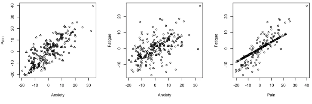
2.6 Data Example
Nephrotic Syndrome (NS) is a common disease in pediatric patients with kidney disease. The typical symptom of this disease is characterized by the presence of edema that significantly affects the health-related quality of life in children and ado-lescents. The PROMIS (Fries et al. (2005); Gipson et al. (2013)) is a well-validated instrument to assess pediatric patient’s quality of life. The instrument consists 7 domains, but here we only choose 3 domains with missing misalignment pattern for illustration. In the data, two QoL measures, pain and fatigue, are measured on two exclusive sets of subjects due to some logistic difficulty at the clinic; out of 226 subjects, 107 subjects have measurements of pain, but no measurements of fatigue, while the other 117 subjects have measurements of fatigue but no measurements of
T able 2.2: Sim ulation results concerning estimation of P earson correlation and marginal regression parameters in the copul a mo del fo r partial ly misaligned missing at random data obtained EM algorithm, compared with the gold standard wit h full data, Multiple Imputation and Hot-Dec k Imputation. (Standard error ratio is calculated b y a ratio of tw o standard errors b et w een a metho d and the gold standard.) F ull Data Copula&EM Multiple Imputation Hot-Dec k Imputation parameter true v alue estimate std.err estimate std.err estimate std.err estimate std.err β10 0 -0. 0012 0.143 0.0596 0.1466 / 0.1488 -0.0012 0.143 -0.0012 0.143 β11 1 1.0030 0.1424 0.9425 0.1451 / 0.1485 1.0030 0.1424 1.0030 0.1424 β12 3 3.0003 0.0496 3.0000 0.0498 / 0.0528 3.0003 0.0496 3.0003 0.0496 σ1 1 0.9975 0.051 1.0446 0.0566 / 0.0522 0.9975 0.051 0.9975 0.051 β20 0 -0. 0050 0.1435 -0.0087 0.189 / 0.2146 -0.0918 0.2134 -0.1405 0.2397 β21 2 2.0049 0.1413 2.0098 0.1864 / 0.2157 2.1654 0.2053 2.1989 0.2104 β22 2 2.0006 0.0514 2.0017 0.0648 / 0.0774 2.0015 0.0719 2.0020 0.0711 σ2 1 0.9977 0.0493 1.0918 0.0883 / 0.0754 0.9836 0.0796 0.9398 0.1046 β30 0 -0. 0023 0.1474 0.1109 0.1915 / 0.1797 0.0503 0. 2178 0.0424 0.2371 β31 3 3.0046 0.1481 2.8902 0.1936 / 0.1776 2.9111 0.2155 2.9160 0.2191 β32 1 1.0010 0.051 1.0005 0.0665 / 0.0634 0.9997 0.0745 1.0006 0.0737 σ3 1 0.9965 0.0508 0.9379 0.0615 / 0.0622 0.9946 0.0752 0.9662 0.0956 γ 0.5 0.5019 0.0408 0.4951 0.0606 / 0.0557 0. 440 9 0.1212 0.4178 0.1149
pain. In addition, two subjects have neither measurements of pain nor measure-ments of fatigue. Interestingly, measuremeasure-ments of anxiety have been fully recorded on all 226 individuals with no missing data. In this case, Hot-Deck imputation does not work. We first apply the complete case univariate analysis of each QoL domain score
(Y1 = anexiety, Y2 = pain, Y3 = fatigue) on covariates of age, gender, edema, race
(white, black, and other as reference), and estimate the linear correlation coefficient of the residuals as 0.6830 between anxiety and pain and 0.5106 between anxiety and fatigue, which turns out to be approximately the square of the correlation coefficient between anxiety and pain. This suggests us use first order autoregressive correlation for matrix Γ in the copula model.
The EM algorithm has two advantages to handle this misaligned missing data pattern. One is that we can estimate both marginal and correlations parameter adjusting for the confounders, where the information across the three QoL scores
can be shared to improve efficiency. The other is the prediction of the missing
QoL scores by using the correlated QoL scores together with the marginal regression
models, which requires the availability of inverse correlation matrix, Γ−1.
The observed data and predicted data from the EM algorithm are all shown in Figure 2.1. The triangles indicate patients with missing fatigue data, and the circles correspond to patients with missing pain data. Between pain and fatigue QoL scores, outcomes have no overlap. The circles and triangles are well distributed and appear to lie in elliptical in the first two scatter plots. In the third plot, the reason that the predicted triangles appear a straight line is the use of AR-1 correlation matrix, and the shape of these points may change to another pattern when a different correlation structure is used.