Similar Language Translation

(1)

Similar Language

Translation

June 25, 2019

Degree’s Thesis

Telecommunications Technologies and Services Engineering

Autor:

Lluís Guàrdia Fernàndez

(2)

(3)

Abstract

Similar Languages are an interesting line of research within Machine Translation since it settles the perfect scenario to exploit the commonalities that present these similar languages. This contrasts other Machine Translation tasks on languages that are more distant and can not exploit such similarities. In this project, we work with the similar languages pairs of Czech-Polish and Spanish-Portuguese.

In this work, we are comparing two of the most popular approaches in automatic translation: statistical and neural-based systems. The latter is the current approach that is used by important companies like Google.

During the project execution, we successfully participated in the 1st WMT Similar Language Translation Task with the submission of the TALP-UPC system using both statistical and neural systems, which was placed 1st for Czech-Polish and 2nd for Spanish-Portuguese in the official evaluation.

To improve the results obtained, it is proposed and analyzed the use of a combination of both systems mentioned with back-translation as a metric measure.

Obtaining in the Spanish-Portuguese case a result 6 BLEU points greater with statistic model than neural, while in Czech-Polish the neural outperforms by 2 BLEU points the statistical. Be-tween both systems, there is a difference of about 40 BLEU points in quality. With the obtained results it is concluded that both analyzed systems achieve very similar results which perfor-mances depend on the language pair analyzed.

Also is inferred that our proposed system combination doesn’t contribute with any substan-tial improvement, actually sometimes it could worsen the obtained results. It is due to back-translation not being able to be considered a good metric to evaluate a back-translation system know-ing, among other reasons, the low correlation values between the quality of the obtained trans-lation and the quality of its back-transtrans-lation.

(4)

pàg. 2

Resum

La traducció de llengües similars és una secció en la traducció automàtica que sempre ha generat interès en recerca per tal de buscar la forma d’aprofitar la similitud que presenten aquestes llengües envers altres de més llunyanes gramaticalment. En aquest projecte es treballa amb els parells de llenguatges similars Xec-Polac i Espanyol-Portuguès.

En aquest treball comparem dos dels enfocaments més populars en traducció automàtica: els sistemes estadístic i neuronal. El segon és l’enfocament utilitzat actualment per grans compa-nyies com Google.

Durant l’execució del projecte també es participa en la 1a Tasca de Traducció de Llengües Simi-lars en WMT amb la submissió del sistema TALP-UPC utilitzant ambdós sistemes, tant estadístic com neuronal, obtenint un 1r lloc en Xec-Polac i un 2n lloc en Espanyol-Portuguès en la avalu-ació oficial.

Per tal de millorar els resultats obtinguts, es proposa i s’analitza l’ús de la combinació dels dos sistemes mencionats utilitzant back-traducció com a mètrica de mesura.

Obtenint-se en el cas Espanyol-Portuguès un resultat 6 punts BLEU major amb el model estadís-tic que amb el neuronal, mentre en Xec-Polac el neuronal supera per 2 punts BLEU l’estadísestadís-tic. Entre els dos sistemes s’obté una diferència d’aproximadament 40 punts BLEU en qualitat. Amb els resultats obtinguts es conclueix que els dos sistemes analitzats obtenen resultats molt simi-lars sent el seu rendiment dependent en gran mesura del parell de llengües analitzades. També s’infereix que la utilització de la combinació de sistemes no aporta cap millora substan-cial, de fet pot arribar a empitjorar, als resultats obtinguts, degut a que no es pot considerar la back-traducció com a una bona mètrica per avaluar un sistema de traducció sabent, entre al-tres raons, la mala correlació entre la qualitat de la traducció obtinguda i la qualitat de la seva back-traducció.

(5)

Resumen

La traducción de lenguas similares es una sección en la traducción automática que siempre ha generado interés en investigación para buscar la forma de aprovechar la similitud que presentan estas lenguas delante otras más lejanas gramaticalmente. En este proyecto se trabaja con los pares de lenguajes similares Xeco-Polaco y Español-Portugues.

En aquest treball comparem dos dels enfocaments més populars en traducció automàtica: els sistemes estadístic i neuronal. El segon és l’enfocament utilitzat actualment per grans compa-nyies com Google.

En este trabajo comparamos dos de los enfoques mas populares en traducción automática: los sistemas estadístico y neuronal. El segundo es el enfoque usado actualmente por grandes com-pañias como Google.

Durante la ejecución del proyecto también se participa en la 1a Tasca de Traducción de Lenguas Similares en WMT con la sumisión del sistema TALP-UPC usando ambos sistemas, tanto el es-tadístico como el neuronal, obteniendo un 1r puesto en Xeco-Polaco y un 2o puesto en Español-Portugues en la evaluación oficial.

Para mejorar los resultados obtenidos, se propone y se analiza el uso de una combinación de los dos sistemas mencionados usando back-traducción como métrica de mesura.

Obteniéndose en el caso Español-Portugues un resultado 6 puntos BLEU mayor con el modelo estadístico que con el neuronal, mientras en Xeco-Polaco el neuronal supera por 2 puntos BLEU el estadístico. Entre los dos sistemas se obtiene una diferencia de aproximadamente 40 puntos BLEU en calidad. Con los resultados obtenidos se concluye que los dos sistemas analizados obtienen un resultado muy similar siendo su desempeño dependiente en gran mesura de el par de lenguajes analizados.

También se infiere que la utilización de la combinación de sistemas no aporta ninguna mejora substancial, de hecho puede llegar a empeorar, a los resultados obtenidos, debido a que no se puede considerar la back-traducción como una buena métrica para evaluar un sistema de traducción sabiendo, entre otras razones, la mala correlación entre la calidad de la traducción obtenida y la calidad de su back-traducción.

(6)

pàg. 4

Acknowledgments

First I want to thank my tutor Marta R. Costa-Jussà for guiding me through this project and giving me the opportunity to participate in a task presented internationally, and Magdalena Biesialska. who was part of the project too and without her would have been impossible to finish it. It was a pleasure to work with you.

I want to thank my parents for all the support, dedication, affection and all the invaluable things they gave me during all my life.

Thanks to all my colleagues who worked with me during this long five years either in the lab-oratory or theoretical classes. All names couldn’t fit in this page but I want to thank especially Xavier Barrera and Oriol Barbany, who had been in almost every laboratory class during this last two years.

And finally, I want to thank Maria, who has infinite patience for bearing me and listening all my verbosity for the lasts months, and was at my side whenever I needed it.

(7)

Revision history and approval record

Revison Date Purpose

0 20/05/2019 Document creation

1 21/06/2019 Document revision

2 24/06/2019 Document approbation

DOCUMENT DISTRIBUTION LIST

Name e-mail

Lluís Guàrdia Fernàndez [email protected] Marta R. Costa-Jussà [email protected]

Magdalena Biesialska [email protected]

Written by: Reviewed and approved by:

Date 20/05/2019 Date 24/06/2019

Name Lluís Guàrdia Fernàndez Name Marta R. Costa-Jussà

(8)

pàg. 6 CONTENTS

List of Figures

1 Gantt Diagram. . . 12

2 Noisy channel concept . . . 14

3 Basic concept of Beam Search . . . 15

4 Basic schema of a Phrase-based MT system . . . 17

5 Structure of a perceptron . . . 19

6 Operations AND, OR and XOR as linear separation problems . . . 19

7 Diagram of an RNN. . . 20

8 Attention mechanism concept . . . 21

9 Back-translation selection approach. . . 25

(10)

pàg. 8 LIST OF TABLES

List of Tables

1 Alphabet size in European languages [Leira] . . . 10

2 Specifications of the cpu’s in CALCULA machines . . . 11

3 Results comparison between word and phrase based. . . 16

4 Wheights in an attention mechanism example . . . 21

5 Results obtained for the example candidate . . . 22

6 Number of sentences used . . . 26

7 Phrase-based (PB) and Neural-based (NMT) results . . . 32

8 Results in the WMT evaluation . . . 32

9 Back-translation systems results . . . 32

10 System Combination Results. . . 33

11 Correlations and BLEUs for the various combinations.. . . 34

12 Correlation between translation and back-translations . . . 34

13 Language Distances within some Slavic, Romance and across languages families. 35 14 Total cost of the salaries . . . 37

15 Office expenses cost . . . 37

16 Final cost consumption of electricity . . . 38

(11)

1 Introduction

From long to the past, humans are interested in the possibility of communicating in an auto-matic way between different languages, from Johan Joachim Becher on 1661, with the first MT resembled approach system [Becher1962], until the more recent Alan Turin, and his decipher-ment of the German Enigma machine, during WW2 [Lee1997].

Since a few years ago, especially thanks to the progress on Machine Learning, the increased number of source texts available in more and more languages from the internet and the im-provement on accessibility, both for companies and consumers; the Machine Translation (MT) systems have been improving a lot, and they still do it today, having the translation of docu-ments without the help from any other person as their goal.

In the last years, the similar language translation may have started to wrongly been considered as a solved task, which, as the name indicates, consist of translating languages that are more close due to their similar point of origin, and are more easy to translate (like the Spanish and Portuguese). That is mostly due to the great results obtained by the MT systems.

These MT systems are automatic translation systems or “translation carried out by a computer”, as defined in the Oxford English dictionary. In a very summarized form: it’s a process some-times referred to as Natural Language Processing [Weiscbedel et al.] where you input a text in a certain language to the computer and, in result, it gives you the text translated to the target language.

However, there are still some challenges to surpass that will lead to a better system performance in the future, such as limited resources to some of the less known languages, out-of-domain, or the difference between alphabets used in both languages, even at similar languages, as you could observe at Table11 2_.

Within this systems, the most distinguished for its results is the Neural MT [Vaswani et al.2017], which uses Deep Learning to generate, using the source texts, information vectors for each word associating information of the words surrounding it, capturing a great amount of information Despite this, for some of the tasks, statistical approaches are still competitive [Lample et al.2018].

1_{There are two versions of the Hungarian alphabet, one which is said to be official (also characterized as ’full’} or ’old’). The other one is said to be taught in school and is characterized as ’strict’ or ’standard’. In this case we are referring to the full version

2_{The alphabet doesn’t include the letters with diacritics where the resulting letter is considered an ordinary letter} in the alphabet of the language where it is used

(12)

pàg. 10 1. INTRODUCTION Alphabet Langauge

26 Standart European

21 Italian

23 Portuguese

26 EnglishGerman FrenchIcelandic Irish

27 Finnish

29 DanishNorwegian SwedishFarese

Turkish Sami

30 Spanish Croatian

31 Czech Romanian

32 Estonian_Polish Lithuanian

33 Latvian

36 Albanian Bosnian

44 Hungarian

Table 1: Alphabet size in European languages [Leira] 1.1 Statement of purpose and contributions

The main goal of the project is to test which system among neural or statistical MT is better for close languages with limited results, implementing these statistical and neural MT, and partici-pate in the 1st Similar Language Translation WMT task for the Czech-to-Polish and Spanish-to-Portuguese translation directions. The main contribution is the implementation of a statistical MT with Moses [Koehn et al.2007] system which ranked second in the Similar Language Trans-lation Shared Task in the Fourth Conference on Machine TransTrans-lation (WMT19). Also the usage of the techniques of back-translation and minimum Bayes risk [Kumar and Byrne2004] in order to evaluate the translations.

1.2 Requirements and specifications

This project has been developed in two differentiated parts, that were combined in the last sec-tions. For the Neural MT was used the open-source Fairseq architecture3_{which required}

Py-Torch version greater or equal than 1.0.0 and Python version greater or equal than 3.6. And for the statistical MT, we used the open-source Moses toolkit v4.0. 4

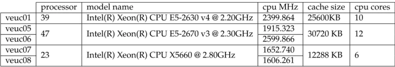
All the software has been launched in the CALCULA cluster, which consist of 8 servers from the TSC department of the UPC, each with 2 IntelR©XeonR©E5-2670 v3 2,3GHz 12N processors,

3_{https://github.com/pytorch/fairseq}

(13)

and a total of 16 NVIDIAGTX Titan X GPUs. Each GPU has 12GB of memory and 3072 CUDA Cores. Among those servers, there was a great heterogenous variety of CPU’s for this task due to the difference of ages of them. The specifications for them are in the table2:

processor model name cpu MHz cache size cpu cores

veuc01 39 Intel(R) Xeon(R) CPU E5-2630 v4 @ 2.20GHz 2399.864 25600KB 10 veuc05 47 Intel(R) Xeon(R) CPU E5-2670 v3 @ 2.30GHz 1915.323 30720 KB 12

veuc06 2599.866

veuc07 23 Intel(R) Xeon(R) CPU X5660 @ 2.80GHz 1652.740 12288 KB 6

veuc08 1606.261

Table 2: Specifications of the cpu’s in CALCULA machines 1.3 Methods and procedures

This project main idea was originally proposed by my supervisor and it didn’t come from any previous work. It is a combined effort between me and Magdalena Biesialska, who carried out the Neural MT tasks.

In this project, the neural model is based on the Transformer architecture implemented by Face-book in the Fairseq toolkit. The transformer is the most current state-of-the-art NMT architec-ture [Vaswani et al.2017] which relies solely on the self-attention mechanism and shows signif-icant performance improvements over traditional sequence-to-sequence models.

The statistical model is based on a Phrase-based structure implemented by the open-source Moses toolkit, which is one of the most widely used Statistical MT Application.

The majority of the coding during this project was written in Bash scripting. 1.4 Work Plan

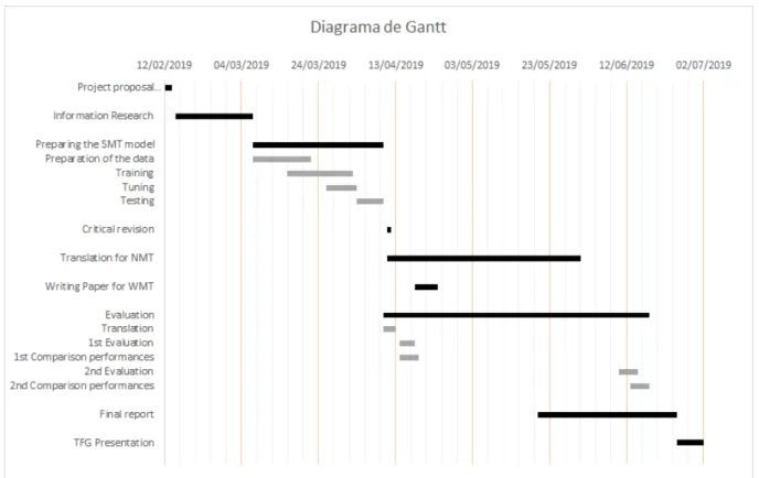
The project was structured in the Work Packages exposed below and the Gantt Diagram. • WP 1: Project propose and work plan

• WP 2: Information research

• WP 3: Preparing the SMT model (Moses) · data preparation

· building the system

• WP 4: Translation for NMT model5

(14)

pàg. 12 1. INTRODUCTION • WP 5: WMT Paper6 • WP 6: Critical review • WP 7: Evaluation • WP 8: Final Report • WP 9: TFG presentation

Figure 1: Gantt Diagram 1.5 Incidences

In order to use as a pseudo-corpus for the Neural MT we needed to translate the corpus using the Statistical MT, this process took more memory and time that we had expected. As it was a huge corpus, it also took more time to train the Neural MT system. Due to this, for the Spanish-Portuguese language pair, we were unable to finish training our NMT model with the pseudo corpus (Table7).

In the SMT case, the translation rate was normally approximately 2000 sentence/hour, but it un-dulates between 500 and 3.000 depending on which server was allocated within the CALCULA cluster.

(15)

2 WMT Task

In this section we explain the shared task in which we participated.

The shared task: Similar Language Translation7_{is proposed for the 4th Conference on Machine}

Translation (WMT), which will be held on August 1-2, 2019, in Florence, Italy. It is organized by Costa-jussà, M. from Universitat Politècnica de Catalunya, Malmasi, S. from Harvard Medical School, Pal, S. from Saarland University, and Zampieri, M. from University of Wolverhampton. WMT started in 2005 and, since then, a wide range of shared task related to translation has been carried out. From translation of news, up to unsupervised translation, through translation using system combination and others.

A shared task consists of a challenge provided by the organizers with the training data attached, it has to be remarked that it is a combined effort to improve and research in the field, not a competition between the participants. Then, on a pre-announced data, unseen test sets are released for the use of participants, which will have to submit the system results given these sets. Finally, the results are published and the evaluation and techniques are presented in a conference.

For the first time in WMT, a shared task in "Similar Language Translation" is organized. The objective of this task is to evaluate the performance of the translation between pairs of similar languages from the same language family, using state-of-the-art translation systems.

In the increased use of MT technologies, there is also an increased interest in training the sys-tems between languages different than English, since in automatic translation it is, by far, the most used language, due to the great quantity of training data and resources available. The vast majority of MT systems look for translation from/to English or, in case of translation of languages with a shortage of resources available, it is used as the pivot language.

The fact that English is not used in any of the languages for/to translate supposes a lesser quan-tity of parallel data available for the task. In order to overcome this limitation, it’s necessary to find a way to take advantage of the similarity between the pair of languages in a direct transla-tion of similar languages.

The evaluation in this task will be carried out using automatic evaluation metrics. All systems are ranked by BLEU score [Papineni et al.2002], and TER score [Snover et al.2006] will be calcu-lated for systems with BLEU scores greater than 5.0.

In this task are only allowed submissions which only uses the parallel data provided (con-strained) for training, no additional parallel data is allowed. With monolingual data, you are encouraged to develop novel solutions to improve translation quality.

All participants will be provided with training and testing data for 3 pairs of languages:8

• Spanish - Portuguese (Romance languages) • Czech - Polish (Slavic languages)

• Hindi - Nepali (Indo-Aryan languages)

7_{http://www.statmt.org/wmt19/similar.html} 8_{in this project only the two first will be used}

(16)

pàg. 14 3. BACKGROUND

3 Background

In this section, we overview the statistical (phrase-based) and the neural-based MT approaches that we use in this study, and the evaluation metric used, the BLEU score.

3.1 Statistical Machine Translation

Statistical MT translations are based in the statistic model and information theory, it could be that the probability of a word combination in the source language could be calculated from the statistic relationships between this words, extrapolating these relationships from the aligned corpus9 _{from bilingual texts (a famous example of this kind of bilingual text is the Rosetta}

Stone), as Jordan, Dorr and Benoit express [Dorr et al.1998]. This approach contrasts with pre-vious traditional approaches like the automatic translation based on rules, which were used to express translation knowledge, or based on examples.

Although the SMT approach is considered to be first proposed in 1990 by Peter F. Brown [Brown et al.1990] and being a hot topic since then, the first to suggest the application of the ideas of statistics models and information theory to the machine translation field was W. Weaver at 1949 [Weaver1995], but it didn’t draw the attention until it was reintroduced by Brown and the IBM researchers.

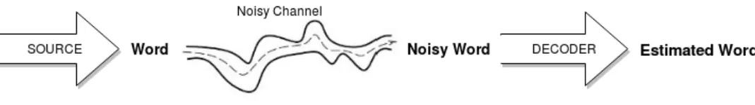
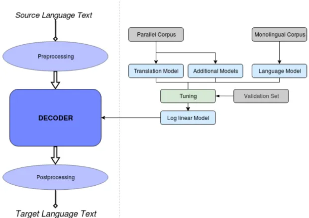
The researchers from the T.J. Watson research center with IBM were the first to propose an SMT based on source channel model [Brown et al.1993], also called noisy channel model (Figure 2). This process is divided into three sub-problems: the modelling of a language model, the modelling of a translation model and decoding.

Figure 2: Noisy channel concept

Using the Bayes rule to reformulate the translation probability for translating a source sentence sinto the target languagetas:

argmaxtP(t|s) =argmaxtP(t)P(s|t)

P(t)is the language model, which takes care of the fluency in the target language. It is obtained through monolingual corpora in the target language. Basically, it estimates how probable a sentence is, but it has problems such as zero probability in long chains, since it is difficult to observe them in the corpora. The solution to this problem is using the n-gram approach [Kneser and Ney1995]. It consists in considering the probability of a sentence as the product of the conditional probabilities of each word. For example, using a 3-gram model:

(17)

The girl was upset.

P(t) =P(T he_|φ, φ)_∗P(girl_|φ, T he)_∗P(was_|T he, girl)_∗P(upset_|girl, was) (1) However, with this approach long-range dependencies are lost, and some n-grams can be not observed in the corpora, so smoothing techniques such as linear interpolation or back-off mod-els are required.

Then,P(s_|t)is the Translation model, which is an estimation of the lexical correspondence be-tween languages and it’s obtained through the aligned bilingual corpora in both, source and target languages To generate this model, it should take into account for each word in the source language its translation, the number of necessary words in the target language, the position of the translation within the sentence and the number of words that need to be generated from scratch. In conclusion, its quality depends on the obtained word alignment, and we can esti-mate it with the statistical model (counting probabilities in a huge corpus) but the corpus is not aligned word by word. In this case, we could estimate word alignments together with the parameters used [Och et al.1995] or we could apply the phrase-based approach.

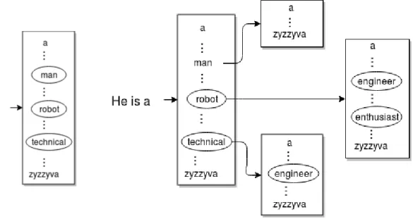
Finally, theargmaxtpart is done by the decoder. Once we have the given models (Language Model, Translation Model or others), the decoders are responsible for constructing the possible translations and searching the most probable one. There are some possibilities for this search, the most efficient and used one being beam search [Koehn et al.2003] along with cube pruning [Chiang2007].

This heuristic consists in store the B top possible word translations, whereB is a threshold parameter. Then repeating this process but only to the stored options. This approach allows saving a lot of memory by not going down all the possible translations. You can see a scheme of it in figure3.

(18)

pàg. 16 3. BACKGROUND This source channel method was the most used and studied for automatic translation, until 2016, where it began to be replaced by the neuronal MT.

From the linguistic knowledge perspective, the framework can be classified into three models: word-based, phrase-based and syntax-based. The most usual, being used by companies like Google, IBM, ISI and others; and the one that we will focus on in this project is the phrase-based.

3.1.1 Phrase-based approach

Phrase-based statistical MT [Koehn et al.2003] uses the noisy channel model but, unlike the word-based approach which translates word by word, translates by concatenating at a phrase level the most probable target given the source text.

Source The enemy team gave up Word-based El equipo enemigo paso arriba Phrase-based El equipo enemigo abandono

Table 3: Results comparison between word and phrase based

In this context, a phrase is a sequence of words, ignoring if it’s a phrase or not from a linguistic point of view. Phrases are extracted based on the probabilistic study of a large parallel corpus, which identifies and ranks each phrase with several features, such as conditional probabilities. The collection of scored phrases constitutes the translation model.

This approach seems like a closer take to the syntax of the languages, and so allows improve on the word-to-word translation, and the phrase-learning helps to resolve ambiguities, as context can provide useful clues about translation.

In order to calibrate the output size in this approach, a W factor is introduced, which corre-sponds to the word cost, for each generated word in the target language [Koehn et al.2003]. So the formula remains as:

argmaxtP(t|s) =argmaxtP(t)P(s|t)wlength(t)

In addition to the models mentioned previously, there are also other models to help achieve a better translation, such as the reordering model, which helps in a better ordering of the phrases. The weights of each of the models are optimized by tuning over a validation set. Based on these optimized combinations, the decoder uses beam search to find the most probable output given an input. Figure4shows a diagram of the phrase-based MT approach.

(19)

Figure 4: Basic schema of a Phrase-based MT system 3.2 Neural Approach10

Neural Networks for MT scientific papers started appearing around 2014 [Bahdanau et al.2014], and are very successful since then, helped by a great number of advances in recent years. The first appearance of NMT systems in an MT public competition was in 2015 (OpentMT’15). And at the OpenMT’16 the following year, 90% of the winners were NMT systems [Bojar et al.2016] showing a similar or even better performance than the phrase-based SMT systems [ Kalchbren-ner and Blunsom2013, Cho et al.2014, Sutskever et al.2014, Bahdanau et al.2014, Sennrich et al.2016a,Zhou et al.2016,Wu et al.2016].

NMT derives from SMT phrase-based approaches [Wołk and Marasek2015] and uses large ar-tificial neural networks, its great difference is the use of vector representations or embeddings for words and internal states. The structure is more simple than phrase-based models since there is no separation between the Language Model, Translation Model and Reordering Model, just one sequence model that predicts one word at a time. However, this sequence predictor is conditioned by the entire source sequence and the already translated part.

Actually, the most predominant NMT model used is the bidirectional RNN provided with a Long-Short Term Memory (LSTM) units [Hochreiter1997] or Gated Recurrent Units (GRU) [Cho et al.2014] in both encoder, which is used to encode the source sentence, and decoder, which 10_{Even though I didn’t participate in this part, I feel necessary to explain it since we did use its translations results}

(20)

pàg. 18 3. BACKGROUND does the word prediction in the target language [Bahdanau et al.2014]; combined with an at-tention mechanism [Luong et al.2015]. Other approaches, although less usual, are used for sequence modelling such as Convolutional Neural Networks (CNN) [Kalchbrenner et al.2016, Gehring et al.2017].

In this project we will focus on one of the more current architectures, the Transformer [Vaswani et al.2017], which shows an important improvement over sequence-to-sequence traditional mod-els. In spite of using some earlier concepts used in RNN-CNN based models such as residual connections [He et al.2015] or position embeddings [Gehring et al.2017].

Since 2016, the majority of the best MT are using Neural Networks [Bojar et al.2016] such as Google, Microsoft, Yandex, among other translation services. An open source neural machine translation system, OpenNMT, has been released by the Harvard NLP group [Klein et al.2018]. 3.2.1 Artificial Neural Networks

Artificial neural networks (ANN) are a type of machine learning algorithm inspired by the func-tioning of biological neurons in animals brains. Such systems "learn" to perform tasks by con-sidering examples, generally without being programmed with any task-specific rules.

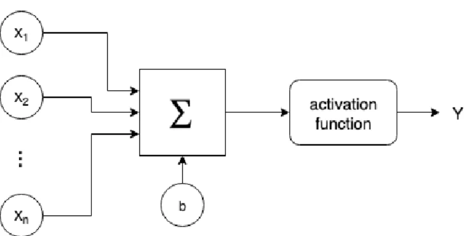
They normally consist of a group of basic processing units called artificial neurons (AN) or per-ceptrons (Figure5) which are wired together in a complex communication network. They can compute an output given input data by decomposing it in different representations in order to identify different characteristics.

Each AN model is a simplified model of a real neuron, which sends off a new signal if it receives strong enough input signal from the other nodes to which is connected, allowing it to perform some basic operations such as AND, OR or NOR.

This model was first proposed by Warren McCulloch and Walter Pitts in 1943 [McCulloch and Pitts1943]. Among many other proposed models, the most simple AN architecture was the per-ceptron [Rosenblatt1961], which improves the usage of binary values for the McCulloch and Pitts model to being operational with any numbers. It works through an algorithm that com-putes the so-named activation function:

ouput=f(X ∀i

wixi+b) (2)

Where wi are the weights of the input values xi andb is a bias, used to give some extra de-gree of freedom. These values are computed using gradient descent techniques [Barzilai and Borwein1988], which consist in taking proportional steps to the negative of the gradient of the function iteratively at the current point, so it approaches the global minimum of the function.

(21)

Figure 5: Structure of a perceptron

The output (Y in Figure5) has an internal threshold, so the output values of the perceptron are binary and they depend on if the output of the activation function exceeds or not this thresh-old. This allows the perceptron to linearly separate samples into two classes, that’s why it can compute basic operations like AND or OR, but not non-linear separable functions or problems like XOR (Figure6).

Figure 6: Operations AND, OR and XOR as linear separation problems

To solve this more complex structures are needed. One basic neural network structure, among many others, is the Multilayer Perceptron (MLP), which basically consist of multiple layers of perceptrons.

The basic structure consists of 3 layers of nodes: the hidden layers for multiple representations of data and characteristic identification, these layers are fed with all the data by an input layer, and finally the output layer, which can use a different activation function depending on the nature of the task.

Adding Monolingual Data. Differently, from the statistical MT approach, the neural MT ap-proach does not include monolingual data in the standard training. However, previous studies have reported notable improvements by adding monolingual corpora through back-translation [Sennrich et al.2016b].

(22)

pàg. 20 3. BACKGROUND 3.2.2 Recurrent Neural Network

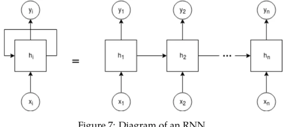
Recurrent Neural Network (RNN) is a type of ANN formed by a sequence of concatenations of the same unit along a temporal sequence (Figure7), this structure allows them to retain infor-mation from previous data like a temporal memory. This approach is used in the majority of NMT models today and were based on David Rumelhart’s work in 1986 [Williams et al.1988].

Figure 7: Diagram of an RNN

Due to its capacity to retain information, they are pretty useful for sequential data, where each element of the sequence could be related to others.

Another type of RNN with improved long term dependencies are the LSTM [Hochreiter1997], which, due to its internal structure formed by four operation layers unlike the just one used by conventional RNN, can perform different operations such as update, forget or output informa-tion. A variant of the LSTM are the Gated Recurrent Unit (GRU) [Cho et al.2014], which have a simpler structure, making them computationally more efficient and faster to train.

These are the more common RNN in NMT, however, all of them suffers from the vanishing gradient problem, which means that they are losing more information as "time" passes.

3.2.3 Transformer

One architecture proposed that don’t suffer from memory loss is the Transformer [Vaswani et al.2017], which relies only on the attention mechanism without resorting to recurrence nor convolution [Luong et al.2015].

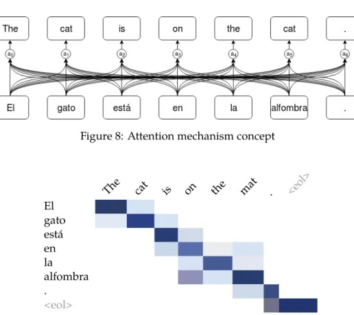
The attention mechanism looks at the input sequence and decides at each step which other parts of the sequence are important by giving them different weights (Figure8) that will be used by the decoder as shown in Figure411_.

Summed up, each word receives an attention weight normalized between 0 and 1, which is defined by how each word of the sentence is influenced by all the other words in the sequence.

(23)

Figure 8: Attention mechanism concept

The cat is on the mat . <eol> El gato está en la alfombra . <eol>

Table 4: Wheights in an attention mechanism example

In the variant used in this project of the implemented self-attention by the Transformer, the rep-resentation of a word given is produced by means of computing a weighted average of attention scores for all the words of a sentence.

3.3 BLEU score

Imagine you have a Spanish sentence, and you are given a human-generated translation of it as a reference. However, there could be multiple sentences considered perfectly good translations of that Spanish sentence.

The Bilingual Evaluation Understudy or BLEU [Papineni et al.2002] is a method to evaluate the quality of a machine-translated text. The basic idea behind BLEU is that, the closer a ma-chine translation is to a professional human, the better it is. BLEU allows using more than one reference, which allows better robustness.

In order to illustrate better how the BLEU score works we will use an example, with the Spanish sentenceEl gato está en la alfombraas the sentence to translate. As a human reference, we have

gotten two accepted translations, the first beingThe cat is on the mat, and the second being There is a cat on the mat.

What BLEU method does is, given a machine-translated text, it computes a BLEU score that measures how good that MT is. The more basic intuition behind the BLEU score is to look at the machine-generated output and see if the words it generates appear in the human-generated

(24)

pàg. 22 3. BACKGROUND references. So, if we look at each word in the MT output and see if it appears in the references, we are calculating the precision of the MT output, which is a number between 0 and 1.

However, in order to resolve some deficiencies, it’s normally used the modified precision mea-sure in which we will give each word credit only up to the maximum number of times it appears in the reference sentences. Also, as we don’t want to just look at isolated words, we will look at n-grams (a group of n consecutive words).

And so the algorithm goes as follows:

• First, we will count the number of distinct n-grams in the candidate.

• Then we will count the number of times each n-gramgioccurs in each reference. But we will only take the maximum of each of these values calculated.

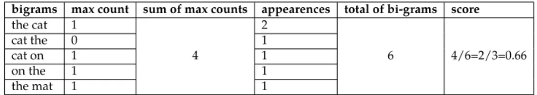
• Finally, we will add the maximum calculated previously of each n-gram, and divide them by the total number of n-grams in the candidate (this time they don’t have to be distinct). So to start with the example, we get the slightly good translationThe cat the cat on the matas

an MT output, and we will evaluate it using bi-grams.

Candidate: The cat the cat on the mat Reference1: The cat is on the mat Reference2: There is a cat on the mat

bigrams max count sum of max counts appearences total of bi-grams score the cat 1 4 2 6 4/6=2/3=0.66 cat the 0 1 cat on 1 1 on the 1 1 the mat 1 1

Table 5: Results obtained for the example candidate

So, in this example, we get that the sum of each bi-gram maximum number of appearances in the references is 4. And, although we have 5 distinct bi-grams in the candidate, the number of total bi-grams is 6 asthe catappears twice. In result, we obtain a score of 4/6 or 2/3.

So we could compact all of this in the formula3where the subscriptnindicates for what number of n-grams are we calculating andyis the MT output or candidate. :

pn= P

n−grams∈ymax count of appearances in reference P

n−grams∈ytotal n-grams in candidate

(3) Finally, to obtain the final BLEU score, we calculate the Combined BLEU score (Formula 4) which is the value of all the n-grams modified precision. Where we basically exponentiateeby the mean of values from unigrams to 4-grams and multiply it by BP, which stands for brevity penalty (Equation5) and is an adjustment factor that penalizes translation systems that output translations that are too short.

(25)

score=BP _∗exp(1 4 4 X n=1 pn) (4) BP = (

1 iflengthy ≤lengthref erence exp(1₋ lengthy

lengthref erence) otherwise.

(5) BLEU score was revolutionary for machine translation because it gave a, by no means perfect, but pretty good single real number evaluation metric.

In practice, BLEU was one of the first metrics to claim a high correlation with human judgements of quality [Coughlin2003] and remains one of the most popular automated and inexpensive metrics. And so there are multiple open source implementations that you can download and use to evaluate your own system (Moses multi-bleu.perl script, NIST mteval-vXX.pl script, etc), but it’s recommended to stick with only one per project since they have different implementations and their results may differ between them.

(26)

pàg. 24 4. RELATED WORK

4 Related Work

In this section it is explained a little overview of previous works related to the project.

A considerable quantity of works have been developed lately associated with similar languages, due to the less complexity of them against non-similar languages. Even so, a great part of them are more related to the task of distinguishing between them more than translation.

West Slavic languages, which is the case for Czech and Polish, had never been a great focus of interest in research partly due to the shortage of resources available. Lately, several systems have been implemented more focused in the translation of a third, more international, language such as English [Kirschner1987,Wolk and Marasek2014] or Russian [Bémová and Kubon1990] than in the translation between them.

In the Czech-Polish case, we find that there is a minimum of translation systems. The majority of them are about Czech-Slovak since the great similarity between both of them. Even so, some works focused on Czech-Slovak were searching for a multilingual implementation with the rest of languages within the same family, such is the case of the Kubon, V. work [Hajič et al.2000], in which they were searching for an implementation using more simple methods, following a word-for-word approach.

In the case of the romance languages, Spanish and Portuguese within them, we can find more cases of direct translation systems between similar languages, but mostly in Spanish Catalan, due to its great translation results [Alonso2005].

One approach in Catalan-Spanish taken by interNOSTRUM [Canals et al.2019] and Sishitra [Navarro Cerdán et al.2004], along with other few papers in other pair of languages such as one from Irish to Gaelic Scottish [Scannell2006], were more focused towards exploring similarities in varieties, dialects and closely related languages consisting of a pipeline of different components such as a Part-of-Speech tagger (POS-tagger) or a Naïve Bayes word sense disambiguator. In the more specific case of Spanish-Portuguese, Garrido-Alenda used a word-for-word MT refined by shallow parsing techniques [Garrido-Alenda et al.2003].

We can find more classical approaches like a rule-based system [Grazina et al.2011] or phrase-based and neural systems [Costa-jussà et al.2018] in translating between Brazilian Portuguese and European Portuguese. Also in Spanish-Portuguese a phrase-based system for broadcast news [Martínez et al.] or medical terms [Renato et al.2018].

With system combination, we could found a great variety of implementation like the CMU [Hildebrand and Vogel2009] or RWTH system combination [Leusch et al.2009], but in any of them, there is in consideration the usage in similar languages, where the phrase-based can offer more competitivity against neural.

Even though we found a similar approach in the work of Costa-Jussa, M.R. [Costa-jussà2017], where it’s applied neural, rule and phrase-based systems in Catalan Spanish pair and use an MBR system combination, it takes some different ways as it doesn’t use back-translation and so the system combination is not applied over them, and NMT uses an RNN with attention and doesn’t add monolingual data.

In none of them, we found an application of a Neural MT or a system combination in the Spanish Portuguese or Czech Polish case.

(27)

5 System Combination with backtranslation

In order to achieve the best possible result in the translations, we propose to combine the results of both phrase-based and NMT systems at a sentence level so that we choose the better case for each of the sentences of the translated text. We aimed for a relatively simple combination strategy comparing with other previous work [Marie and Fujita2018].

The principle of this approach consists in the evaluation of the back-translations generated by both systems using the BLEU score [Papineni et al.2002], choosing the sentence that obtained better results. To obtain a score out of the translations texts, since. theoretically, we don’t have a reference, we back-translated (translate again and obtain a text in the original language) each of the translations using both PB and NMT systems, instead of using only one, and weighted them equally. A graphical representation of this strategy can be found in Figure9.

The final translated text is composed by each of the sentences from the system that obtained the highest score in the combined back-translation in each case.

Figure 9: Back-translation selection approach

This approach is motivated by the recent success of different uses of back-translation in neural MT studies [Sennrich et al.2016b,Lample et al.2018].

Contrastive approaches We thought that to evaluate better the results obtained will be good to have some contrastive approaches, thus we decided to use MBR, which uses the translations instead of the back-translation, and length ratio, which doesn’t consider the content of the sen-tences translated, as contrastive measures.

Minimum Bayes Risk [Kumar and Byrne2004] as said by Kumar, S. and Byrne, W. "consist in apply the techniques with the same name developed for automatic speech recognition [Goel and Byrne2000] and bitext word alignment for statistical MT [Kumar and Byrne2002] to the the problem of building automatic MT systems tuned for specific metrics". It aims for the solution that carries the least Bayesian risk since we are training and decoding with imperfect models. The length ratio is a simple yet not content-based evaluation method since the premise is to calculate the ratio between the number of words in the input and output translated sentences. With this approach we are assuming that a good back-translation will be the one that contains the same numbers of words, regardless of which ones, as the source sentence.

(28)

pàg. 26 6. IMPLEMENTATION

6 Implementation

In this section, we report details about the data and preprocessing, the steps taken with Moses in order to configure the translation system and the parameter details of the systems and system combination.

6.1 Data and Preprocessing

Both systems, statistical and neural, use the corpora (monolingual or parallel) provided by the organizers, no external dataset is used. For both Czech-Polish and Spanish-Portuguese, we used all available parallel and monolingual data [table6].

idiom sentences parallel corpus es-pt_cz-pl 2.481.441_2.191.379 monolingual corpus

es 46.257.689 pt 10.376.328 cz 73.090.126

pl 1.197.480

validation corpus all 3.000

test corpus es-pt_cz-pl 3.000_3.412 Table 6: Number of sentences used

Regarding the validation set, we split it into two parts, the first, consisting of 2 thousand sen-tences, was used as additional training data, and the remaining part, consisting of 1 thousand sentences, was used as validation. Our test set corresponds to the official evaluation set. The postprocessing of the test set once translated, was done in reverse order and included de-truecasing and detokenization.

6.1.1 Moses

Moses allows to adjust its functioning in different ways and offers a great variety of functional-ities. Although we implemented a bidirectional system, in this section I will explain the steps used in order to implement a unidirectional Spanish-Portuguese Phrase-based translation sys-tem with moses12_.

In this section, we will use the parameters $my_dir, as the personal directory of the user, and $moses_dir, as the ubication of Moses and all its tools. Also, we will use the following corpus:

12_A _more _extensive _{documentation} _can _be _found _in _the _Users _Manual _in http://www.statmt.org/moses/manual/manual.pdf

(29)

• the parallel corpus, ascorpusp

• the monolingual and first 2k sentences of the validation will be merged in a sole corpus in order to have a bigger training corpus and improve the results, naming itcorpustraining

• the remaining 1k sentences of the validation as adev1kfile • a corpus combining all the other corpus namedcorpusall Corpus Preprocessing

We have a folder "corpus" where all the corpus are stored and, as all we will do in this part will be in preprocessing level, all the steps taken in this subsection will be done being inside this directory.

cd $my_dir/corpus

• Tokenize:

The first step‘13 _{is to normalize and tokenize, which means to separate the sentences in}

order to have every word and punctuation mark surrounded by spaces, all the sets of data that we will be using during the project.

$moses_dir/scripts/tokenizer/normalize-punctuation.perl -l pt < \ corpusp.pt | $moses_dir/scripts/tokenizer/tokenizer.perl -l pt > \ corpusp.tok.pt

The same process is needed for all the other corpus (corpustraining, dev1k and corpusall). • Truecase:

Lita, L.V. defines truecasing as "the process of restoring case information to badly-cased or non-cased text" [Lita et al.2003].

In order to help Moses know which words should truecase we have to train a Truecaser. This Truecaser is global for all corpus and will have better results as more data we input, so we will use the corpusall corpus prepared before.

$moses_dir/scripts/recaser/train-truecaser.perl -model \ truecase-model.pt -corpus corpusall.tok.pt

When we have the Truecaser trained, we truecase all the corpus except the corpusall, which from now on will no longer be needed.

$moses_dir/script/recaser/truecase.perl -model truecase-model.pt < \ corpusp.tok.pt > corpusp.tok.truecase.pt

13_{we take for granted that you have two correctly differentiated corpus, monolingual and parallel, for each of the} two languages used in the translation

(30)

pàg. 28 6. IMPLEMENTATION • Cleaning

The last step in the preprocessing is to clean all corpus, which means to delete all the sentences wrong aligned or too large. We defined the maximum length of a sentence to be 50 words.

$moses_dir/scripts/training/clean-corpus-n.perl corpusp.tok.truecase \ es pt namecorpus.clean 1 50

And with this, we finished the preprocessing of the data. Language Model

To continue, we return to the original directory. cd $my_dir

Now we have to generate the language model (explained in3.1). Moses normally uses a lan-guage model based on the target lanlan-guage paralel corpus, but we added the training corpus in a new corpus named corpusmodel since using additional training data is often beneficial. Moses also gives different options to construct the Language Model such as RandLM, KenLM or OxLM. We used a 5-gram KenLM since is fast and use low memory.

We create a new directory to store all files related to the LM. mkdir $my_dir/lm

$moses_dir/bin/lmplz -o 5 -T /tmp < corpusmodel.pt > lenguagemodel.arpa.pt Once the model is done, we binarize it as this changes help to reduce loading time.

$moses_dir/bin/build_binary lenguagemodel.arpa.pt lenguagemodel.blm.pt

Even though is not strictly necessary, in our case we wanted to reduce the memory used to translate since we had some delays regarding the need of more memory, but it depends on the computer used and the size of the file to translate. In order to do that we applied two commands: We tried to reduce the memory used by the LM. As a trade-off, we take more time to extract the LM but using less memory. This was accomplished doing:

bin/build_binary -a 64 trie languagemodel.arpa.pt languagemodel.blm.pt

We also used on-demand loading, in order to avoid loading the full LM into memory at the beginning. In order to do that we had to modify the line KenLM inside [features] from the moses.ini file created after the training, adding lazyken=true.

(31)

Training

Now we arrive at the training part. The command used consists of various functions such as word alignment in order to have an adequated corpus for Moses, phrase extraction and punc-tuation or the creation of the configuration file moses.ini. All of the halfway files and final configuration such as the moses.ini configuration file will be stored in a new directory named traines-pt.

mkdir $my_dir/traines-pt

$moses_dir/scripts/training/train-model.perl -root-dir $my_dir/traines-pt \ -corpus $my_dir/corpus/corpustraining.clean \

-f es -e pt -external-bin-dir $moses_dir/tools -mgiza \ -alignment grow-diag-final-and \

-reordering msd-bidirectional-fe \

-lm 0:5:$my_dir/lm/lenguagemodel.blm.pt:8 -parallel > training.pt.out 2>&1 In our case, this part took 9 hours more or less to be finished, but again it depends on the computer capacity and the corpus size used.

Tuning

Finally, in order to calibrate and optimize the translation system, we apply the tunning, which in summary readjusts the word weights having in count the corpus used as validation, in our case the file dev1k. This part usually is the most time extensive one. In order to store all the files created during the tuning, a new "tuning" folder will be created inside the training folder.

mkdir $my_dir/traines-pt/tuning $moses_dir/scripts/training/mert-moses.pl \ $my_dir/corpus/dev1k.clean.es $my_dir/corpus/dev1k.clean.pt \ $moses_dir/bin/moses $my_dir/traines-pt/model/moses.ini \ --working-dir $my_dir/traines-pt/tuning \ --nbest 100 -threads 16 \

--mertdir $moses_dir/bin/ --rootdir $moses_dir/scripts > \ $my_dir/traines-pt/mert.out 2>&1

Then, as it finished, we compacted the translation tables, which reduced by far the memory use. $moses_dir/bin/processPhraseTableMin \ -in $my_dir/traines-pt/model/phrase-table.gz \ -out $my_dir/traines-pt/model/phrase-table \ -nscores 4 -threads 4 sed ’s,phrase-table.gz,phrase-table.minphr,g’ -i \ $my_dir/traines-pt/tuning/moses.ini sed ’s,PhraseDictionaryMemory,PhraseDictionaryCompact,g’ -i \ $my_dir/traines-pt/tuning/moses.ini

(32)

pàg. 30 6. IMPLEMENTATION Translation

And we are done preparing the system to translate any text in Spanish to Portuguese with the instruction:

$moses_dir/bin/moses -f $my_dir/traines-pt/tuning/moses.ini \ -i inputfile.es > outputfile.pt

This implementation it’s only for a unidireccional translation system, if a bidirection is wanted, it’s necessary to repeat all the steps with the source and target languages being interchanged. 6.2 Neural System

The Neural system had two implementations, the first was implemented using the standard paralel corpus for training, but the second one was using a back-translated monolingual corpus as a suplementary data (as mentioned in section3.2.1), referred as pseudocorpus.

Although I didn’t participate directly in the Neural system implementation, the data used as pseudocorpus was translated using the phrase-based System. More specifically, the data back-translated to be used as pseudo-corpus was the monolingual corpus of the target language, in our case the Portuguese and Polish monolingual corpus. This files, as seen in table6, contained a great quantity of sentences, and it took us a lot of time to translate them.

6.3 System combination

In order to implement the system combination with back-translation (explained in section 5) we used the BLEU score (section3.3) in a sentence level with thesentence-bleuscript available from Moses. We also gave the same weights W=1/2 (Fig 9) to both phrase and neural-based backtranslations. The wheights assigned to both phrase and neural-based were equals.

For the contrastive approach MBR we used an implementation available from Moses, and for the length ratio approach, we kept the translation with the ratio closer to 1.

In case of ties, we kept the sentence from the system that scored the best according to Table7. 6.4 Parameters

6.4.1 Phrase-based

For the phrase-based systems we used Moses [Koehn et al.2007], which is a statistical machine translation engine, open source. In our case, in order to build it, we used in general the default parameters which include: grow-diagonal-final-and word alignment, lexical msd-bidirectional-fe reordering model trained, lexical weights, binarized and compacted phrase table with 4 score components and 4 threads used for conversion, 5-gram, binarized, loading-on-demand lan-guage model with Kneser-Ney smoothing and trie data structure without pruning; and MERT (Minimum Error Rate Training) optimisation with 100 nbestlist generated and 16 threads.

(33)

6.4.2 Neural-based

Our neural network model submission is based on the Transformer architecture (as described in section1.3) implemented by Facebook in thefairseqtoolkit14. The following hyperparameter configuration was used: 6 attention layers in the encoder and the decoder, with 4 attention heads per layer, embedding dimension equals 512, maximum number of tokens per batch set to 4000, Adam optimizer withβ1 = 0.90,β2= 0.98, varied learning rate with the inverse square root of the step number (warmup steps equal 4000), dropout regularization and label smoothing set to 0.1, weight decay and gradient clipping threshold set to 0.

(34)

pàg. 32 7. RESULTS

7 Results

This section will include findings and little analysis of the data collected.

The evaluations with BLEU score of the translations with both phrase-based and neural-based systems (baseline systems) can be found in the Table7. With the NMT systems there are also two approaches using additional data: either using monolingualcorpus on both source and target sides or using the back-translation with the phrase-based system to obtain the pseudocorpus, as explained in section6.2. The first observation that can be made is the difference of values between the two pairs of languages although both been equally considered similar languages. An additional interesting observation can be how in both additional approaches with NMT, despite being very similar in concepts, the monolingual seems to harm the performance of the system, while the pseudo-corpus, only in the Czech-to-Polish case, improve the results obtained by the baseline system.

The two systems sent to the WMT task evaluation were the pseudo-corpus NMT system for CS-PL and the baseline PB system for ES-PT, which were ranked 1st and 2nd for their respec-tively submitted languages. The results obtained by the evaluators using the BLEU and TER evaluation metrics, as explained in2, are in Table8.

CS-PL ES-PT

PB 9.87 64.96

NMT 11.69 58.40

NMT+mono 10.91 52.37

NMT+pseudo corpus 12.76 –

Table 7: Phrase-based (PB) and Neural-based (NMT) results

System Language pair BLEU TER

pseudo NMT CS-PL 7.9 85.9

baseline PB ES-PT 62.1 23.0

Table 8: Results in the WMT evaluation

In Table 9, we encounter the results of the back-translations. The back-translations were ob-tained from the translation with the best NMT system from Table7. In both cases we can ob-serve how the PB back-translation system that comes from the PB trasnlation surpass all the others with a considerable distance from them.

1st sys 2nd sys PL-CS ES-PT PB PB_NMT 44.34_24.51 84.62_66.15 NMT PB_NMT 32.47_27.31 63.37_60.01

(35)

As presented in Table10, our proposed system combinations, employing either MBR, back-translation or length ratio approach, did not achieve any significant improvements. The MBR strategy was applied for all systems from Table7, which means a 4 systems combination in both pair languages.

CS-PL ES-PT

MBR 12.75 62.17

Backtranslation 10.73 64.97 Length Ratio 10.65 63.36

Table 10: System Combination Results

To further study the use of the back-translations combination, we implemented four modifica-tions to the first back-translation approach, using part of the available back-translamodifica-tions:

• using only the PB (onlyPB) or NMT (onlyNMT) back-translations systems for both trans-lations

• using the same back-translation system as the translation (corresponding) or the contrary (inverse)

The schemes of these new approaches are in Figure10.

only PB only NMT

corresponding inverse

Figure 10: Different system combination approaches

In order to analyze better the reason behind the weak performance of the system combina-tions with back-translacombina-tions, we evaluated the correlation, in both PB and NMT systems, be-tween the quality of the translated sentence and the quality of the same sentence weighted back-translations.

In Table11 we can find the results and how the low values obtained for any combination in both pairs, especially in the Czech-Polish case where this correlation varies between 0.15 and 0.3, could explain the poor performance of back-translation as a quality estimation metric.

(36)

pàg. 34 7. RESULTS

BLEU correl PB correl NMT cs pl normal combination 10.73 0.2473 0.2504 onlyPB 10.30 0.1534 0.1930 onlyNMT 11.20 0.2763 0.2391 corresponding 10.35 0.1534 0.2391 inverse 11.11 0.2763 0.1930 es pt normal combination 64.97 0.4040 0.6542 onlyPB 64.60 0.3424 0.6221 onlyNMT 63.90 0.3403 0.5870 corresponding 65.44 0.3424 0.5870 inverse 61.73 0.3403 0.6221

Table 11: Correlations and BLEUs for the various combinations.

Also can be detected that both systems act in an opposite way. When we use the back-translation PB system in cs-pl, worse correlation values are obtained than if we used the back-translation NMT system, on the contrary with the es-pt systems, worse correlation values are obtained with NMT than with PB systems, in both cases coincide that the worst correlation is obtained by same system that get the worst score.

To check if the previous expressions are true, we calculated as well (in Table12) for both pair of languages and both PB and NMT translation systems the correlation in quality between the translation and the back-translations from both back-translation systems. Certainly, we can ob-serve how the results with the PB systems for CS-PL and NMT systems for ES-PT are less cor-related.

correlation PB2PB PB2NMT NMT2PB NMT2NMT

cspl 0.1534 0.27623 0.1930 0.2391

espt 0.3424 0.3403 0.6221 0.5870

(37)

8 Conclusions and Further Research

In this section we discuss the main findings during our research.

We were surprised that translation performance was much lower from Czech-Polish than for Spanish-Portuguese. Since both tasks involve languages from the same family, we expected similar results. As reported in our paper [Biesialska et al.2019], we performed some hypothesis to explain these low performance. We know that Czech and Polish have some things in common. They are two languages considered similar that share the Western Slavic subgroup within the same language family, the Slavic, and have some common characteristics such as 7 noun cases, 2 number cases, 3 noun gender cases as well as 3 tenses among others. But still, similar languages tend to have quite in common, and, in part, thanks to this resemblance, obtain higher BLEU scores than other more distant pairs of languages.

Gamallo proposed a metric based on the perplexity as a measure of the distance between lan-guages [Gamallo et al.2017] which could help us to understand this difference in score. In the distances between languages obtained with this metric (Table13) we can observe how the dis-tance between Slavic languages is generally higher than between Romance languages, being the Polish case the one that gets worse values within the Slavic group, obtaining a distance of 27 in the Czech-Polish case, while the Spanish-Portuguese is one of the bests with a distance of only 7.

Slavic Latin Mix

pair distance pair distance pair distance

cs-pl 27 es-pt 7 es-cs 37

cs-sl 8 es-fr 15 es-pl 44

cs-ru 21 es-ro 20 pt-cs 31

pl-sl 24 pt-fr 15 pt-pl 38

pl-ru 34 pt-ro 22

Table 13: Language Distances within some Slavic, Romance and across languages families. Despite the scant difference of number of letters in the alphabet (Table1), unlike Spanish and Portuguese, we hypothesised that, even though both Czech and Polish languages come from the same origin, we can find in the diacritics an important characteristic when it comes to influ-encing the results considering that the difference in diacritics used in both languages could be considered significant: _{ą, ć, ę, ł, ń, ó, ś, ź, ż}_{in Polish}

á, č, ď, é, ě, ch, í, ň, ó, ř, š, ť, ú, ů, ý, žin Czech

Having in mind the diacritics, Czech language consists of 42 unique letters, while Polish is con-stituted by 32. Moreover, some of the letters that don’t appear in the alphabets of both languages are used only in case of foreign words, that’s the case forq,x wfor Czech, andq,x vfor Polish. In our concrete case the PB system offers better results compared with the NMT system in case of similar languages with very low distance, whereas with more distanced languages, NMT will have a better performance. In fact, we can’t draw final conclusions from this correlation, but it could be analyzed with more attention as future research.

(38)

pàg. 36 8. CONCLUSIONS AND FURTHER RESEARCH Another point to comment is how, just like had been discussed in other works [Somers2005], a back-translation system is not a good metric to evaluate a translation system.

Back-translation doesn’t work for various reasons, just as O’Connell [O’Connell2001] and other authors commentated on: it could be due to a bad functioning of the back-translation sys-tem, which in this case you can’t differentiate if it stems from a bad translation or a bad back-translation. In fact, and as the second point, it could be the case where, despite having a bad translation, you could obtain a good result from the back-translation. In other words, a high score from back-translation doesn’t mean a good translation, this is why we obtained that low correlation results in Tables11and12.

Finally, even experienced human translators don’t expect to achieve an identical translation word by word, but that’s a thing that is penalized when using automatic evaluation metrics, thus a good evaluation when using back-translation could be using human evaluation, but that would mean an expense on time and resources normally to big to be considered. This prob-lem impedes us to do a good selection in order to improve the results using the combination of systems. Other automatic metrics performance could be examined, using more features for instance [Marie and Fujita2018], as future research.

(39)

9 Appendix

9.1 Costs

In this section, we take into account the cost of the project. We considered both Magdalena and myself as a Teamworkers and supervisor Marta Costa-Jussa as the Supervisor.

For the salaries, we assumed that both Teamworkers work the same hours per week, 20 hours, and the project term is 20 weeks. As the Leader main task was the supervision and she was involved in other projects, she didn’t work in it the same number of hours as the Teamworkers, 8 hours per week for the full duration. We have to include the social security costs payment, which is a 33.4% rate.

Description Quantity €/hour €/week Social Security Cost

Supervisor 1 40 320 2.137,6 8.537,6

Teamworkers 2 25 1.000 6.680 26.680

Total cost 35.217,6

Table 14: Total cost of the salaries

As office expenses, we needed an office. The cost for an already furnished office near our campus is 500€/month, we rented it for 5 months. So, the total cost 2500€.

Additionally, our team needed powerful computers to develop the project, one for each one, to work simultaneously. The cost of these computers is approximately 3∗700∗0.9

5 = 378for a year, and as we used them for 5/12 of the year375∗12

5 = 158.

Description Quantity €/unit Useful life Cost

Computer 3 700 5 158

Description €/month months Costs

Rent office 500 5 2.500

Total cost 2.658

Table 15: Office expenses cost

As explained in section1.3, our product was implemented using Fairseq and Moses toolkits, which are open-source. The coding of the project was written using Bash scripts. No license was necessary for any of the programs used.

As electricity consumption, we have to take in count the consumption of the office and the com-puters. We hired Endesa One Luz rate (0.12€/kWh).

As the electricity consumption of the office during the time we used it, is about 30 kWh ap-proximately. The previous calculations include the electricity generated in the laboratory by the lights and other electronic devices but not the computers.

As computer electric consumption, computers use an average of 72 kWh of energy consumption per computer. This sums up to:

(40)

pàg. 38 9. APPENDIX

Description €/month months cost

electricity 29,52 5 147,60

Total cost 147,60

Table 16: Final cost consumption of electricity

Finally, the sum of all the various costs concludes in a total of 38.022,70€, as shown in Table17. Description Cost

Salaries 35.217,60

Office 2.658

Supplies 147,60 Total cost 38.023,20 Table 17: Final cost of the project 9.1.1 Environmental cost

Our product is not material; Consequently, the environmental impact we produce is reduced as there is no need to deal with any potentially harmful substances or exploitation of resources. However, we have to take into account the amount of impact caused by the electricity usage. We consumed a quantity of:

2computers∗72kWh+ 30kWh∗400h+ 1computer∗72kWh∗160h= 81.120kW (7) Taking into account a generation ofCO2 _{per electricity consumption of}_0,_649kgCO2_{/kW h} 15_. And with consumption of 81.120 kWh, we generate:

Total kgCO2/project= 0,649kg*CO2/kWh∗81.120kWh= 52.646,88kg CO2 ₍₈₎

(41)

9.2 WMT submission

The following pages include the paper accepted at the Fourth Conference on Machine Transla-tion (WMT19).