Appl. Sci. 2020, 10, x; doi: FOR PEER REVIEW www.mdpi.com/journal/applsci Type of the Paper (Article)
1
Development and Testing of a Railway Bridge
2
Weigh-in-Motion System
3
Donya Hajializadeh 1,*, Aleš Žnidarič2, Jan Kalin3 and Eugene J. Obrien4
4
1 University of Surrey, United Kingdom, formerly Roughan O’Donovan Consulting Engineers, Ireland;
5
6
2 Slovenian National Building and Civil Engineering Institute (ZAG), Slovenia; [email protected].
7
3 Slovenian National Building and Civil Engineering Institute (ZAG), Slovenia; [email protected].
8
4 University College Dublin, Ireland, formerly Roughan O’Donovan, Consulting Engineers, Ireland;
9
[email protected].10
11
* Correspondence: [email protected];12
Received: date; Accepted: date; Published: date
13
Featured Application: Bridge Weigh-in-motion for Railway bridges.
14
Abstract: This study describes the development and testing of a railway bridge weigh-in-motion
15
(RB-WIM) system. The traditional Bridge WIM (B-WIM) system developed for road bridges is
16
extended here to calculate the weights of railway carriages. The system is tested using the measured
17
response from a test bridge in Poland and the accuracy of the system is assessed using statically
18
weighed trains. To accommodate variable velocity of the trains, the standard B-WIM algorithm,
19
which assumes a constant velocity during the passage of a vehicle, is adjusted and the algorithm
20
revised accordingly. The results show that the vast majority of the calculated carriage weights fall
21
within ±5% of their true, statically weighed, values. The sensitivity of the method to the calibration
22
methods is then assessed using regression models, trained by different combinations of calibration
23
trains.
24
Keywords: Bridge-Weigh-in-Motion, Railway Bridge Loading, Bridge Instrumentation, B-WIM
25
Algorithm26
27
1. Introduction28
Today, with the general trend of increasing axle loads and operating speeds of trains, the
29
condition of railway bridges is of greater concern, which requires more detailed analyses. These
30
detailed assessments are even more important for old bridges, which are often subject to higher loads
31
than originally envisaged. Furthermore, as rail markets across Europe are deregulated, track owners
32
will have less control over train operations. To ensure compliance of train operators with the specified
33
weight limits, simple and efficient methods of calculating train weights are required. This has led to
34
an interest in methods of weighing trains in motion in recent years [1–4].
35
The accurate modelling of load in bridge assessments has been increasingly recognized in
36
research projects conducted in Europe [5–9], the USA [10], Canada [11–15], Japan [16,17], China
37
[18,19], and elsewhere. Inaudi [20] has conducted an overview of 40 bridge monitoring projects
38
carried out in the period, 1996-2010, in 13 different countries. Bridge Weigh-in-Motion (B-WIM), first
39
proposed by Moses in the 1970’s [21], is a common technique used for road traffic load measurements
40
in studies of this kind. While Weigh-in-Motion (WIM) technology [22] refers generally to the various
41
methods of calculating axle and gross vehicle weights (GVW) of vehicles travelling at full speed,
B-42
WIM is a method of collecting such data using measurements taken from an instrumented bridge
43
[23].
44
A large body of research has been carried out in B-WIM, resulting in commercial systems
45
becoming available, notably the SiWIM system, adapted for use in this study [24]. Most research has
46
been focused on B-WIM for road bridges; railway bridges have received relatively little attention [25]
47
to date. Methods currently used for weighing trains in motion generally consist of either measuring
48
strains directly in the rail or measuring the vertical axle forces transmitted through the rail to the
49
sleepers and their supports. The first method allows trains to be weighed while travelling at speed.
50
However, the usual electrical resistance strain sensors are infeasible on electrified tracks due to
51
electrical induction surges. The second method is more accurate but requires the installation of a solid
52
foundation under the track and that trains travel at very low speeds during measurement.
53
The use of B-WIM technology allows for the large-scale collection of railway carriage weight
54
data while trains are in regular service. The extension of the B-WIM concept to railway bridges was
55
first proposed in Sweden [26]. Liljencrantz and Karoumi [27] then developed a toolbox, programmed
56
in MATLAB, for monitoring bridge behaviour during train passage based on the algorithm
57
developed in [28]. Carvalho Neto and Veloso [3] adopted B-WIM to weigh trains in motion on a
58
reinforced concrete railway viaduct near São Luís, Brazil. Gonzalez and Karoumi [29] implement a
59
B-WIM system to monitor fatigue on the Söderström Railway Bridge in Sweden with a reported axle
60
load accuracy of ±15% and bogie load accuracy of ±8%, both with 95% confidence. Marques et al.[4]
61
propose a method for traffic characterization, adopting techniques developed by others [21,26,30]
62
which describe the use of both WIM and B-WIM to estimate axle loads and the geometry of trains
63
crossing the old Portuguese Trezói Bridge, assuming a constant velocity during the passage of the
64
train.
65
In the context of B-WIM, there are significant differences between road and railway bridges.
66
Railway bridges have the advantages of:
67
• Trains being constrained to travel on the tracks – this eliminates problems which can
68
arise due to variation in the transverse vehicle position in the lane or vehicles changing
69
lanes on road bridges.
70
• Railway tracks being smoother than road surfaces – trains tend to have less vehicle
71
dynamic excitation than trucks.
72
• Train configurations being less variable than road vehicles – making it easier to identify
73
errors in axle detection and calculated weights.
74
Disadvantages of railway bridges are that:
75
• The mass of a train often represents a larger proportion of the mass of the bridge – this
76
can result in changes in the dynamic behaviour of the system. Some of the more
77
sophisticated B-WIM algorithms use the dynamic equations of motion to solve for the
78
dynamic forces applied by axles to bridges [31,32]. However, even this advanced
79
method makes the assumption of a moving ‘force’ on the bridge and neglects the
80
dynamic interaction of the vehicle mass with the bridge. This assumption is generally
81
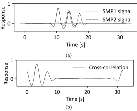
reasonable for road bridges, where the mass of the vehicle is typically less than about
82
4% of the mass of the bridge. For railway bridges the mass of the train may be 10% or
83
more of the bridge mass. The influence of the large mass of a train on the dynamic
84
behaviour of the system may cause inaccuracies in the calculated weights using
85
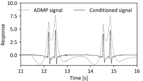
standard B-WIM methods. It may be necessary to develop new, more sophisticated
86
algorithms which allow for the influence of the train mass/bridge mass dynamic
87
interaction.
88
• Trains have many more axles than trucks – trains consist of numerous axles which are
89
generally in groups of 2 or 3. Many closely spaced axles can lead to ill-conditioning of
90
the equations used in conventional B-WIM systems.
91
• Axle detection may be more difficult for railway bridges – train axles can easily be
92
identified by instrumenting the rails. However, it is not always feasible to instrument
93
the rail, specifically on busy lines where rail closure is not an option, or where the use
94
of electrical resistance gauges is infeasible on electrified systems. Where the rail cannot
95
be instrumented, it may be difficult to identify individual axles within groups, especially
96
for ballasted tracks where the axle forces are distributed through the sleepers and the
97
ballast and measured signals do not show peaks for individual axles.
98
• In the light of the difficult and possibly erroneous axle detection, a general algorithm for
99
rolling stock identification would be very complex. The issue is further complicated by
100
the presence of Jacobs bogies, commonly found on articulated railcars.
101
Building on lessons learned in developing road B-WIM, this paper describes the development
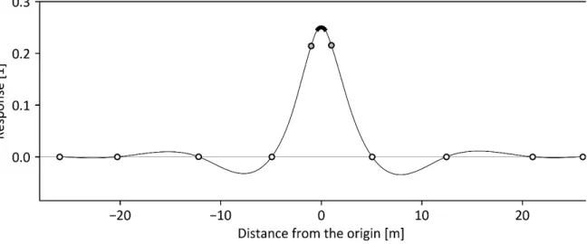
102
and testing of a new railway bridge WIM system (RB-WIM). RB-WIM provides a better
103
understanding of railway traffic loads and consequently their effects on railway bridges. This system
104
was developed as part of BridgeMon, a 2-year research project funded under the European
105
Commission’s 7th Framework programme. A steel truss bridge at Nieporęt in Poland was used as a
106
case study and to test the accuracy of the system.
107
2. RB-WIM Algorithm
108
Most operational B-WIM algorithms work on the assumption of static conditions, similar to that
109
proposed by Moses [21]. This is built upon the observation that, during the passage of a truck, the
110
bridge oscillates about a static response. Assuming strain transducers attached to each bridge beam
111
or strip of a slab at G measurement points, the average measured strain at time, t, 𝜀𝜀̅(𝑡𝑡), can be found
112
by averaging the individual values:
113
𝜀𝜀̅
(
𝑡𝑡
𝑗𝑗) =
𝐺𝐺 � 𝜀𝜀
1
𝑖𝑖(
𝑡𝑡
)
𝐺𝐺 𝑖𝑖=
𝐶𝐶
𝐹𝐹� 𝜀𝜀
𝑖𝑖(
𝑡𝑡
)
𝐺𝐺 𝑖𝑖 (1) where εi(𝑡𝑡) is the strain in the ithgirder or section of slab at time t, and CF is a calibration factor.114
The calibration factor CF can also incorporate strain transducer factors relating strain to voltage and
115
is obtained experimentally by correlating the B-WIM results for some vehicles with their true axle
116
loads, as measured on static scales.
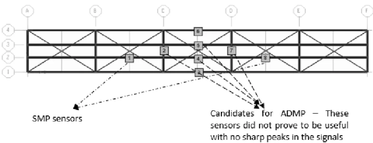
117
In the B-WIM algorithm, the number of unknowns for each vehicle is equal to the number of
118
axles, N, and these are determined by at least N different measurements recorded for different
119
longitudinal positions of the vehicle along the bridge. Setting up the equations requires the strain
120
influence lines, I(x). The procedures to calculate a bridge influence line based on measurements are
121
described in section 2.2. Taking the origin at the peak of the influence line and letting the first axle
122
arrive at this point at time zero, the first axle is at, x = vt at time, t, where v is velocity. Hence, the ith
123
axle is at x = v(t – ti) at time, t, where ti is the time interval between the arrivals of the 1st and ith axles.
124
The B-WIM weighing challenge is then to minimise the sum of squares of differences between the
125
measured strains of Eq. 1 and the theoretical equivalents, given as the sum of contributions from each
126
axle:127
min� �𝜀𝜀̅(𝑡𝑡)− � 𝐴𝐴𝑖𝑖𝐼𝐼[v(𝑡𝑡 − 𝑡𝑡𝑖𝑖)] 𝑁𝑁 𝑖𝑖=1 � 2 (2) where summation is overthe number of scans (each corresponding to a different point in time),128
Ai is the weight of axle i, N is the number of axles and I(x) is the influence line value. With a scan rate
129
of 512 samples per second and vehicle passage duration of the order of seconds, the number of
130
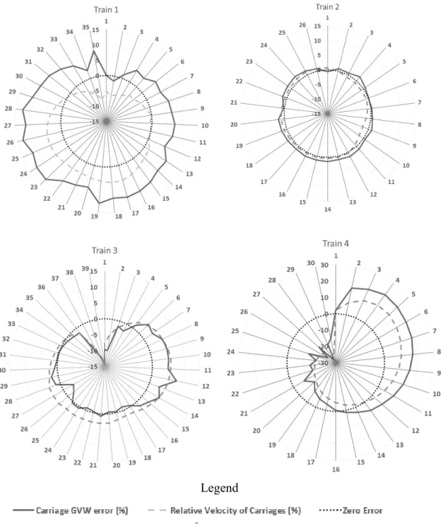
equations is typically one or two orders of magnitude greater than the number of unknowns. This
131
over-determined system of equations is solved for Ai, in the least-square sense, with the use of the
132
singular value decomposition algorithm [33].
133
2.1. Train Velocity and Axle Determination
134
Commercial B-WIM for road vehicles breaks the continuous strain signal into segments of data
135
known as bridge loading ‘events’. The settings for the splitting algorithm are chosen so that the
136
segments contain enough data to ensure that the influence of the vehicles within each event do not
137
extend beyond event boundaries. The weighing algorithm uses these events as basic units of
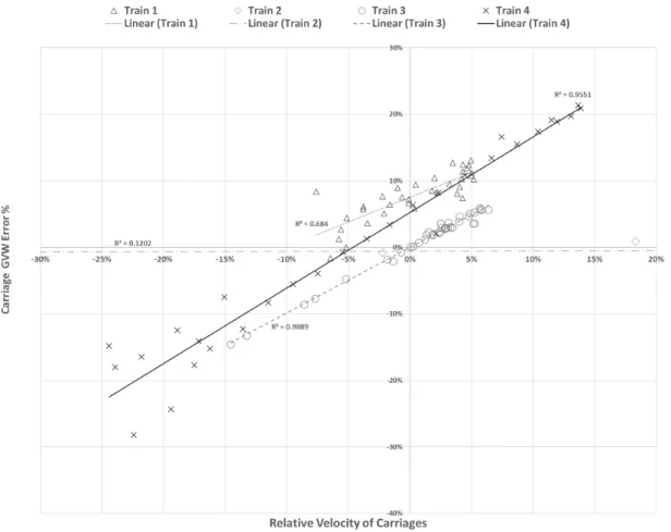
138
information.
139
In addition to the signals from the strain transducers, two additional classes of signal need to be
140
acquired in order to solve the system of equations: signals from which the axles are detected and the
141
vehicle velocity is computed. The requirements for these classes of signals are different.
142
Calculating the vehicle velocity requires at least two sensors mounted at so-called Speed
143
Measurement Points (SMPs), which need to be located at different longitudinal locations along the
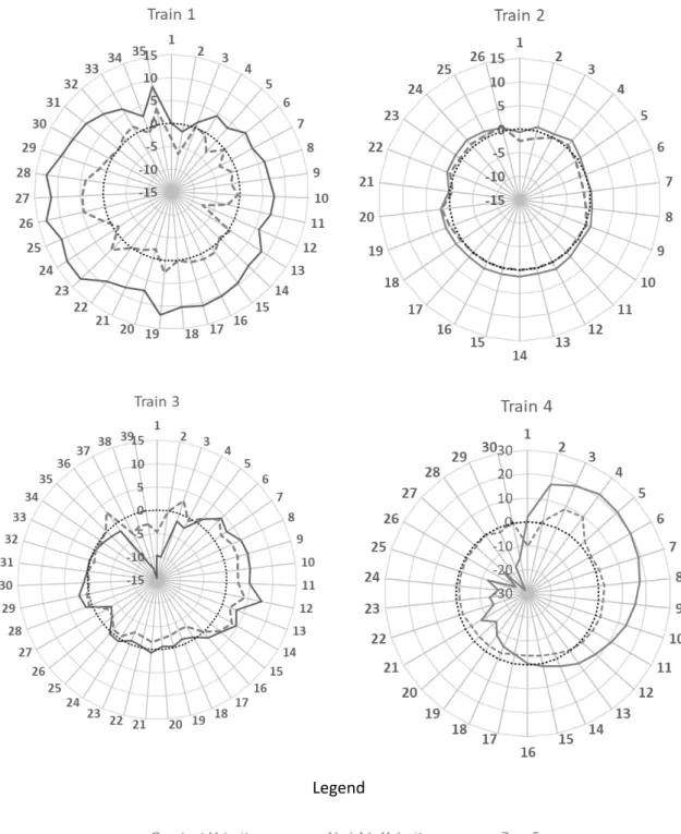
144
bridge. The exact shapes of these signals are not crucial, as long as the vehicle can be clearly identified
145
in the signals. While sharper and more symmetrical peaks will give better speed accuracy, relatively
146
smooth signals have been found to be sufficient.
147
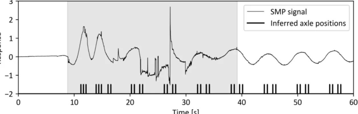
In contrast to SMPs, sensors located at the Axle Detection Measurement Points (ADMPs) need
148
to have pronounced peaks in order to accurately determine the axle positions. It is possible to use
149
advanced filtering and vehicle reconstruction algorithms to partially mitigate this [34], but it is much
150
better to start with good signals. Depending on the details of the installation, a sensor may play more
151
than one role. For example, on a typical road installation, one of the SMPs may be used as an ADMP.
152
In the case of the tested railway bridge in Poland, a separate sensor, dedicated to axle detection,
153
needed to be installed, as explained below.
154
The correlation between two signals from SMPs defines the time shift of one signal relative to
155
the other and hence is used to find the speed. An example for a one-carriage passenger train is
156
presented in Figure 1. The solid and dashed traces of Figure 1(a) represent the signals measured at
157
the first and the second SMP, respectively; Figure 1(b) shows the correlation. The location of the peak
158
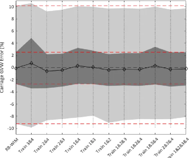
in the correlation is used to determine the time shift, 2.475 s in this case. The calculated time shift and
159
the known distance between the SMPs are used to determine the speed of the vehicle.
160
(a)
(b)
Figure 1. An example of correlation of SMPs for a one-carriage passenger train: a. SMP for two signals
161
b. Cross-correlation of the two signals
162
Once the vehicle speed is known, the axles of a train are detected using the same algorithm used
163
for road bridges [34]. The signal from the sensor is conditioned by applying two moving average
164
filters with different averaging lengths. The moving average with the shorter length is used to smooth
165
out the high-frequency noise; the other is used to determine the general shape of the response. The
166
two filtered signals are subtracted and the resulting difference is examined to identify all peaks above
167
a specified threshold level. These peaks correspond to the passing of individual axles. Figure 2 shows
168
the axle detection signal and the conditioned signal for a one-carriage passenger train. The
169
conditioned signals can be seen to have clear peaks corresponding to the four passing axles.
170
Figure 2. Raw ADMP signal and conditioned signal for a one-carriage passenger train
171
Once the speed of the vehicle and the times of passage of individual axles have been obtained,
172
the intra- and inter-bogie spacings are calculated.
173
2.2.Influence lines
174
Influence lines (IL) are key properties of a bridge, defining how it responds to loading at a given
175
measurement point [24]. It has been shown that influence lines should be calculated directly from
176
measurements [35] since theoretical influence lines rarely provide an accurate description of bridge
177
behaviour. Two methods of ‘measuring’ influence lines for bridges are known, the SiWIM approach
178
[34] and the Matrix Method [36]. The Matrix Method uses vehicles of known axle loads and spacings
179
and an inverse Moses algorithm to derive the experimental influence lines. This method is more
180
straightforward and less time-consuming but requires vehicles of known weight, which are not
181
always available at the time of setting-up the B-WIM system. More recently, a variation on this
182
approach addresses the issue of requiring a vehicle of known weight [37].
183
The SiWIM system, used here, calculates the influence lines for the bridge using selected vehicles
184
with unknown axle loads. Numerous evaluations of influence lines can be averaged to improve
185
accuracy. Such IL’s are normalised and require a scalar calibration factor to convert relative axle
186
weights to actual weights (the CF parameter in Equation 1). A detailed explanation of this general
187
procedure of IL calculation can be found in [34]. Briefly, the system models the IL with a cubic spline,
188
chosen because its general characteristics match well with real influence lines – it is a curve of third
189
order, continuous and smooth in first and second derivatives [33]. Some of the spline knots,
190
representing supports and endpoints, are fixed, while some are allowed to vary. In order to determine
191
the values and thus the shape of the IL, Equation 2 is used. Contrary to its use in weighing, where
192
the only unknowns are axle loads, Ai, the function, I(x) is unknown when calculating the IL. Since the
193
system is no longer a linear function of all unknowns, Powell’s minimisation [33] is used to solve the
194
problem.
195
Figure 3 shows the IL calculated for the Nieporęt Bridge, for sensors mounted at the base of the
196
truss at mid-span. The white points represent the fixed knots, while the ordinates of the two grey
197
points were varied in order to obtain the best fit. For this bridge, local bending of the stringer beams
198
dominated over global truss bending, making the influence line similar to that for a continuous beam
199
with supports at truss chord locations. This effect was accentuated by setting the fixed knots to zero
200
at the chord locations (Figure 3).
201
Figure 3.Influence line for the Nieporęt Bridge
202
A theoretical influence line for an infinitely thin bridge (Euler Bernoulli beam) has a sharp peak
203
at mid-span where the derivative is discontinuous. In contrast, the peak of the influence line for a real
204
bridge has a rounded peak, which is approximated by a circular portion, whose radius corresponds
205
roughly to the superstructure thickness. This peaked section is drawn in bold in Figure 3 and the
206
radius was also varied to obtain the best fit.
207
3. RB-WIM Installation and Testing
208
A typical truss bridge in Poland was selected for testing of the RB-WIM system (Figure 4). The
209
bridge is located in Nieporęt, near Warsaw. Constructed in the 1970’s, it is one of over one thousand
210
similar bridges in Poland [38]. It spans 40 m and consists of five 8 m long bays. The bridge has
211
deteriorated significantly since first constructed. As a result, the velocity of the crossing trains is
212
limited to 20 km/h [39].
213
(a) (b)
Figure 4. Nieporęt Bridge: (a) elevation and (b) view from underneath
214
The bridge is supported on four steel bearings, illustrated in Figure 5, two at each end. It carries
215
a single unballasted railway track which runs along the centre. The structure of the bridge consists of
216
two main vertical trusses, one at either side. The trusses are connected along the bottom by six cross
217
beams which are located at the node points of the bottom chord.
218
The railway track is supported by timber sleepers which span onto two ‘stringer’ beams. These
219
stringer beams extend longitudinally and are supported by the six cross beams. The loading on the
220
track is transferred onto the sleepers and then onto the stringer beams. The stringer beams transfer
221
the load into the cross beams which are supported at the node points of the trusses.
222
(a)
(b)
Figure 5. Nieporęt Bridge: steel bearings
223
The Nieporęt Bridge has been studied since mid-2007 due to interest from Polish Railways in
224
the development of Structural Health Monitoring (SHM) systems for railway bridges [40]. The bridge
225
has been instrumented with a number of sensors, data from which are in the literature [40]. Prior to
226
installation of the RB-WIM system, some of these published results were used to confirm the accuracy
227
of the static model. For this purpose a finite element model of the bridge was created using the Midas
228
finite element software package. The bridge was modelled using beam elements, with full fixity
229
assumed at node points. The design drawings were used to calculate cross sectional properties. A
230
Young’s Modulus of E = 210×106 kN/m2 was assumed throughout [41]. Figure 6 shows the MIDAS
231
model of the bridge, identifying some of the main structural elements. The rail and sleepers have
232
been omitted for clarity. The numerical model of the bridge was validated at a number of important
233
measurement locations using recordings from a previous measurement campaign [40]. Having
234
established a good match between the response of the model and the measurements collected by
235
Kołakowski et al. [40], it was used to develop the instrumentation strategy for the in-field testing of
236
the RB-WIM concept.
237
Figure 6. MIDAS Model of Nieporęt Bridge [41]
238
Strain transducers were installed on the longitudinal trusses, on the stringers and on the cross
239
beams, to provide full coverage in the central part of the truss. Sensors were also located on one
240
stringer beam in the bays either side of the centre (i.e. sensors 1 and 8 shown in Figure 7). The
241
locations of the sensors are marked with grey squares on Figure 7. The numbers represent the data
242
acquisition channels. To avoid welding or drilling, steel mounting plates were used as interfaces.
243
They were bonded to the structure with epoxy and, after hardening, the strain sensors were fastened
244
with nuts. Additionally, strain gauges were bonded directly to the bridge at locations 3 through 6.
245
Figure 7. Sensor locations (plan view of bridge at track level)
246
A desirable characteristic of a B-WIM installation is that any intervention on the track side is
247
avoided, an important advantage from a safety and maintenance perspective. Therefore, it was
248
envisaged that the sensors on the stringer beams, right under the sleepers, would be used for axle
249
detection. However, signals from the passing trains revealed that the axle loads distributed over the
250
entire rail-sleeper-bridge system did not provide sharp peaks to identify individual axles in a bogie
251
(double or triple axles – Figure 8). Thus, the sensors were moved from their initial locations to the
252
bottom flange of the rail between two sleepers.
253
Figure 8. Signals collected from the stringers beams and ADMP
254
Field testing was performed between May 20th and 25th, 2013. Over the first two days, the sensors
255
and the system were installed. On May 22nd, the first of four calibration/test trains, which were
256
weighed off-site, passed the bridge. Signals from three other pre-weighed trains were also captured;
257
two on May 24th and one on 25th.
258
The four calibration/test trains were weighed on a low-speed weigh-in-motion scale in a railway
259
yard in Warsaw that operates at speeds of up to 5 km/h. All of these trains consisted of a 6-axle
260
locomotive and 25 to 38 carriages of different length, axle configuration and loading. Due to the
261
limitations of the low-speed device, only gross weights of carriages, without individual axle loads,
262
were available for comparison with the B-WIM results.
263
4. Results and Discussion
264
Figure 9 summarises the initial results for all four pre-weighed trains in a spider chart. The solid
265
black line represents the error in GVW estimated using the RB-WIM algorithm applied to the 35
266
locomotives/individual carriages. The dashed grey line represents the relative velocity of individual
267
carriages, calculated as the ratio of the individual carriage velocity to the average velocity of the entire
268
train, as described in section 3.1. While the train speed can be assumed to be constant at any point in
269
time, it varies through time. The speed limit on the bridge was 20 km/h. It appears that this was not
270
adhered to precisely by the drivers, but its presence resulted in significant braking and acceleration
271
as the trains crossed.
272
It can be seen that the carriage accuracy for Train 2 represents the best match with maximum
273
weight error of 2% and standard deviation of 0.64%. The maximum error in GVW estimation occurs
274
in Train 4 with error of up to 28%. The obvious reason for this error is the assumption of constant
275
velocity for all carriages in an event where it is varying quite significantly about the mean. The
276
assumption of constant velocity is reasonable on roads, as trucks typically cross a short-span bridge
277
in one or two seconds, but trains are too long for such an assumption.
278
Legend
Figure 9. Error in GVW of carriages and relative velocity of individual carriages – Train 1-4
279
The speed variation was more pronounced for longer trains, some of which exceeded 500 m in
280
length. As the variation in measured speed in the worst case (Train 4) surpassed 25% (negative error),
281
the assumption of constant velocity clearly was not appropriate and had to be addressed. Figure 10
282
shows the correlation between the error in carriage GVW and the relative velocity for all carriages of
283
all four trains. It can be seen that Train 3 and 4 in particular show strong linear correlations between
284
GVW error and relative velocity with correlation coefficients of 0.99 and .96 respectively.
285
Figure 10. Correlation between Carriage GVW error and Relative Velocity of Carriages
286
To address this issue, the constant velocity of the whole train is replaced with different velocities
287
for individual carriages. The additional step in the modified algorithm consists of determining the
288
sections of the SMP signals where a locomotive/carriage is on the bridge (as isolated as possible),
289
calculating the correlations for only those parts of the signals and assigning the resulting speeds to
290
the locomotive/carriage in question.
291
Figure 11 displays the errors in the predicted carriage gross weights for each train when
292
considering (i) the average velocity of the train obtained from the entire train crossing (solid black
293
line curves as shown in Figure 9) and (ii) variable velocities calculated for each carriage (dashed grey
294
line). There are clear improvements in accuracy for all four trains. The improvements are less
295
pronounced for Trains 2 and 3 but the accuracy for these was already good and it is significant that,
296
where there were some larger errors in Train 3 (Carriages 37-39), these are greatly reduced. The
297
improvements in Train 4 are quite pronounced although some errors persist at Carriages 1, 3 and 4.
298
This may be explained by the occurrence of heavy rain just before the crossing of this train and
299
insufficient protection of the strain gauges (due to the short testing campaign) which resulted in a
300
noisy speed measurement signal (the shaded area in Figure 12) and, consequently, unreliable velocity
301
measurements for these carriages. Such errors can easily be avoided in the future by protecting the
302
sensors against environmental effects.
303
Legend
Figure 11. Error in gross weights of carriages (i) when train is assumed to have constant velocity
304
and (ii) when carriage velocities are calculated separately – Trains 1 to 4
Figure 12. Noise in speed measurement signals
306
Figure 13 summarises the results obtained with the original RB-WIM algorithm and those
307
obtained using the revised algorithm for all four reference trains (calibration trains). It can be seen
308
from this figure that the mean error in GVW is considerably reduced by the revised algorithm. For
309
Train 4 in particular, the maximum error is reduced from 28.19 to 10.17%. The weights of the Train 2
310
carriages were predicted very accurately which can be linked to constant travelling speed and
311
uniform distribution of carriage weights.
312
a.
Mean error
b.
Coefficient of variation
Figure 13. Comparison between Original and Revised Algorithm313
In the results up to this point, all four trains were used to calibrate the system. As such, the mean
314
weight is not an indication of the accuracy but the low standard deviation indicates an excellent level
315
of accuracy relative to conventional road weigh-in-motion technologies. To investigate the sensitivity
316
of the algorithm to the chosen calibration/test trains, 11 permutations of the calibration database are
317
considered using all possible combinations of the four trains for calibration. These combinations are
318
then used to produce a linear regression model between predicted GVW using the revised RB-WIM
319
algorithm and the measured GVWs of carriages. Using each regression model, the GVWs of carriages
320
and locomotives for each train are calculated and compared to the corresponding static values (Figure
321
14). The light grey area in this figure shows the minimum and maximum range of errors for each
322
regression model and the dark grey represents the mean of the errors in carriage GVW ± one standard
323
deviation (for each model). The horizontal dashed lines represent the minimum, maximum and mean
324
± one standard deviation. It can be seen that there is little difference in the results except for
325
calibration using Trains 3 & 4, likely due to the poor accuracy of Train 4.
326
Figure 14. Carriage GVW error for the regression models with different dataset and the revised
327
algorithm considering variable carriage velocity
328
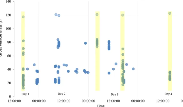
According to the railway authorities in Poland, there is a very common 120 tonne locomotive
329
that operates on the network. At the time of the measurements for this study, in addition to the four
330
calibration trains, another two trains with locomotives of approximate 120 tonne gross vehicle mass
331
were measured. In this figure, each point represents an individual locomotive/carriage and points
332
aligned in the vertical direction (with small timestamp difference) represent one train. Figure 15
333
presents all measured trains and time of measurement. Both in the trains with 120 t locomotives and
334
others, there are carriages/locomotives weighing about 80 t with most of the remaining carriages
335
ranging between 20 t and 50 t.
336
Figure 15. Gross Vehicle Mass of measured locomotives and carriages for four days of measurement
337
Figure 16a illustrates a particular train with 40 carriages where it can be seen that the front
338
carriages are much more heavily loaded than the others. Figures 16 b and c provide a closer view of
339
two groups of carriages 2-23 and carriages 24-40, respectively. Apart from the locomotive, the front
340
carriages all have weights between 74 and 81 t. There is a dramatic drop at Carriage 24 and all
341
remaining carriages weigh between 20 t and 28 t.
342
Figure 16. Gross Vehicle Mass Estimation for an uncalibrated train
344
5. Conclusions
345
Knowing the true weights of trains is becoming more important, particularly in Europe due to
346
the splitting of the operation and infrastructure maintenance roles of the relevant authorities. This
347
paper adapted a commercial road B-WIM system for use on railways. An old railway bridge in
348
Nieporęt in Poland was used to test the accuracy of the new RB-WIM system.
349
Initial results demonstrated that one of four pre-weighed trains, the only one which crossed the
350
bridge at constant speed, was weighed very accurately, with all carriage weight errors falling within
351
the -0.9% to 1.6% error interval. Disappointing levels of accuracy for the other pre-weighed trains
352
was shown to be the result of variable carriage speed in the time that the train took to cross the bridge.
353
Results improved significantly when this was addressed, with 75% of all calculated carriage weights
354
falling within ±2% and 97% of them falling within ±5% of their actual values. These values include 4
355
carriages which had an issue with axle detection due to rain.
356
6. Acknowledgments
357
Funding: This work was supported through the BridgeMon project. BridgeMon was funded by the European
358
Commission 7th Framework Programme (grant agreement n°315629).
359
Acknowledgments: The authors also gratefully acknowledge the contributions of the other BridgeMon
360
consortium partners: CESTEL CESTNI INZENIRING DOO and ADAPTRONICA ZOO SP.
361
a. All carriages
References
362
1. Filograno, M.L.; Rodríguez-Barrios, A.; González-Herraez, M.; Corredera, P.; Martín-López, S. Real time
363
monitoring of railway traffic using fiber bragg grating sensors. Proc. 2010 Jt. Rail Conf. 2010, 1–8.
364
2. Minardo, A.; Porcaro, G.; Giannetta, D.; Bernini, R.; Zeni, L. Real-time monitoring of railway traffic using
365
slope-assisted Brillouin distributed sensors. Appl. Opt. 2013, 52, 3770, doi:10.1364/AO.52.003770.
366
3. Carvalho Neto, J.A. DE; Veloso, L.A.C.M. Weighing in motion and characterization of the railroad traffic
367
with using the B-WIM technique. Rev. IBRACON Estruturas e Mater. 2015, 8, 491–506,
doi:10.1590/S1983-368
41952015000400005.
369
4. Marques, F.; Moutinho, C.; Hu, W.H.; Cunha, A.; Caetano, E. Weigh-in-motion implementation in an
370
old metallic railway bridge. Eng. Struct. 2016, 123, 15–29, doi:10.1016/j.engstruct.2016.05.016.
371
5. Alampalli, S. Special Issue on Nondestructive Evaluation and Testing for Bridge Inspection and
372
Evaluation. J. Bridg. Eng. 2012, 17, 827–828, doi:10.1061/(ASCE)BE.1943-5592.0000430.
373
6. Cross, E.J.; Koo, K.Y.; Brownjohn, J.M.W.; Worden, K. Long-term monitoring and data analysis of the
374
Tamar Bridge. Mech. Syst. Signal Process. 2013, 35, 16–34, doi:10.1016/j.ymssp.2012.08.026.
375
7. Chellini, G.; Lippi, F.V.; Salvatore, W. A multidisciplinary approach for fatigue assessment of a steel–
376
concrete high-speed railway bridge on Sesia river. Struct. Infrastruct. Eng. 2014, 10, 189–212,
377
doi:10.1080/15732479.2012.719527.
378
8. Dudás, K.; Jakab, G.; Kövesdi, B.; Dunai, L. Assessment of Fatigue Behaviour of Orthotropic Steel Bridge
379
Decks using Monitoring System. Procedia Eng. 2015, 133, 770–777, doi:10.1016/j.proeng.2015.12.660.
380
9. Farreras-Alcover, I.; Chryssanthopoulos, M.K.; Andersen, J.E. Data-based Models for Fatigue Reliability
381
of Orthotropic Steel Bridge Decks based on Temperature, Traffic and Strain Monitoring. Int. J. Fatigue
382
2016, doi:10.1016/j.ijfatigue.2016.09.019.
383
10. Saberi, M.R.; Rahai, A.R.; Sanayei, M.; Vogel, R.M. Bridge Fatigue Service-Life Estimation Using
384
Operational Strain Measurements. J. Bridg. Eng. Am. Soc. Civ. Eng. 2016, 04016005,
385
doi:10.1061/(ASCE)BE.1943-5592.0000860.
386
11. Cheung, M.S.; Tadros, G.S.; Brown, T.; Dilger, W.H.; Ghali, A.; Lau, D.T. Field monitoring and research
387
on performance of the Confederation Bridge. Can. J. Civ. Eng. 1997, 24, 951–962, doi:10.1139/l97-081.
388
12. Mufti, A.A. Structural Health Monitoring of Innovative Canadian Civil Engineering Structures. Struct.
389
Heal. Monit. 2002, 1, 89–103, doi:10.1177/147592170200100106.
390
13. Desjardins, S.L.; Londoño, N.A.; Lau, D.T.; Khoo, H. Real-Time Data Processing, Analysis and
391
Visualization for Structural Monitoring of the Confederation Bridge. Adv. Struct. Eng. 2006, 9, 141–157,
392
doi:10.1260/136943306776232864.
393
14. Ghodoosipoor, F. Development of Deterioration Models for Bridge Decks Using System Reliability
394
Analysis, Concordia University, Montréal, Québec, Canada, 2013.
395
15. Clarke, J.N. Investigating the Remaining Fatigue Reliability of an Aging Orthotropis Steel Plate Deck,
396
Dalhousie University, 2014.
397
16. Watanabe, E.; Furuta, H.; Yamaguchi, T.; Kano, M. On longevity and monitoring technologies of bridges:
398
a survey study by the Japanese Society of Steel Construction. Struct. Infrastruct. Eng. 2014, 10, 471–491,
399
doi:10.1080/15732479.2013.769008.
400
17. Sakagami, T. Remote nondestructive evaluation technique using infrared thermography for fatigue
401
cracks in steel bridges. Fatigue Fract. Eng. Mater. Struct. 2015, 38, 755–779, doi:10.1111/ffe.12302.
402
18. Yan, F.; Chen, W.; Lin, Z. Prediction of fatigue life of welded details in cable-stayed orthotropic steel
403
deck bridges. Eng. Struct. 2016, 127, 344–358, doi:10.1016/j.engstruct.2016.08.055.
19. Guo Tong, T.; Li Aiqun, A.; Li Jianhui, J. Fatigue Life Prediction of Welded Joints in Orthotropic Steel
405
Decks Considering Temperature Effect and Increasing Traffic Flow. Struct. Heal. Monit. 2008, 7, 189–202,
406
doi:10.1177/1475921708090556.
407
20. Inaudi, D. Overview of 40 Bridge Structural Health Monitoring Projects. In Proceedings of the
408
International Bridge Conference, IBC 09-45; 2010.
409
21. Moses, F. Weigh-in-motion system using instrumented bridges. J. Transp. Eng. 1979, 105.
410
22. COST323 Weigh-in-Motion of Road Vehicles: Final Report of the COST 323 Action; 2002;
411
23. WAVE Bridge WIM. Report of Work Package 1.2.; 2001;
412
24. OBrien, E.J.; Znidaric, A.; Ojio, T. Bridge weigh-in-motion—Latest developments and applications world
413
wide. In Proceedings of the Proceedings of the International Conference on Heavy Vehicles; 2008; pp.
414
19–22.
415
25. Richardson, J.; Jones, S.; Brown, A.; O’Brien, E.; Hajializadeh, D. On the use of bridge weigh-in-motion
416
for overweight truck enforcement. Int. J. Heavy Veh. Syst. 2014, 21, 83–104.
417
26. Liljencrantz, A.; Karoumi, R.; Olofsson, P. Implementation of bridge weigh-in-motion for railway traffic.
418
In Proceedings of the Fourth international conference on weigh-in-motion; 2005.
419
27. Liljencrantz, A.; Karoumi, R. Twim: A MATLAB toolbox for real-time evaluation and monitoring of
420
traffic loads on railway bridges. Struct. Infrastruct. Eng. 2009, 5, 407–417, doi:10.1080/15732470701478370.
421
28. Liljencrantz, A.; Karoumi, R.; Olofsson, P. Implementing bridge weigh-in-motion for railway traffic.
422
Comput. Struct. 2007, 85, 80–88, doi:10.1016/j.compstruc.2006.08.056.
423
29. Gonzalez, I.; Karoumi, R. Traffic monitoring using a structural health monitoring system. ICE Proc. 2015,
424
168, 13–23, doi:http://dx.doi.org/10.1680/bren.11.00046.
425
30. Quilligan, M. Bridge Weigh-in-Motion: development of a 2-D multi-vehicle algorithm. Trita-BKN. Bull.
426
2003, 69, A--144.
427
31. González, A.; Rowley, C.; OBrien, E.J. A general solution to the identification of moving vehicle forces
428
on a bridge. Int. J. Numer. Methods Eng. 2008, 75, 335–354.
429
32. Rowley, C.W.; OBrien, E.J.; González, A.; Žnidarič, A. Experimental testing of a moving force
430
identification bridge weigh-in-motion algorithm. Exp. Mech. 2009, 49, 743–746.
431
33. Press, W.H.; Teukolsky, S.A.; Vetterling, W.T.; Flannery, B.P. Numerical recipes: the art of scientific
432
computing; 3rd Editio.; Cambridge University Press, 2007;
433
34. Žnidarič, A.; Kalin, J.; Kreslin, M. Improved accuracy and robustness of bridge weigh-in-motion
434
systems. Struct. Infrastruct. Eng. 2017, 2479, 412–424, doi:10.1080/15732479.2017.1406958.
435
35. Znidaric, A.; Lavric, I.; Kalin, J. The next generation of bridge weigh-in-motion systems. In Proceedings
436
of the Third International Conference on Weigh-in-Motion (ICWIM3); 2002.
437
36. OBrien, E.J.; Quilligan, M.; Karoumi, R. Calculating an influence line from direct measurements. Proc.
438
Inst. Civ. Eng. Eng. 2006, 159, 31–34.
439
37. OBrien, E.J.; Schoefs, F.; Heitner, B.; Causse, G.; Yalamas, T. Finding the influence line for a bridge based
440
on random traffic and field measurements on site. In Proceedings of the Civil Engineering Research in
441
Ireland 2018, Eds. V. Pakrashi & J. Keenahan, Civil Engineering Research Association of Ireland
442
(CERAI), Dublin, 28-30 Aug., 790-794.; 2018.
443
38. Kołakowski, P.; Szelążek, J.; Sekuła, K.; Świercz, A.; Mizerski, K.; Gutkiewicz, P. Structural health
444
monitoring of a railway truss bridge using vibration-based and ultrasonic methods. Smart Mater. Struct.
445
2011, 20, 035016, doi:10.1088/0964-1726/20/3/035016.
446
39. Žnidarič, A.; Kalin, J.; Kreslin, M.; Favai, P.; Kolakowski, P. Railway Bridge Weigh-in-Motion System.
Transp. Res. Procedia 2016, 14, 4010–4019.
448
40. Kołakowski, P.; Sala, D.; Pawłowski, P.; Swiercz, A.; Sekuła, K. Implementation of SHM system for a
449
railway truss brigde. 2011.
450
41. Favai, P.; OBrien, E.; Žnidarič, A.; Van Loo, H.; Kolakowski, P.; Corbally, R. Bridgemon : Improved
451
monitoring techniques for bridges. In Proceedings of the Civil Engineering Research in Ireland, Belfast,
452
UK, 28- 29 August, 2014; 2014.
453
454
© 2020 by the authors. Submitted for possible open access publication under the terms and conditions of the Creative Commons Attribution (CC BY) license (http://creativecommons.org/licenses/by/4.0/).