Lunn, David; Barrett, Jessica; Sweeting, Michael; Thompson, Si-mon (2013) Fully Bayesian hierarchical modelling in two stages, with application to meta-analysis. JOURNAL OF THE ROYAL STATIS-TICAL SOCIETY SERIES C-APPLIED STATISTICS, 62 (4). pp. 551-572. ISSN 0035-9254 DOI: https://doi.org/10.1111/rssc.12007 Downloaded from: http://researchonline.lshtm.ac.uk/4652043/
DOI:10.1111/rssc.12007
Usage Guidelines
Please refer to usage guidelines at http://researchonline.lshtm.ac.uk/policies.html or alterna-tively [email protected].
©2013 Royal Statistical Society 0035–9254/13/62551 62,Part4,pp.551–572
Fully Bayesian hierarchical modelling in two stages,
with application to meta-analysis
David Lunn, Jessica Barrett, Michael Sweeting and Simon Thompson Medical Research Council Biostatistics Unit, Cambridge, UK
[Received February 2012. Final revision November 2012]
Summary.Meta-analysis is often undertaken in two stages, with each study analysed separately in stage 1 and estimates combined across studies in stage 2. The study-specific estimates are assumed to arise from normal distributions with known variances equal to their corresponding estimates. In contrast, a one-stage analysis estimates all parameters simultaneously. ABayesian
one-stage approach offers additional advantages, such as the acknowledgement of uncertainty in all parameters and greater flexibility. However, there are situations when a two-stage strategy is compelling, e.g. when study-specific analyses are complex and/or time consuming.We present a novel method for fitting the full Bayesian model in two stages, hence benefiting from its advanta-ges while retaining the convenience and flexibility of a two-stage approach. Using Markov chain Monte Carlo methods, posteriors for the parameters of interest are derived separately for each study. These are then used as proposal distributions in a computationally efficient second stage. We illustrate these ideas on a small binomial data set; we also analyse motivating data on the growth and rupture of abdominal aortic aneurysms. The two-stage Bayesian approach closely reproduces a one-stage analysis when it can be undertaken, but can also be easily carried out when a one-stage approach is difficult or impossible.
Keywords: Abdominal aortic aneurysm; Bayesian hierarchical modelling; BUGS; Markov
chain Monte Carlo methods; Random-effects meta-analysis
1. Introduction
1.1. Standard methods of meta-analysis and their limitations
Meta-analysis is often undertaken in two stages, even when individual participant data are available. At the first stage, each study is analysed to provide an estimate of the parameter of interest, together with its standard error. At the second stage, the estimates are combined across studies; in a random-effects meta-analysis, potential heterogeneity between the study-specific
parameters is permitted (Higginset al., 2009).
Writingxi as the estimate of parameterθi in studyi, with the standard error denoted bysi,
the usual two-stage random-effects meta-analysis model is xi∼N.θi,s2i/
within each studyi, and
θi∼N.μ,σ2/
across studiesi=1, . . . ,N, whereσ2is the between-study heterogeneity variance. In practice,s2i
Address for correspondence: David Lunn, Medical Research Council Biostatistics Unit, Institute of Public Health, University Forvie Site, Robinson Way, Cambridge, CB2 0SR, UK.
E-mail: [email protected]
Reuse of this article is permitted in accordance with the terms and conditions set out at http://wiley onlinelibrary.com/onlineopen#OnlineOpen Terms.
is estimated but then assumed to be without error in the above model, and normal distributions are assumed at both the first and the second stages. Although estimation of the overall
parame-tersμandσ2can be by maximum likelihood or restricted maximum likelihood, a (non-iterative)
moment estimator ofσ2is most often used in practice. The inference aboutμis usually made
by using an asymptotic normal approximation (i.e. asymptotic with respect to the number of
studies), assuming thatσ2is fixed and known.
A Bayesian version of this model, in which study-specific and overall parameters are estimated simultaneously, can be implemented straightforwardly by using Markov chain Monte Carlo
(MCMC) methods (Gelfand and Smith, 1990; Metropoliset al., 1953; Hastings, 1970). This
has several advantages: for example, uncertainty on all parameters, includingσ2, is
acknowl-edged simultaneously, prior information may be incorporated (e.g. Smithet al.(1995)), a credible
interval forμcan simply be taken from the quantiles of its estimated posterior distribution, with
no asymptotic normal approximation needed, and although the normality assumption for the between-study model is usually retained, a more flexible distribution could be used in principle (Lee and Thompson, 2008).
The focus of this paper, however, is on exploiting individual participant data, where available, to avoid the need for two potentially limiting assumptions in the above model:
(a) that the study-specific estimates are normally distributed; (b) that the associated uncertainties (variances) are known.
The former may be inappropriate for studies with relatively sparse data, or when the parame-ters of interest are unconventional. The latter is circumvented with individual participant data because the full uncertainty regarding study-specific parameters is naturally propagated into the between-study model, and feedback is allowed from the between-study model to the esti-mation of study-specific parameters. For simple data structures, a non-Bayesian analysis can be achieved by using linear mixed models for continuous outcomes, or generalized linear mixed
models for binary outcomes. The inference aboutμ, however, is again usually made by using an
asymptotic normal approximation, assuming thatσ2is fixed and known (Higginset al., 2001).
Alternatively, a Bayesian analysis can be implemented using MCMC sampling. In addition to the advantages that were outlined above, MCMC methods can be used when the study-specific data structures are complex.
Meta-analyses that make use of individual participant data are currently less common than their aggregate data counterparts, but their application is on the rise, especially in medicine
(Rileyet al., 2010; Thompsonet al., 2010). Rileyet al.(2010) presented a graphical summary
of the trend over time, which shows around 50 such analyses per year being published by 2008. The Cochrane library now contains over 70 such analyses.
1.2. Two-stage Bayesian methods
This paper focuses on analysis of thefull hierarchical model, in which the individual participant
data are used to estimate study-specific and overall parameters simultaneously. A two-stage strategy, in which study-specific parameters are estimated separately in stage 1, is very attractive in several situations, however. In this paper we propose a novel method for fitting the full hier-archical model in two stages. The idea is to fit a model to each study’s data independently in stage 1. The resulting study-specific posterior distributions are then used as proposal distribu-tions for the study-specific parameters in stage 2, where those parameters are assumed to arise from a common population distribution (with unknown mean and variance, say). We describe the approach in detail in Section 3 but outline here several scenarios in which it may be useful. (a) When study-specific analyses are complex and/or time consuming: study-specific data
structures may be complex, requiring study level hierarchical models, with complex and/or non-linear regressions, say. Different studies may require different models, with different parameterizations possibly (although there must, by definition, be common parameters of interest across studies). It may thus be cumbersome to assemble computer code for analysing all studies simultaneously. If study-specific analyses are time consuming then a simultaneous analysis may be prohibitively so. A two-stage approach allows the analyst to consider the studies one by one, tailoring each analysis to the individual study and di-rectly addressing any study-specific issues that may arise, such as convergence difficulties in an MCMC simulation—if, for example, posterior correlations between parameters are
large for some studies, necessitatinglongsimulations, there is no need to apply the same
‘run length’ to all studies. In fact, it is quite natural initially to explore the studies sep-arately anyway, to identify appropriate models, to ensure that study-specific inferences make sense and to establish a model for linking the studies together.
(b) When there are several models or parameters of interest to consider: in cases where we wish to examine any relationships that may exist between the study-specific parameters and study level covariates, a two-stage approach allows these to be explored efficiently, without having to analyse the study-specific data repeatedly. Similarly, if there are several models to be entertained for fitting the study-specific data, these can be explored without having to fit the full hierarchical model. The effect of study-specific assumptions on over-all inferences can then be readily explored in stage 2. Sometimes there may be multiple parameters of interest, such as predictive quantities for a range of prespecified condi-tions. Using MCMC methods for our study-specific analyses means that we can obtain
study-specific inferences foranyparameterization of interest simply by transforming the
MCMC output. Overall inferences are then simply a matter of running a computationally efficient second stage for each parameter set of interest.
(c) When the parameters of interest are complex functions of the ‘natural’ parameters: in such cases it may be cumbersome to express the likelihood in terms of the parameters of inter-est, which is a fundamental requirement for a one-stage analysis. Sometimes this may even be impossible, because we cannot invert, algebraically, the relationship between parame-ters of interest and natural parameparame-ters (those that the likelihood is naturally expressed in terms of), although this inversion could, in principle, be performed numerically. Either way, a one-stage analysis is then problematic. Our proposed two-stage method offers a convenient way around this problem, exploiting again the fact that study-specific infer-ences for any parameterization of interest can be obtained by transforming appropriate MCMC output.
The motivating data that we consider below exemplify all the above three scenarios. They require complex, study level hierarchical models, and we are interested in many complex func-tions of the natural parameters. We would not realistically have been able to perform such an analysis without the developed two-stage methodology.
Although the above motivation for our work is in terms of meta-analysis, it is likely that two-stage or multistage Bayesian methods would have a range of other applications that could be explored. For example, in population pharmacokinetics, a potentially complex non-linear regression is fitted to repeated measurements from each of a number of individuals (e.g. Lunn et al.(2002)). Interindividual variability among the resulting parameters can sometimes be par-tially explained by various individual level covariates, providing scope for individualized dosage regimens in the target population. A two-stage approach could expedite the search for important covariates.
This paper is aimed at both methodological and applied statisticians. The methods are described in sufficient detail that they may be straightforwardly implemented in a low level (or high level, e.g. R (Ihaka and Gentlemen, 1996)) language of choice, or extended to other application areas. For readers who are less interested in the methodological detail, an
implemen-tation of the approach within the BUGS software (Lunnet al., 2000, 2009) has been developed.
The structure of the paper is as follows. In Section 2 we describe illustrative data on the effect of diuretics on risk of pre-eclampsia during pregnancy, as well as motivating data relating to the growth and rupture of abdominal aortic aneurysms (AAAs) (Sweeting and Thompson, 2011). In Section 3 we describe, in detail, the two-stage fully Bayesian approach, highlighting both its extensions and its limitations. Section 4 presents analyses of the data described in Section 2, whereas Section 5 contains a concluding discussion. Details regarding the implementation of our method in BUGS are provided in an on-line appendix.
2. Examples
2.1. Pre-eclampsia data
We illustrate our method by using a simple data set examining the effect of taking diuretics on the risk of pre-eclampsia during pregnancy. This data set was originally presented in Collins et al.(1985) and has been reanalysed in several more recent publications, including Thompson and Pocock (1991). It comprises the number of cases of pre-eclampsia recorded in both treat-ment and control groups in nine randomized trials published during the years 1962–1980. The data are given in the on-line appendix A.4.
2.2. Abdominal aortic aneurysms data
Our motivating problem concerns 14 studies providing longitudinal measurements of AAA diameter, made by ultrasound or computed tomography scan, together with the occurrence of clinical events, in particular rupture, surgery and death (RESCAN Collaborators, 2012). A joint model has been previously proposed to associate the size and growth of the aneurysm with the risk of AAA rupture (Sweeting and Thompson, 2011). A two-stage approach is particularly attractive in this setting for three reasons:
(a) analysis of the individual studies is complex and time consuming;
(b) there are many parameters of interest, representing predictions across a wide range of conditions;
(c) many of the parameters of interest are complex functions of the natural parameters. The focus of the analysis is on growth and rupture rates for the ‘small’ AAA diameter range, 30–54 mm, where individuals are usually monitored without surgical intervention. Our aim is to quantify both the probability of rupture and the probability of crossing the surgical intervention threshold (55 mm) before the next scan, to inform appropriate intervals between monitoring scans.
The size of the studies ranges from 224 to 2227 patients, with a mean of 899 patients per study. An average of 5.9 AAA diameter measurements are available per patient. The average study follow-up is 4.2 years, although this ranges from 0.9 to 8.5 years between studies. The number of small AAA ruptures that are observed during follow-up ranges from 1 to 60, giving rise to a large range of (crude) rupture rates varying from 0.7 to 11 per 1000 person-years. The full data are not publicly available. However, an example data set, comprising observations on 100 randomly chosen individuals from a single study, is available in the on-line supplement to Sweeting and Thompson (2011).
3. Methods
3.1. Generic model
We describe the generic problem of interest as follows. Suppose that we haveNstudies indexed
byi=1, . . . ,N. Letyi denote the data from studyi. At the first level of our hierarchical model
we define the study-specific likelihoods by specifying the sampling distribution ofyiconditional
on ‘natural’ study-specific parametersφiand any ‘nuisance’ parametersλi:
Li.φi,λi;yi/=p.yi|φi,λi/, i=1, . . . ,N:
For example, suppose that our studies measure the number of patients responding positively to a particular treatment. In this case we would have
Li.φi,λi;yi/= ni yi φyi i .1−φi/ni−yi, i=1, . . . ,N,
whereniis the total number of patients in studyi,φirepresents the underlying success rate for
study populationi, and in this caseλiis empty.
We include ‘nuisance’ parameters in our formulation of the model merely to illustrate how certain parameters may be ignored in the second stage of our method, as long as the requi-site assumptions of independence (see below) are appropriate. If these assumptions are not
appropriate thenλican always be included withinφi. For example, if the response is normally
distributed, we may choose whether to model the response standard deviation as a nuisance
parameter or to include it withinφialong with the mean.
Often the ‘parameters of interest’, about which we wish to make overall inferences, will be
functions of the ‘natural’ parametersφi. Denoting the parameters of interest in studyibyθi,
we express this relationship as
θi=f.φi/, or
φi=f−1.θi/:
The 1:1 mappingf is typically chosen so that theθis are defined on the whole real line. For
example, we may chooseθi=logit.φi/in the binomial example that was outlined above (hence
θiwould be the log-odds of success in studyi). This is because we shall usually wish to assume, for
interpretability and to facilitate covariate modelling, that theθis arise from a common normal
distribution with unknown meanμand covarianceΣ,
θi∼MVN.μ,Σ/, i=1, . . . ,N,
although any appropriate population distribution could be used in principle (e.g. Lee and
Thompson (2008)). Hence theθis are typically assumed, at the second level of our hierarchical
model, to beconditionallyindependent, givenμandΣ. (However, conditional independence is
not anecessaryassumption here.) In contrast, any nuisance parameters are assumed
indepen-dent of theθis andmarginallyindependent between studies:p.λ/=ΠNi=1p.λi/, whereλdenotes
the set of allλis. As noted above, if this is not an appropriate assumption for any of the
param-eters that are included inλi then those parameters can simply be included withinφi (andθi)
instead.
In some situations the parameters of interest θi may be complex functions of the natural
parametersφiand it may be cumbersome, or not possible, to invert this relationship (to obtain
f−1). Our motivating problem includes an example of such a situation, where one parameter
be difficult, or even impossible (e.g.θi=φi+log.φi)), to express the study-specific likelihoods,
Li{φi=f−1.θi/,λi;yi}, in terms of the parameters of interest algebraically, thus hindering
anal-ysis by any standard means. The two-stage approach that is proposed herein offers a convenient way around this problem.
At the third level of our model we assign prior distributions toμandΣ, e.g. multivariate
normal and inverse Wishart respectively. The joint posterior distribution is then given by p.μ,Σ,θ,λ|y/∝p.μ/p.Σ/N
i=1
{p.yi|θi,λi/p.θi|μ,Σ/p.λi/}, .1/
whereyandθdenote the collections of allyis and allθis respectively, and
p.yi|θi,λi/=Li{f−1.θi/,λi;yi}:
3.2. Inference
Our proposed method enables inferences on the full hierarchical model (1) but is performed in two stages, as described below.
3.2.1. Stage 1
We first analyse all studies independently, to obtain a sample of sizeBi,i=1, . . . ,N, from the
joint posterior distribution of eachθiandλi, conditional onyialone, i.e.
p.θi,λi|yi/∝p.yi|θi,λi/ p.θi/p.λi/: .2/
We denote the resulting samples by {θ.t/i ,λ.t/i }, t=1, . . . ,Bi, i=1, . . . ,N. These may be
obtained either by MCMC simulation (using BUGS, say) from expression (2) directly, or by transforming the samples from MCMC simulation under an alternative parameterization, e.g. {θ.t/
i ,λ.t/i }={f.φ.t/i /,λ.t/i }in the case where MCMC sampling under the model parameterized
byφi has been performed. In the former case independent prior distributions are specified for
eachθidirectly; in the latter case these areimpliedby independent priors specified for eachφi,
say.
3.2.2. Stage 2
Stage 2 comprises a Gibbs sampling scheme (Gelfand and Smith, 1990) in which we iteratively
sample from the joint posterior distribution ofμ,Σ,θandλunder the full hierarchical model
(1). At each iteration we cycle through the full conditional distributions forμ,Σand then each
θiandλijointly. From distribution (1) these are given by
p.μ|Σ,θ,λ,y/∝p.μ/N i=1 p.θi|μ,Σ/, .3/ p.Σ|μ,θ,λ,y/∝p.Σ/N i=1 p.θi|μ,Σ/, .4/ p.θi,λi|μ,Σ,y/∝p.yi|θi,λi/p.θi|μ,Σ/p.λi/, i=1, . . . ,N: .5/
Distributions (3) and (4) will typically be available in closed form, e.g. if multivariate normal
and inverse Wishart priors are specified forμ and Σrespectively, and we can sample from
alternative methods (e.g. Metropoliset al.(1953), Hastings (1970), Neal (1997) and Gilks and Wild (1992)) that can be employed.
For updating eachθiandλi, it makes intuitive sense to use the stage 1 posterior as a proposal
distribution within a Metropolis–Hastings step (Metropoliset al., 1953; Hastings, 1970). For
a random variablewwith densityp.w/, we can generate adependentsample fromp.w/, under
the Metropolis–Hastings algorithm, by constructing the Markov chain w.t/=
wÅ.t/ with probabilityα=min.1,α/,
w.t−1/ otherwise,
t=1, 2, . . . , wherewÅ.t/ is a ‘candidate value’ drawn from a proposal distributionq.w/that
provides a reasonable approximation to the ‘target’ densityp.w/but is easy to sample from.
The ‘acceptance probability’ for the candidate value is a function of both the candidatewÅ.t/
and the preceding valuew.t−1/:
α= p.wÅ.t// p.w.t−1// q.w.t−1// q.wÅ.t// = R.wÅ.t// R.w.t−1//,
where R.x/ denotes the target-to-proposal density ratiop.x/=q.x/. In the case of θi andλi,
proposing candidate values simply entails choosing stage 1 samples at random, by picking an
indexcituniformly from{1, . . . ,Bi}at each iterationt. Then
{θÅ.t/
i ,λÅi.t/}={θi.cit/,λ.ci it/}∼p.yi|θi,λi/p.θi/p.λi/ .6/
from distribution (2). From expressions (5) and (6) the target-to-proposal ratio is therefore R.θi,λi/=p.yi|θi ,λi/p.θi|μ,Σ/ p.λi/ p.yi|θi,λi/p.θi/p.λi/ = p.θi|μ,Σ/ p.θi/ : . 7/
If we suppose that the stage 1 prior forθiis effectively uniform, and hence that stage 1 inferences
or samples are based solely on the likelihood, then{θ.cit/
i ,λ.ci it/}is accepted with probability
min.1,α/, where α= p.θi.cit/|μ.t/,Σ.t// p.θ.ti−1/|μ.t/,Σ.t// p.θi.t−1// p.θ.cit/ i / = p.θi.cit/|μ.t/,Σ.t// p.θ.ti−1/|μ.t/,Σ.t//, .8/
where μ.t/ and Σ.t/ denote the values of μ and Σ respectively at iteration t of the Gibbs–
Metropolis scheme. Note that the acceptance probability does not depend onλi, and so the
λis can actually be ignored in stage 2.
The cancellation of likelihood terms in equation (7) means that stage 2 can be performed very quickly, providing scope for rapid exploration of different level 2 models, such as in covariate selection. A further consequence of this cancellation is that we do not need to re-express the likelihood when reparameterizing the model, say for a different set of parameters of interest, since we can obtain stage 1 samples for any parameterization of interest by transforming those obtained for the original parameterization. Hence it is straightforward to make inferences about complex functions of the natural parameters, whose study-specific likelihoods may be cumber-some, or even impossible, to express algebraically. It is also straightforward to handle situations
in which there aremanyparameters of interest, perhaps predictions over a range of conditions,
since we can simply keep transforming the original stage 1 sample and rerunning stage 2, rather than repeatedly redefining the likelihood and performing a full analysis. We illustrate both of these situations in Section 4.2. A flat prior for one set of parameters does not necessarily imply a flat prior for some transformation of those parameters. Hence, when exploiting the option
to transform our stage 1 output, we must be careful to check that the implied priors forθi,
i=1, . . . ,N, are effectively flat, within the range of values that are supported by the stage 1
posterior. This is easy to verify following stage 1, however—see the on-line appendix A.3. If the implied priors for any derived parameters are not relatively flat, and we cannot param-eterize stage 1 in terms of those parameters, or if flat priors are not considered appropriate (on subject matter grounds, say), then our method is still applicable as long as we retain the p.θ.ti−1//=p.θ.cit/
i /term in equation (8), although we have yet to explore whether this could lead
to unacceptably low acceptance rates for some situations. Stage 2 analyses may be performed for one parameter at a time, for a complete set or for subsets of interest. Parameters that are excluded from a given analysis are essentially assumed to be nuisance parameters. Convergence of the MCMC simulation in stage 2 can be assessed by standard means (Cowles and Carlin,
1996; Mengersenet al., 1999).
3.3. Hierarchical models with more than three levels
The method extends straightforwardly to hierarchical models with more than three levels.
Suppose that we have a hierarchical model withM levels and we wish to split the analysis
at level mÅ, so that independent posteriors for the parameters of interest at level mÅ are
obtained in stage 1, and these are then used as proposal distributions for those parameters in stage 2. The method proposed will work if distributional assumptions for nuisance
parame-ters at levelmÅand all parameters or data in levelsm=1, . . . ,mÅ−1 are identical in both the
stage 1 and the full hierarchical models. This ensures that the cancellation in equation (7) will
oc-cur. All parameters in levelsm=mÅ+1, . . . ,Mcan be updated by standard Gibbs steps in stage
2. This extension allows for situations in which repeated measurements have been made on each
individual within each study, say, and theθis above represent study level summaries of
individ-ual-specific parameters. Indeed, our motivating data set regarding AAAs has such a structure. 3.4. Specific models
3.4.1. Pre-eclampsia model
Let the number of cases of pre-eclampsia in the control and treatment groups of study i be
denoted byxCiandxTirespectively. Further, denote the corresponding underlying
pre-eclamp-sia probabilities in these groups byπCi andπTi, and the total number of individuals in each
group bynCiandnTi. The first stage of the hierarchical model is given by
xCi∼binomial.nCi,πCi/, xTi∼binomial.nTi,πTi/, i=1, . . . ,N=9:
In this case the natural parameters areπCiandπTi whereas the main parameter of interest,τi,
is the treatment effect for studyi, defined as the log-odds-ratio for treatment compared with
control as follows:
logit.πCi/=ξi−τi=2, logit.πTi/=ξi+τi=2, i=1, . . . ,N=9:
Here we wish to treat theξis as nuisance parameters, and so we assign independentN.0, 1002/
priors to each. The same prior is specified for the τis in our stage 1 analysis, whereas in the
full hierarchical model theτis are assumed to arise from a normal population distribution with
unknown meanμand standard deviationσ:τi∼N.μ,σ2/,i=1, . . . ,N. The population mean
and standard deviation are assigned vagueN.0, 1002/and Unif.0, 10/priors respectively.
3.4.2. Abdominal aortic aneursym model
Further, let Tij denote the time to rupture or to censoring for individualj in study i, and
letδijdenote whether individualjin studyiwas censored (δij=0) or not (δij=1). The growth
data are modelled as follows:
xijk∼N.mijk,ςi2/, mijk=ψ.bij,tijk/+γizijk,
wherezijkis an indicator variable equal to 1 ifxijkwas measured via a computed tomography
scan and 0 if it was measured via ultrasound,γiis the effect of measuring AAA diameter via
computed tomography scan in studyi(where appropriate), andψ.·/is a growth curve defined
in terms of parametersbij and timet, e.g.
ψ.bij,t/=bij1+bij2t: .9/
More generally, we denote the dimension of thebij-vectors byr.
We assume that the hazard of rupture h.·/depends log-linearly on the underlying AAA
diameter ψ.bij,t/, and that censoring (by surgery, non-rupture death or end of follow-up)
is non-informative (Sweeting and Thompson, 2011). Then the likelihood due to the time-to-rupture data is given by
i j S.ζij,Tij/ h.ζij,Tij/δij, where S.ζij,Tij/=exp − Tij 0 h.ζij ,s/ds , h.ζij,Tij/=exp{ηi+αiψ.bij,Tij/},
andζij=.bij1, . . . ,bijr,ηi,αi/. The log-linear form forh.·/, in combination with equation (9),
ensures that the hazard function is analytically integrable, allowing the likelihood to be expressed
in closed form. The individual-specific parametersbijare assumed to arise from study-specific
multivariate–normal population distributions:
bij∼MVNr.βi,Ωi/,
where βi denotes the study-specific mean growth parameters, which together withηi and αi
form the study-specific parameters of interestθi, andΩi is the interindividual covariance of
growth parameters for studyi. The goodness of fit of the study-specific models was assessed on
maximum likelihood fits via the method described in Rizopouloset al.(2010)—see, for example,
appendix B in the on-line supplement. However, this is not the focus of our paper. We perform three analyses, as outlined below.
(a) In our stage 1 analysis the initial parameters of interest θi=.βi1, . . . ,βir,ηi,αi/ are
assigned independent MVNp.0p, 1002Ip/ priors, wherep=r+2,0p is a vector of p
0s andIp denotes thep×pidentity matrix. Meanwhile, in the full hierarchical model
we shall assume thatθi∼MVNp.μ,Σ/,i=1, . . . ,N, withμ∼MVNp.0p, 1002Ip/. Both
univariate and multivariate meta-analyses can be considered. The former requires Σ=
diag.σ21, . . . ,σp2/, where the between-study standard deviations σl, l=1, . . . ,p, are
assigned Unif.0, 100/ priors, for example. In the multivariate case Σ is non-diagonal
with an inverse Wishart prior, say. A third alternative is to perform meta-analysis only
on a subset of the parameters. Since interest primarily lies in ηi and αi we consider
a bivariate meta-analysis where the two between-study standard deviations are assigned
Unif.0, 100/priors and the between-study correlation parameter is assigned a Unif.−1, 1/
For illustration of the above model, we restrict the growth curve to be linear as in equation (9) and define
Ωi= ω2 i1 ρiωi1ωi2 ρiωi1ωi2 ωi22 :
The remaining (nuisance) parameters for studyiare assigned the following priors, both
in stage 1 and in the full hierarchical model:
γi∼N.0, 1002/,
ςi,ωi1,ωi2∼Unif.0, 100/,
ρi∼Unif.−1, 1/:
(b) Aside from the parameters that are defined above, particular interest also lies in
calculat-ing the probability of rupture over a short time period.t,t+u/given diameterd at time
t. This can be approximated by
PR.ηi,αi,u,d/=1−exp{−uexp.ηi+αid/}: .10/ It is straightforward to conduct a two-stage, fully Bayesian meta-analysis for this quan-tity. We first transform to the logistic scale for compatibility with the assumption that study-specific parameters of interest arise from a normal population distribution. After
choosing values foruanddwe can obtain a stage 1 posterior for the logit probability of
rupture in studyiby calculating the logit of expression (10) for each simulated value of
ηi andαi. We then perform an additional stage 2 analysis, as described in Section 3.2,
in which the logit probability of rupture is the only parameter of interest. Importantly,
however, we are interested in a range of values foruandd, specifically in this paper the
probabilities of rupture within time periods of between 3 and 24 months, in 3-month inter-vals, for a baseline diameter of 50 mm. Handling this situation in a one-stage framework would require repeated reparameterization of the model followed, each time, by a full analysis of all data. In contrast, our two-stage approach simply requires transformation
of stage 1 output followed by a rapid second-stage analysis for eachuandd.
(c) Another prediction of interest is the probability of crossing the surgical threshold (55 mm)
over the time period.0,u/given diameterdat time 0 (baseline). This can be expressed by
PT.βi,Ωi,ςi,u,d/=1−Φ 55−√mc.βi,Ωi,ςi,u,d/ vc.βi,Ωi,ςi,u/ , .11/
whereΦdenotes the standard normal cumulative distribution function, and in the linear
growth case mc.βi,Ωi,ςi,u,d/=βi1+βi2u+ω 2 i1+uρiωi1ωi2 ω2 i1+ςi2 .d−βi1/, vc.βi,Ωi,ςi,u/=ωi21+u2ωi22+2uρiωi1ωi2+ςi2−.ω 2 i1+uρiωi1ωi2/2 ω2 i1+ςi2
are the model-predicted conditional mean and variance respectively of a measurement
taken at timeugiven a baseline diameterd. This is considerably more complex than the
quantity that is defined in equation (10), and we would certainly not wish to parame-terize our model in terms of it, but it is meta-analysed just as straightforwardly, by first
calculating the logit of expression (11) for each simulated value ofβi,Ωiandςiin stage
An assumption that the parameters of interest are drawn from some population distribution (typically normal) is a fundamental requirement of meta-analysis. This means that the underly-ing hierarchical model may change as different parameterizations are considered, as in (a)–(c) above, since a non-linear function of normally distributed parameters cannot, in general, also be normal. The choice of which parameters to assume normally distributed, in any given setting,
is subjective. In practice, rather than assuming one parameterization to betrulynormal, it may
be preferable to think of several (or many) beingapproximatelynormal. Transformations such
as the logit applied to expressions (10) and (11) can help to ensure that normality is areasonable
assumption.
3.5. Implementation issues
OpenBUGS code for implementing the models that were described in Section 3.4 is given in the on-line appendix. The main issue in performing a two-stage analysis is the transfer of infor-mation from stage 1 to stage 2. This is achieved by saving a full posterior sample (not just a summary) for each study-specific parameter of interest at the end of stage 1, and by then loading these samples as data in stage 2. Our posterior sample for the study-specific parameters from the full hierarchical model in stage 2 will consist entirely of values obtained during stage 1, but weighted accordingly. Hence we must ensure that a substantial sample is obtained in stage 1, not just for summarizing the stage 1 posteriors but also to compensate for the fact that there may be some conflict between the stage 1 and full hierarchical posteriors, which may render many of the values sampled in stage 1 obsolete. The increased resolution that a large sample offers, however, is offset somewhat by the need to store and subsequently to load large data files.
Hence we tend to ensure that our stage 1 sample is asefficientas possible by saving only every
nth value for each parameter of interest from the simulated Markov chains, wherenis chosen so
that successive values in the stored sample are essentially independent (facilities are available in BUGS that make selecting and storing such ‘thinned’ output very straightforward). Note that an increased stage 1 sample size also helps to prevent the second-stage sampler from becom-ing temporarily stuck near local posterior modes. In our experience, savbecom-ing 10 000 independent realizations for each parameter in stage 1 strikes a good balance between resolution and storage and data loading, although this may be insufficient for high dimensional problems. We are not aware of any actual restrictions on sample size and/or the number of parameters in BUGS, but larger samples will require more ‘loading’ and ‘compilation’ time—this took only a few seconds,
however, for our most complex analysis (10 000 samples×14 studies×9 parameters).
4. Results
4.1. Pre-eclampsia data
Two-stage analysis of the pre-eclampsia data was performed by using the OpenBUGS code given in the on-line appendix (appendices A.1 and A.4). The stage 1 models were run for 200000 iterations following convergence of the MCMC simulation, and the resulting samples were thinned by 20, on inspection of auto-correlation plots, to achieve approximate indepen-dence between successive values. Thus 10000 posterior realizations were generated for each
study level parameter of interestτi. Two analyses were conducted at stage 2: the first using just
1000 of the posterior samples from stage 1, and the second using all 10000. Both stage 2 analyses were run for 100 000 iterations after convergence. A one-stage analysis was also carried out for comparison of results, again using 100 000 iterations after convergence. For all analyses, the Markov chains generated were well behaved and convergence was assessed by visual inspection
of ‘chain history’ plots (where a continuous line joining successive samples together is plotted
against iteration number), as outlined in Lunnet al.(2012), section 4.4. Confirmatory analyses
ran two MCMC simulations in parallel and assessed convergence formally by the method of Gelman and Rubin (Gelman and Rubin, 1992; Brooks and Gelman, 1998), an implementation of which is available in BUGS. In all cases an initial burn-in of 1000 iterations was deemed sufficient.
Our results are summarized in the forest plot shown in Fig. 1. For each study we plot the
posterior median value ofτiand the corresponding 95% credible interval from each of the four
analyses alluded to above: (a) stage 1 analysis;
(b) stage 2 analysis with 1000 stage 1 samples; (c) stage 2 analysis with 10 000 stage 1 samples; (d) one-stage (simultaneous) analysis.
There is excellent agreement between posterior summaries corresponding to the full hierarchical model. Hence both stage 2 analyses perform well in terms of summarizing the study level poste-riors. This is true even for studies with relatively few data (studies 4 and 8, say) where shrinkage effects in the hierarchical model are relatively strong. Also shown in Fig. 1 is a comparison of point and interval estimates for the overall mean log-odds-ratio from the three analyses corres-ponding to the hierarchical model. A more complete comparison of overall inferences from
these analyses is given in Table 1, where the between-study heterogeneityσand the predicted
effect in a new studyτnew are also considered (Higginset al., 2009). Again the agreement is
excellent, confirming that our method also works well in terms of overall inferences.
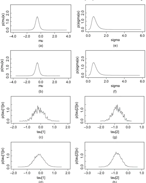
Fig. 2 compares posterior density estimates from the two two-stage analyses, purposely using
Table 1. Comparison of two-stage analyses with 1000 and 10 000 stage 1 samples to a one-stage analysis (pre-eclampsia data)†
Parameter Two-stage analysis Two-stage analysis One-stage (1000 samples) (10000 samples) analysis μ −0.51 (−1.11, 0.09) −0.51 (−1.12, 0.10) −0.51 (−1.11, 0.10) σ 0.68 (0.28, 1.56) 0.68 (0.27, 1.57) 0.67 (0.27, 1.57) τnew −0.51 (−2.26, 1.24) −0.51 (−2.28, 1.26) −0.51 (−2.25, 1.23)
†Posterior medians for overall parameters with 95% credible intervals in parentheses.
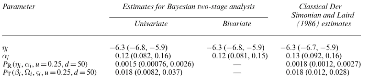
Table 2. Overall estimates (population medians) for main parameters of interest from Bayesian two-stage analysis of AAA data†
Parameter Estimates for Bayesian two-stage analysis Classical Der Simonian and Laird Univariate Bivariate (1986) estimates ηi −6.3 (−6.8,−5.9) −6.3 (−6.8,−5.9) −6.3 (−6.7,−5.9) αi 0.12 (0.082, 0.16) 0.12 (0.081, 0.15) 0.13 (0.092, 0.16) PR.ηi,αi,u=0:25,d=50/ 0.0015 (0.00076, 0.0026) — 0.0018 (0.0012, 0.0027)
PT.βi,Ωi,ςi,u=0:25,d=50/ 0.018 (0.0082, 0.037) — 0.018 (0.012, 0.028)
Study 1 2 3 4 5 6 7 8 9 Overall Two−Stage (1000 samples) sigma posterior median = 0.68 Two−Stage (10,000 samples) sigma posterior median = 0.68 One−stage
sigma posterior median = 0.67 Method Stage 1 Stage 2 (1000 samples) Stage 2 (10,000 samples) One−stage Stage 1 Stage 2 (1000 samples) Stage 2 (10,000 samples) One−stage Stage 1 Stage 2 (1000 samples) Stage 2 (10,000 samples) One−stage Stage 1 Stage 2 (1000 samples) Stage 2 (10,000 samples) One−stage Stage 1 Stage 2 (1000 samples) Stage 2 (10,000 samples) One−stage Stage 1 Stage 2 (1000 samples) Stage 2 (10,000 samples) One−stage Stage 1 Stage 2 (1000 samples) Stage 2 (10,000 samples) One−stage Stage 1 Stage 2 (1000 samples) Stage 2 (10,000 samples) One−stage Stage 1 Stage 2 (1000 samples) Stage 2 (10,000 samples) One−stage
Log odds ratio (95% CI) 0.04 (−0.75, 0.85) −0.15 (−0.82, 0.60) −0.13 (−0.81, 0.61) −0.13 (−0.80, 0.62) −0.92 (−1.60, −0.22) −0.82 (−1.47, −0.24) −0.82 (−1.46, −0.21) −0.82 (−1.45, −0.22) −1.14 (−1.97, −0.33) −0.92 (−1.71, −0.27) −0.93 (−1.71, −0.25) −0.94 (−1.72, −0.24) −1.53 (−2.68, −0.48) −1.12 (−2.11, −0.31) −1.10 (−2.10, −0.25) −1.08 (−2.08, −0.28) −1.41 (−2.14, −0.77) −1.19 (−1.86, −0.61) −1.20 (−1.87, −0.63) −1.20 (−1.86, −0.60) −0.30 (−0.54, −0.06) −0.30 (−0.54, −0.09) −0.31 (−0.54, −0.07) −0.31 (−0.54, −0.07) −0.27 (−0.96, 0.41) −0.34 (−0.98, 0.28) −0.33 (−0.96, 0.29) −0.33 (−0.95, 0.30) 1.20 (−0.37, 3.19) 0.19 (−0.79, 1.56) 0.18 (−0.79, 1.57) 0.16 (−0.82, 1.56) 0.14 (−0.38, 0.65) 0.03 (−0.44, 0.53) 0.04 (−0.46, 0.55) 0.03 (−0.46, 0.54) −0.51 (−1.11,0.09) −0.51 (−1.12,0.10) −0.51 (−1.11, 0.10) –2 –1 0 1 2 3
Log odds ratio
Fig. 1. Results of the two-stage and one-stage analyses of the pre-eclampsia data: estimates are posterior medians with 95% credible intervals; the medians are shown as squares with area inversely proportional to the posterior variance; the edges of the diamonds used to denote overall estimates correspond to the limits of the 95% credible interval, whereas the central vertices show the posterior median
the same bandwidth in both cases to emphasize the effect of the stage 1 posterior sample size.
Inferences on the overall parametersμandσare virtually identical, suggesting that these are
not strongly dependent on the number of stage 1 samples collected. Fig. 2 also shows density
estimates forτ1andτ2as examples of study-specific parameters. In the cases where only 1000
stage 1 samples have been used the density estimates are somewhat ‘granular’ because there are fewer values to choose from, which reduces the resolution with which the target density can be represented.
4.2. Abdominal aortic aneurysm data
BUGS code for the stage 1 analysis is given in the on-line appendix A.5. In practice, to
en-sure that the parameters are less correlated, all time variables (tijkandTij) are centred at the
mean follow-up time for the study, whereas, in the hazard function,ψ.bij,Tij/is centred at the
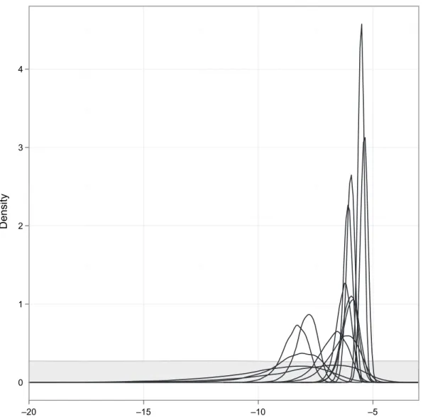
study mean AAA diameter. Transformations are then required to obtain common parameters across the studies. Such centring is not necessary but can improve convergence substantially. For monitoring convergence, each stage 1 analysis was conducted with two MCMC chains running in parallel; the method of Gelman and Rubin (Gelman and Rubin, 1992; Brooks and Gelman, 1998) was then used. A typical analysis involved a burn-in of 6000 iterations, with 100 000 further iterations thinned by 20. In all cases, sufficient iterations for obtaining 10 000 approximately independent posterior realizations for each study level parameter of interest were performed. Even with the aforementioned centring to improve convergence, each stage 1 anal-ysis took several hours to perform. Hence a single one-stage analanal-ysis of the full hierarchi-cal model would have taken of the order of days to perform. Bearing in mind that there are numerous parameters of interest in this setting, a two-stage approach was considered essen-tial. Prior distributions for all parameters, including derived parameters, were effectively flat within the range of values supported by the corresponding posterior, as illustrated in Fig. 3 for the log-odds of rupture within 3 months (0.25 years) given a baseline diameter of 50 mm,
logit{PR.ηi,αi,u=0:25,d=50/}.
At stage 2, to ensure comparability between studies, intercept parameters βi1 were
stan-dardized to represent a mean AAA diameter at t=0, whereas log-baseline-hazards ηi were
standardized to represent the log-hazard at a diameter of 40 mm. Both univariate and
bivar-iate two-stage analyses for the parametersηi andαi were performed. In addition, a range of
univariate two-stage analyses for the derived parametersPR.ηi,αi,u,d/andPT.βi,Ωi,ςi,u,d/
was conducted, specifically to make predictions for time periods of between 3 months and 2
years, in 3-month intervals (u=0:25, 0:5, 0:75, . . . , 2), for individuals with a diameter of 50 mm
(d=50). In each stage 2 analysis, 200 000 realizations were generated after an initial burn-in of
10 000 iterations (convergence was assessed by visual inspection of chain history plots and by Gelman and Rubin’s method in confirmatory analyses).
Table 2 shows the overall estimates for the basic parametersηi andαi. For comparison, a
classical random-effects summary estimate (DerSimonian and Laird, 1986) is also calculated by using the posterior medians and standard deviations from stage 1. Point and interval estim-ates for the overall parameters are similar between the Bayesian two-stage and the classical random-effects approaches. In addition, univariate and bivariate stage 2 analyses give almost identical results. The population mean log-baseline hazard (for an AAA diameter of 40 mm),
η, is low and signifies a median rupture rate, exp.η/, of 1.8 (95% credible interval 1.1–2.7) per
1000 person-years. However, the hazard increases significantly with diameter, with a population
median hazard ratio, exp.α/, of 1.13 (95% credible interval 1.09–1.17) per millimetre increase
in AAA diameter.
(a) mu –4.0 –2.0 0.0 2.0 4.0 p(mu| x ) 0.0 1.0 2.0 (e) sigma 0.0 2.0 4.0 6.0 p(sigma| x ) 0.0 1.0 2.0 (b) mu –4.0 –2.0 0.0 2.0 4.0 p(mu| x ) 0.0 1.0 2.0 (f) sigma 0.0 2.0 4.0 6.0 p(sigma| x ) 0.0 1.0 2.0 (c) tau[1] –2.0 –1.0 0.0 1.0 2.0 p(tau[1]| x ) 0.0 1.0 (g) tau[2] –3.0 –2.0 –1.0 0.0 1.0 p(tau[2]| x ) 0.0 1.0 (d) tau[1] –2.0 –1.0 0.0 1.0 2.0 p(tau[1]| x ) 0.0 1.0 (h) tau[2] –3.0 –2.0 –1.0 0.0 1.0 p(tau[2]| x ) 0.0 1.0
Fig. 2. Posterior density estimates forμ,σ,τ1andτ2based on 100000 stage 2 samples from analysis of the pre-eclampsia data: (a)p.μjxC,xT/by using 1000 stage 1 samples; (b)p.μjxC,xT/by using 10000 stage 1 samples; (c)p.τ1jxC,xT/by using 1000 stage 1 samples; (d)p.τ1jxC,xT/by using 10000 stage 1 samples; (e)p.σjxC,xT/by using 1000 stage 1 samples; (f)p.σjxC,xT/by using 10000 stage 1 samples; (g) p.τ2jxC,xT/by using 1000 stage 1 samples; (h)p.τ2jxC,xT/by using 10000 stage 1 samples
Health Service AAA screening programme, are invited back for re-screening after 3 months. To assess the appropriateness of this monitoring interval, we begin by calculating, for an individual with diameter 50 mm, the study-specific predicted probabilities of rupture and of crossing the
surgical intervention threshold (55 mm) within a 3-month period,PR.ηi,αi,u=0:25,d=50/
andPT.βi,Ωi,ςi,u=0:25,d=50/respectively. In the second stage, a hierarchical structure is
placed on the logit of each predicted probability, by assuming that the study-specific values originate from a common (normal) population distribution. Table 2 shows the overall estim-ates transformed back to the probability scale. These now have considerably wider credible
Log−odds of rupture within 3 months given 50mm diameter Density 0 1 2 3 4 –5 –10 –15 –20
Fig. 3. Kernel density estimates for all 14 stage 1 posteriors for the log-odds of rupture within 3 months (0.25 years) given a baseline diameter of 50 mm, logit{PR.ηi,αi,uD0:25,dD50/}, from independent analyses of study-specific AAA data: , prior distribution, scaled (arbitarily) so that it is visible on the same plot
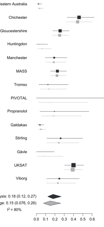
intervals than those obtained via classical random-effects meta-analysis. Results indicate that the current 3-month screening policy is relatively safe, with point estimates (and 95% credible intervals in parentheses) for the overall/population-median values of the probabilities of rup-ture before next screen and of crossing the intervention threshold within 3 months being 0.15% (0.076–0.26%) and 1.8% (0.82–3.7%) respectively. There is considerable between-study heter-ogeneity in these quantities, however, which raises the question of whether there are patient or study level characteristics that may explain this; however, this topic is not pursued here. To illustrate the level of heterogeneity, Fig. 4 shows a forest plot of the stage 1 and stage 2 pos-terior distributions (medians and 95% credible intervals) for the probability of rupture within 3 months, given a diameter of 50 mm. Note that study-specific estimates are variable, and that
those from stage 2, corresponding to the full hierarchical model, are generally more precise than those from stage 1. Considerable shrinkage is also apparent for several studies.
Fig. 5 shows the probabilities of rupture and of crossing the intervention threshold, given
d=50, for various values of the monitoring intervalu. These are obtained straightforwardly
by adapting the procedure that was outlined above foru=0:25. We can see that monitoring
intervals of 9 months or less and 6 months or less respectively are required to be confident that the population median probabilities of rupture and of crossing the intervention threshold are below 1% and 10%. However, given the degree of between-study variation, it would seem inappropriate to use this as a basis for justifying a longer monitoring interval.
5. Discussion
We have developed a novel method for analysing fully Bayesian hierarchical models in two stages; to the best of our knowledge this approach has not been used before. The method can be
thought of as a type of particle filter (sequential Monte Carlo sampling; Doucetet al.(2001);
Andrieuet al. (2010)), where the resampling is done via Metropolis–Hastings sampling; the
considerable literature on particle filtering may thus point to ways of improving or extending our method. Our approach is computationally efficient and can be easily applied in settings where a one-stage analysis is difficult or impossible (e.g. for complex parameters of interest) or inefficient (e.g. when there are multiple parameter sets of interest). Although we have demon-strated, here, that the method works for a simple binomial example, we have also tested it within various settings, such as Poisson regression, and have discovered no further issues. In addition, we can see no theoretical or intuitive reason why it should fail, as long as stage 1 posteriors are obtainable. Where applicable, our approach allows potentially complex problems to be broken down into a series of more manageable problems, facilitating, for example, individually tailored analyses for each study in stage 1, and allowing a wide range of inferences to be readily obtained following a single stage 1 analysis.
In cases where the parameters of interest are complex functions, such as the probability that is associated with some clinically relevant event, a two-stage approach offers a surprisingly sim-ple solution, avoiding the need for reparameterization of the model and subsequent reanalysis of all data. If an overall estimate of the parameter of interest is sufficient, and we require no heterogeneity measure, then another option might have been to estimate a posterior distribu-tion for the parameter of interest by transforming simulated values for the populadistribu-tion mean
parametersμfrom some basic analysis. However, the resulting quantity would not, in general,
be meaningful, since it would not normally represent the population mean or median value, say, or any other established measure of centrality, on the scale of interest (because, for example,
f.E[x]/=/ E[f.x/] for non-linearf.·/). Also, predictions on the scale of interest, for new studies,
say, would not be possible by using such an approach.
One limitation of our method is the requirement for the stage 1 posteriors, obtained under an assumption of marginal independence between studies, to provide reasonable approximations to the full conditional distributions for the study-specific parameters in the hierarchical model,
where studies are typically assumedconditionallyindependent instead, given the overall
param-eters. If there is too much conflict between these distributions then the Metropolis sampler may become degenerate, accepting only a few of the stage 1 samples. However, we would expect that this is unlikely to happen, since the most likely cause of such conflict is when shrinkage effects would be strong in the hierarchical model, owing to limited data from particular studies, in which case the corresponding stage 1 posteriors will be wider. In extreme cases, we may lose some resolution unless very large MCMC samples are taken of the posteriors from stage 1.
0.0 0.1 0.2 0.3 0.4 0.5 0.6 Probability of rupture (x 100) Western Australia Chichester Gloucestershire Huntingdon Manchester MASS Tromso PIVOTAL Propranolol Galdakao Stirling Gävle UKSAT Viborg
Classical D&L meta−analysis: 0.18 (0.12, 0.27) Bayesian two−stage: 0.15 (0.076, 0.26)
I2 = 80%
Fig. 4. Results of stage 1 ( , ) and stage 2 ( , ) analyses of AAA data for the probability of rupture within 3 months, given 50 mm diameter: the estimates are posterior medians with 95% credible intervals; the medians are shown as squares with an area inversely proportional to the posterior variance on the logit scale;I2is the proportion of total variation due to heterogeneity between studies; the diamond notation is for overall estimates as in Fig. 1
Time inter
val u (months)
Pr(rupture within inter
val u | diam = 50mm) 0.010 0.005 0.000 0.015 0.020 Time inter va l u (months)
Pr(cross threshold within interval u | diam = 50mm) 0.1 0.0
0.2 0.3 0.4 0.5 0.6 0 5 10 15 20 0 5 10 15 20 ( a ) ( b ) Fig. 5. P opulation median probabilities of clinically significant e v ents occurr ing within time per iods of betw een 3 and 24 months, in 3-month interv als: (a) probability of rupture giv en a diameter of 50 mm; (b) probability of crossing the surgical interv ention threshold giv en a diameter of 50 mm; estimates are posterior medians with 95% credib le interv als
Another limitation occurs when data are sparse and some of the stage 1 posteriors are thus improper. Hence they cannot be obtained for use as proposal distributions. The method pro-posed may, at least, be used partially for such data sets, with the units for which a stage 1 posterior is available handled as described in Section 3.2, and the remaining units modelled as they would be in a standard, one-stage analysis. (In such cases it is convenient to rearrange the data so that the units for which only sparse data are available form a contiguous block.)
Our method has been presented in a meta-analysis context but is an entirely general advance, which is applicable, in principle, to a wide range of hierarchical modelling scenarios. We have
implemented it in freely available software, OpenBUGS (www.openbugs.info), which is
sufficiently flexible that the user may apply the methodology to almost arbitrary problem types. As mentioned above, we require that the stage 1 posteriors are obtainable. One situation in which this is not so is when the ‘borrowing of strength’ that a hierarchical model permits is essential for the identification of unit-specific (study-specific in the case of meta-analysis) parameters. This can occur in population pharmacokinetics, for example, where longitudinal drug concen-tration data are available for a number of individuals and we wish to make overall inferences about the concentration–time relationship. Often, in the latter stages of drug development, many patients are followed but each may give rise to only one or two concentration measurements, thus precluding independent analyses of patient-specific data.
Model criticism within the framework proposed is an area for further exploration. Stan-dard approaches, such as traditional residual-based methods, and more advanced techniques
(e.g. Rizopoulos et al.(2010)) are applicable to stage 1 results, since stage 1 comprises
stan-dard analyses only. Within stage 2, study level residuals and predictive distributions are readily
obtained, facilitating the use of established methods for criticism, such as Bayesian p-values
(Gelman, 2003; Gelmanet al., 2004). Outlying studies could be accommodated or identified
by assuming a (multivariate) Studenttpopulation distribution for the parameters of interest
(e.g. Wakefieldet al.(1994)). The degrees of freedom could be either prespecified or estimated
as part of the analysis, the latter offering a means of assessing the appropriateness of a simpler normality assumption for the population distribution instead. Efficient ways of performing cross-validation (e.g. Marshall and Spiegelhalter (2003)) and computing the deviance
informa-tion criterion (Spiegelhalteret al., 2002) within stage 2 are currently under investigation.
Finally, it may be possible to extend the methodology to allow two-stage Bayesian modelling in more complex evidence syntheses, such as multiparameter evidence synthesis (Ades and
Sut-ton, 2006; Presaniset al., 2011; Sweetinget al., 2008), or mixed treatment comparisons (Salanti
et al., 2008; Lu and Ades, 2006).
Acknowledgements
This work was funded by the UK Medical Research Council and the National Institute for Health Research (grants MRC:U105260557 (to DL), MRC:G0902100 and MRC:U105261167 (to JB), National Institute for Health Research–Health Technology Assessment grant 08/30/02 (to MS) and MRC:U105200001 (to ST)). We thank Ian White, whose input was invaluable. We also thank the Joint Editor, Associate Editor and two referees, whose comments helped us to improve on an earlier version of the paper. We are also grateful to the RESCAN Collaboration
for permission to use their data in this methodological paper:researchers, Dr Matthew Bown,
Dr Louise C. Brown, Professor Martin J. Buxton, Professor F. Gerald Fowkes, Mr Matthew Glover, Dr Susan Gotensparre, Professor Roger Greenhalgh, Mr Tim Hartshorne, Dr Lois Kim, Professor Ross Naylor, Professor Janet T. Powell, Dr Michael J. Sweeting, Professor Simon G.
Western Australia, Mr S. Parvin, Royal Bournemouth Hospital, UK, Hilary Ashton, St Rich-ard’s Hospital, Chichester, UK, Mr R. Chalmers, Edinburgh Royal Infirmary, UK, Mr J. J. Earnshaw, Gloucestershire Royal Infirmary, UK, Mr A. B. M. Wilmink, University of Bir-mingham, UK, Professor J. A. Scott, University of Leeds, UK; Professor C. N. McCollum, University Hospital of South Manchester, UK, Dr S. Solberg, Rikshospitalet, Oslo, Norway, Dr K. Ouriel, New York-Presbyterian-Hospital, New York, and Medtronic Vascular, Santa Rosa, California, USA, Professor A. Laupacis, St Michael’s Hospital, Toronto, Canada, Dr M. Vega de Ceniga, Hospital de Galdakao, Spain, Mr R. Holdsworth, Stirling, UK, Dr L. Karlsson, Gavle, Sweden, and Dr J. S. Lindholt, Viborg, Denmark.
References
Ades, A. E. and Sutton, A. J. (2006) Multiparameter evidence synthesis in epidemiology and medical decision-making: current approaches (with discussion).J. R. Statist. Soc.A,169, 5–35.
Andrieu, C., Doucet, A. and Holenstein, R. (2010) Particle Markov chain Monte Carlo methods (with discussion). J. R. Statist. Soc.B,72, 269–342.
Brooks, S. P. and Gelman, A. (1998) General methods for monitoring convergence of iterative simulations.J. Computnl Graph. Statist.,7, 434–455.
Collins, R., Yusuf, S. and Peto, R. (1985) Overview of randomised trials of diuretics in pregnancy.Br. Med. J., 290, 17–23.
Cowles, M. K. and Carlin, B. P. (1996) Markov chain Monte Carlo convergence diagnostics: a comparative review. J. Am. Statist. Ass.,91, 883–904.
DerSimonian, R. and Laird, N. (1986) Meta-analysis in clinical trials.Contr. Clin. Trials,7, 177–188.
Doucet, A., de Freitas, N. and Gordon, N. (2001)Sequential Monte Carlo Methods in Practice. New York: Springer.
Gelfand, A. E. and Smith, A. F. M. (1990) Sampling-based approaches to calculating marginal densities.J. Am. Statist. Ass.,85, 398–409.
Gelman, A. (2003) A Bayesian formulation of exploratory data analysis and goodness-of-fit testing.Int. Statist. Rev.,71, 369–382.
Gelman, A., Carlin, J. B., Stern, H. S. and Rubin, D. B. (2004)Bayesian Data Analysis, 2nd edn. London: Chapman and Hall–CRC.
Gelman, A. and Rubin, D. B. (1992) Inference from iterative simulation using multiple sequences (with discussion). Statist. Sci.,7, 457–511.
Gilks, W. R. and Wild, P. (1992) Adaptive rejection sampling for Gibbs sampling.Appl. Statist., 41, 337– 348.
Hastings, W. K. (1970) Monte Carlo sampling-based methods using Markov chains and their applications. Bio-metrika,57, 97–109.
Higgins, J. P. T., Thompson, S. G. and Spiegelhalter, D. J. (2009) A re-evaluation of random-effects meta-analysis. J. R. Statist. Soc.A,172, 137–159.
Higgins, J. P. T., Whitehead, A., Turner, R. M., Omar, R. Z. and Thompson, S. G. (2001) Meta-analysis of continuous outcome data from individual patients.Statist. Med.,20, 2219–2241.
Ihaka, R. and Gentleman, R. (1996) R: a language for data analysis and graphics.J. Computnl Graph. Statist.,5, 299–314.
Lee, K. J. and Thompson, S. G. (2008) Flexible parametric models for random-effects distributions.Statist. Med., 27, 418–434.
Lu, G. and Ades, A. E. (2006) Assessing evidence inconsistency in mixed treatment comparisons.J. Am. Statist. Ass.,101, 447–459.
Lunn, D. J., Best, N., Thomas, A., Wakefield, J. and Spiegelhalter, D. (2002) Bayesian analysis of population PK/PD models: general concepts and software.J. Pharmkinet. Pharmdyn.,29, 271–307.
Lunn, D., Jackson, C., Best, N., Thomas, A. and Spiegelhalter, D. (2012)The BUGS Book: a Practical Introduction to Bayesian Analysis. Boca Raton: CRC Press.
Lunn, D., Spiegelhalter, D., Thomas, A. and Best, N. (2009) The BUGS project: evolution, critique and future directions (with discussion).Statist. Med.,28, 3049–3082.
Lunn D. J., Thomas, A., Best, N. and Spiegelhalter, D. (2000) WinBUGS—a Bayesian modelling framework: concepts, structure, and extensibility.Statist. Comput.,10, 325–337.
Marshall, E. C. and Spiegelhalter, D. J. (2003) Approximate cross-validatory predictive checks in disease mapping models.Statist. Med.,22, 1649–1660.
Mengersen, K. L., Robert, C. P. and Guihenneuc-Jouyaux, C. (1999) MCMC convergence diagnostics: a reviewww. InBayesian Statistics 6(eds J. M.Bernardo, J. O. Berger, A. P. Dawid and A. F. M. Smith), pp. 415–440. Oxford: Oxford University Press.
Metropolis, N., Rosenbluth, A. W., Rosenbluth, M. N., Teller, A. H. and Teller, E. (1953) Equations of state calculations by fast computing machines.J. Chem. Phys.,21, 1087–1091.
Neal, R. M. (1997) Markov chain Monte Carlo methods based on ‘slicing’ the density function.Technical Report 9722. Department of Statistics, University of Toronto, Toronto.
Presanis, A. M., De Angelis, D., Goubar, A., Gill, O. N. and Ades, A. E. (2011) Bayesian evidence synthesis for a transmission dynamic model for HIV among men who have sex with men.Biostatistics,12, 666–681. RESCAN Collaborators (2012) Meta-analysis of individual patient data to examine factors affecting growth and
rupture of small abdominal aortic aneurysms.Br. J. Surg.,99, 655–665.
Riley, R. D., Lambert, P. C. and Abo-Zaid, G. (2010) Meta-analysis of individual participant data: rationale, conduct, and reporting.Br. Med. J.,340, article c221.
Ripley, B. D. (1987)Stochastic Simulation. New York: Wiley.
Rizopoulos, D., Verbeke, G. and Molenberghs, G. (2010) Multiple-imputation-based residuals and diagnostic plots for joint models of longitudinal and survival outcomes.Biometrics,66, 20–29.
Salanti, G., Higgins, J. P. T., Ades, A. E. and Ioannidis, J. P. A. (2008) Evaluation of networks of randomized trials.Statist. Meth. Med. Res.,17, 279–301.
Smith, T. C., Spiegelhalter, D. J. and Thomas, A. (1995) Bayesian approaches to random-effects meta-analysis: a comparative study.Statist. Med.,14, 2685–2699.
Spiegelhalter, D. J., Best, N. G., Carlin, B. P. and van der Linde, A. (2002) Bayesian measures of model complexity and fit (with discussion).J. R. Statist. Soc.B,64, 583–639.
Sweeting, M. J., De Angelis, D., Hickman, M. and Ades, A. E. (2008) Estimating hepatitis C prevalence in England and Wales by synthesizing evidence from multiple data sources: assessing data conflict and model fit. Biostatistics,9, 715–734.
Sweeting, M. J. and Thompson, S. G. (2011) Joint modelling of longitudinal and time-to-event data with appli-cation to abdominal aortic aneurysm growth and rupture.Biometr. J.,53, 750–763.
Thompson, S., Kaptoge, S., White, I., Wood, A., Perry, P., Danesh, J. and the Emerging Risk Factors Collab-oration (2010) Statistical methods for the time-to-event analysis of individual participant data from multiple epidemiological studies.Int. J. Epidem.,39, 1345–1359.
Thompson, S. G. and Pocock, S. J. (1991) Can meta-analyses be trusted?Lancet,338, 1127–1130.
Wakefield, J. C., Smith, A. F. M., Racine-Poon, A. and Gelfand, A. E. (1994) Bayesian analysis of linear and non-linear population models by using the Gibbs sampler.Appl. Statist.,43, 201–221.
Supporting information
Additional ‘supporting information’ may be found in the on-line version of this article:
‘Supporting information for “Fully Bayesian hierarchical modelling in two stages, with application to meta-analysis”’.