Fabiano L. Ribeiro1,2, Joao Meirelles3,
Vinicius M. Netto4, Camilo Rodrigues Neto5, and Andrea Baronchelli2
Given that a group of cities follows a scaling law connecting urban population with socio-economic or infrastructural metrics (transversal scaling), should we expect that each city would follow the same behavior over time (longitudinal scaling)? This assumption has important policy implications, although rigorous empirical tests have been so far hindered by the lack of suitable data. Here, we advance the debate by looking into the temporal evolution of the scaling laws for 5507 municipalities in Brazil. We focus on the relationship between population size and two urban variables, GDP and water network length, analyzing the time evolution of the system of cities as well as their individual trajectory. We find that longitudinal (individual) scaling exponents are city-specific, but they are distributed around an average value that approaches to the transversal scaling exponent when the data are decomposed to eliminate external factors, and when we only consider cities with a sufficiently large growth rate. Such results give support to the idea that the longitudinal dynamics is a micro-scaling version of the transversal dynamics of the entire urban system. Finally, we propose a mathematical framework that connects the microscopic level to global behavior, and, in all analyzed cases, we find good agreement between theoretical prediction and empirical evidence.
1 Department of Physics (DFI), Federal University of Lavras (UFLA), Lavras MG, Brazil;
2 Department of Mathematics, City, University of London, UK;
3 Department of Civil and Environmental Engineering, Swiss Federal Institute of Technology Lausanne, Lau-sanne, VD, Switzerland;
4Universidade Federal Fluminense (UFF), Niter´oi, RJ, Brasil;
5School of Arts, Sciences and Humanities, University of Sao Paulo, Sao Paulo, SP, Brazil.
I. INTRODUCTION
An unprecedented abundance of data has significantly advanced our understanding of urban phenomena over the past few years [1–4]. These advances were also en-abled by the work of many theorists from different areas, such as physicists, urbanists and complex systems scien-tists, among others, who brought new insights and theo-ries to the field, resulting in a significant step towards a new science of cities [5].
A crucial finding concerns the scaling properties of ban systems. Empirical evidence has shown that an ur-ban variable, Y, scales with the population size N of a city, obeying a power law of the kindY ∝Nβ, whereβ is the scaling exponent quantifying how the urban met-ric reacts to the population increase [6–12]. On the one hand, the data revealed that socioeconomic urban vari-ables such as the number of patents, wages, and GDP present asuperlinear behavior in relation to the popula-tion size (β >1). Using the language of economics, one might say that this kind of urban variables exhibits
in-creasing returns to the urban scale. On the other hand,
infrastructure variables such as the number of gas sta-tions and length of roads scalesublinearly with the pop-ulation size (β <1). Finally, there is a third class of
vari-ables related to individual basic services, such as house-hold electrical and water consumption, and total employ-ment, which scales linearly with population size (β≈1). Among the various attempts to explain such behavior in urban phenomena [13–15], one of the most successful was proposed by Bettencourt and colleagues [16]. This theory proposes that urban scaling is a result of an inter-play between urban density and diversity, which are re-lated to economic competition and knowledge exchange, respectively. This is a consequence of the interaction be-tween the individuals that compose a city, resulting in innovation, economic growth, and economies of scale.
As these scaling laws have been observed in different countries [6–8, 10, 17–22] and periods of time [23, 24], some works also claimed that such patterns are, in fact, the manifestation of a universal law that would generally govern cities regardless of their context, culture, geog-raphy, level of technology, policies or history [9, 16, 20– 22, 25]. The universality proposition has been challenged [26–28], but most evidence seem to confirm the generality, while exceptions are normally explained by local partic-ularities [10, 18, 29, 30]. According to this proposition, in the long term, the general performance of a particular city would be greatly independent of individual - politi-cal - choices: the total amount of social interactions be-tween its citizens would guide, to a great extent, the city towards the observed scaling behavior. This proposition is unprecedented in urban science and the identification and validation of such universal dynamics could help ur-ban policymakers to identify opportunities and improve the life quality of dwellers.
A key open question is the difference in the scaling properties ofsingle cities andsystems of cities. Does an individual city growing in time follow the same scaling pattern observed for a snapshot of a group of cities? In the last years, few works have accurately focused on the dynamics of individual cities [31–34], while a growing lit-erature has been concentrating on the scaling properties of a set (system) of cities. We call the former
nalscaling properties, which take into account the evolu-tion of individual cities in time, and the latter transver-sal scaling across an urban system, i.e., computed from the set of cities that compose the system. Some recent works addressed this issue, reaching no unanimous con-clusion. For example, Depersin and Barthelemy analyzed the scaling exponent in time delays in traffic congestion in 101 US cities and found longitudinal scaling to be path-dependent on the individual evolution of cities and unrelated to the transversal scaling, challenging the uni-versality proposition [32]. In turn, Hong et al. argued that longitudinal and transversal exponents are corre-lated, but it is essential to eliminate global effects and properly measure the longitudinal scaling exponent [33]. Another work has found that the power-law scaling of 32 major cities in China could adequately be characterized for both transversal and longitudinal scaling [34]. More recent work also analyzed such an issue for the wage in-come in Sweeden and found superlinear scaling for both longitudinal and transversal scaling, but the former was characterized by larger scaling exponents [31].
Here, we will present our analysis of the transversal and longitudinal behavior of GDP and water network length (socio-economic and infrastructure variables, re-spectively) for 5507 Brazilian municipalities. Our main results show that the longitudinal scaling exponents are different from each other, as suggested by Depersin and Barthelemy’s work [32], but they are distributed around an average that approaches the transversal scaling expo-nent when the data are decomposed to eliminate external factors and when we consider only subsets of cities with a sufficiently large growth rate. Such results give support to the idea that the longitudinal dynamics is a micro-scaling version of the transversal dynamics of the entire urban system.
The paper is organized as follows: having posed the research problem in this section, we shall unfold our method and data used to assess the evolution of two dif-ferent urban metrics in section (II), namely GDP and water network length as a function of population size in different periods of time (from 1998 to 2014) for 5507 municipalities in Brazil. Section (III) brings details of the theoretical approach used to describe the dynamics of such properties as an analogous problem of particles in a vector field, applied in a way to render the relation between longitudinal and transversal scaling exponents clearer. In this section, we also explore the implications of our findings, along with potential contributions. Fi-nally, we draw our conclusions in section (IV).
II. EMPIRICAL EVIDENCE
Data of the Brazilian Urban System and its Scaling properties
The data presented here refer to 5507 Brazilian mu-nicipalities, with contiguous dense surrounding areas
ag-gregated in single spatial units from the totality of 5570 Brazilian administrative divisions. Data were collected from the website of theBrazilian Institute of Geography
and Statistics (IBGE)[35] and from the
water-sewage-waste companies national survey (SNIS)[36]. The present work will be restricted to two urban metrics, one for each scaling regime: i)GDP, a socio-economic variable that presents a superlinear behavior typically with the pop-ulation size and ii)water supply network length, an in-frastructure variable which has a sublinear behavior typ-ically.
A recent work [10] has shown that over 60 variables for the Brazilian urban system are well described by a power-law equation of the form:
Yi(t) =Y0(t)Ni(t)βT. (1)
Here, the time-dependent variables Yi(t) and Ni(t) are relative to the cityi; the former represents some urban metric (for instance GDP or water network length) and the latter represents the city population size. The two pa-rameters in Eq. (1) are the intercept parameterY0(t) and the transversal scaling exponentβT, which are obtained by the fit of this power law with the urban system data. These two parameters have to do with themacro-scale
properties of the urban system and, at first, do not repre-sent the particularities of a single city - themicro-scale. As we will show in the next sections, the intercept param-eter is a time-dependent variable, while the transversal scaling exponent can or cannot be time-dependent.
Transversal Scaling
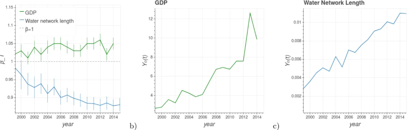
Fig. (1) shows the GDP as a function of the population size for different years (from 1998 to 2014) of our Brazil-ian municipality subset. The straight lines in Fig. (1) are the best fit (by the maximum likelihood method) of the Eq. (1) for different years. The transversal scaling exponentβT (the slope) of each line in Fig. (1) is always greater than one, indicating a persistent superlinear be-havior. Moreover, the best fit lines are visually paral-lel, that is,βT is approximately constant, even with the time evolution of studied municipalities, which reveals the robustness of the scaling exponent. These facts can be observed in more detail in Fig. (2-a), which presents the time evolution of βT for the Brazilian municipality subset. The transversal scaling exponent stays approxi-mately constant even with the intercept parameterY0(t) continuously increasing with time (see Fig. (2-b)).
Fig. (2) also presents the time evolution of the transversal scaling exponentβT for the water supply net-work length (in blue). In this case,βT is not constant and decreases over time, as seen in Fig. (2-a) while remain-ing smaller than 1, which was expected given it refers to an infrastructure variable. According to the available data, it is hard to establish whether its value will stabi-lize or not. The fact that this variable is not constant
FIG. 1: Scaling relation between population and GDP for Brazilian municipalities, from 1998 (blue) to 2014 (yellow). The straight lines are the best power-law equation fits for each year (by the maximum likelihood method). The straight lines are virtually parallel, which shows that the transversal scaling exponent is constant and robust. The scaling exponent is always greater than 1 for all years, with a mean ¯βT = 1.04. It reveals a superlinear scaling property, compatible with the fact that the GDP is a socio-economic urban variable. The numeric time evolution of the transversal scaling exponent and the intercept parameter are shown in Fig. 2.
could suggest that the urban system is still out of bal-ance with respect to this urban metric, as suggested by Pumain’s theory [14]. Moreover, the data suggest that the intercept parameter Y0(t) of this urban metric, as it was observed in GDP, maintains a continuous growth through the observed time frame (see Fig. (2-c)).
Longitudinal Scaling
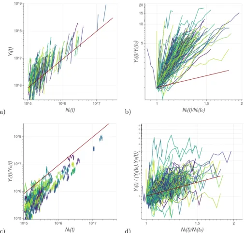
We now focus on the individual evolution of Brazilian municipalities. Fig. (3) presents different ways of ob-serving the longitudinal dynamics of the GDP and the population size for the municipalities subset. Fig. (3-a) presents the raw longitudinal trajectories, while Fig. (3-b) presents them re-scaled as Yi(t)/Yi(t0), as a function ofNi(t)/Ni(t0), following the idea proposed in [32]. The re-scaled form allows us to compare in one single image the slopes of the municipalities’ trajectories. Here, t0 is the first year that the data are available. One can see that municipalities experience different slopes, and in all cases, the exponent is greater than the transversal one (given by βT and represented by the dark red line in
Fig. (3-b)). Similar evidence was reported recently by Depersin and Barthelemy [32], which analyzed the tem-poral dynamics of delay in traffic congestion in US cities. They observed as we did here, that the individual dy-namics do not collapse in a single and universal curve, suggesting that longitudinal scaling in cities is not gov-erned by a single universal scaling exponent as the global system is.
Individual municipalities are being pushed by the growth of the global intercept parameterYi(t) and will rise in the lnY−x−lnN plane, having higher slopes than the global one. One way to deal with this is to decom-pose the longitudinal trajectory, graphing not lnYi(t) in the ordinate, but instead. lnYi(t)−lnY0(t), that is ln(Yi(t)/Y0(t)), in order to eliminate global effects, as suggested by [33]. The decomposed longitudinal trajec-tory is shown in Fig. (3-c), and its re-scaled form is pre-sented in Fig. (3-d). The slopes observed on the decom-posed and re-scaled form of the longitudinal trajectories are compatible with the transversal slope, represented by the dark red line in Fig. (3-d).
Lets callβithe scaling exponent of thei-th city, that is, the slope of the (raw) trajectories described in Fig. (3a-b) calculated using the longitudinal evolution ofYi(t) with
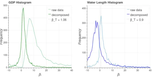
Ni(t). Similarly, we can compute the individual decom-posed scaling exponent, sayβidec, computed using the de-composed longitudinal trajectory described in Fig. (3c-d). Fig. (4) presents the distribution of the individual slope, for both sets{βi}i and{βidec}i, for GDP and wa-ter supply network length, for all studied municipalities. One can see that the decomposed individual slopes for GDP are distributed around the global slope, suggesting that the decomposed version of individual trajectories recover the transversal phenomena for GDP in Brazilian municipalities. Moreover, it suggests that regardless of each municipality having different dynamics, that is, dif-ferent longitudinal scaling exponentsβidec, their distribu-tion presents a mean value compatible with the transver-sal scaling exponent.
However, in the case of the water supply network length, the average of the distribution of the non-decomposed data is closer to the transversal slope than the decomposed one, suggesting that decomposition don’t recover the transversal scaling exponent for every urban variable. It is possible that this is the case because the transversal scaling exponent βT for water network length is not stable across the studied years. These re-sults suggest that the decomposition alone is not enough to infer that the individual and the global systems follow the same scaling properties in every case. In the next sections, we will introduce a theoretical approach that suggests that, in order to have an agreement between transversal and longitudinal scaling, it is also necessary to consider a new ingredient: the city growth rate.
a) b) c)
FIG. 2: a) Time evolution of the transversal scaling exponent βT for the GDP (green) and water supply network length (blue) for Brazilian municipalities. In the GDP case, there is no significant change of this parameter over the years and the regime (superlinear) is always sustained. In the case of water supply network length, βT is always smaller than 1, which is expected, given the infrastructure nature of this metric, and it is decreasing over time. b) and c) present the time evolution of the intercept parameterY0(t) for GDP and water supply network length, respectively. The intercept parameter is constantly growing for both urban metrics.
III. THEORETICAL APPROACH
In this section, we present a theoretical approach to de-scribe urban metrics dynamics. In order to do so, we will treat the dynamics of the urban metrics as an analogous problem of particles in a vector field. Fig. (5) presents the plane lnY-x-lnN and the two-dimensional “move-ment” of one single city – a “particle” – as a result of the
vectors acting in the horizontal or vertical direction.
In the horizontal direction there is a vector represent-ing an increase in the city’s population size. It is coloured in green in Fig. (5) and has a magnitude ∆ lnNi(t), where we have introduced the compacted notation:
∆ lnNi(t)≡lnNi(t+ ∆t)−lnNi(t), (2) as it was suggested in [33]. In the vertical direction of this plane we have vectors acting on the increment of the urban metric (GDP or water supply network length, for instance). We will consider, by hypothesis, that there are at least two distinct vectors acting in this direction. The first, let’s say Fint, represented by the red vector in Fig. (5), is an extensive quantity Whose magnitude is a direct response to the increase in population size. This vector has to do with theagglomeration effect that came from the interaction between the individuals who belong to this single city. The second, let’s say Fext, represented by the blue vector in Fig. (5), is the result of all external mechanisms such as, for instance, some wealth/knowledge that comes from other cities or re-gions; it can also represent the result of the interaction between individuals who belong to this single city with dwellers from other cities; or even some individual incor-porated ability that increases the individual productivity. Therefore, the resulting vector acting on the vertical direction of the plane, sayFtot, is the sum of these two
vectors, that is:
Ftot=Fint+Fext, (3)
which has a magnitude
Ftot= ∆ lnYi(t)≡lnYi(t+ ∆t)−lnYi(t). (4) The action of this vector field (in the horizontal and vertical directions) during a time interval ∆t conducts to a “displacement” ∆r(t) of this city (or particle) in the two-dimensional plane lnY-x-lnN. But let us try to identify these vectors with the empirical variables avail-able.
The data presented in the previous section suggest that we have an empirical law that governs the cities, which can be described by the expression (1). If this equation is a law, then any theory that is formulated to describe scaling properties in cities must be constrained to follow it. As this equation holds for any timet, we can write it for the next time instantt+ ∆t, that is:
Yi(t+ ∆t) =Y0(t+ ∆t)Ni(t+ ∆t)βT(t+∆t). (5) Then, by extracting the logarithm of the ratio Yi(t+ ∆t)/Yi(t) and using Eqs. (1) and (5) we are conducted to: ∆ logYi(t) = log Y0(t+ ∆t) Y0(t) + ( ¯βT +)∆ logNi(t). (6) where we used the compacted forms defined on (2) and (4). Moreover, we also introduced ¯βT as the av-erage value of the transversal exponent during the time interval ∆t, and the parameter, which is a quantity pro-portional to the differenceβT(t+∆t)−βT(t). In fact, the data analysis suggests thatis sufficiently small for the cases we are studying here, so it will be neglected in our
a) b)
c) d)
FIG. 3: Different forms to see the longitudinal dynamics of the GDP and the population size for all Brazilian municipality subsets. Each trajectory represents the time evolution of one single urban area, from the year 1998 to 2014. a) log-log plot of the time evolution of the raw data of GDP as a function of the population size. The dark red straight line is the power-law equation, with the average transversal scaling exponent ¯βT = 1.05. b) log-log plot of the re-scaled form of the longitudinal dynamics, which allows us to compare the slopes of the cities’ trajectory. This graph shows us that cities have different slopes, and they are greater than ¯βT, represented by the dark red line. c) Decomposed longitudinal trajectory, which allows seeing the dynamics without global effects. d) Decomposed and re-scaled form of the longitudinal dynamics, which shows that the individual slopes are compatible with the transversal scaling exponent, represented by the dark red line. The distribution of the individual slopes (for raw and decomposed data) can be seen in Fig. (4).
analyses. WhenβT(t) is constant, as it is approximately the case for GDP dynamics, then= 0.
The elements of Eq. (6) can be identified with the vec-tors presented in Fig. (5) and consequently with Eq. (3). It allows us to identify: Fext= log Y0(t+ ∆t) Y0(t) (7) and Fint= ( ¯βT+)∆ logN(t). (8) The external vector, since it is directly computed from the ratio between the final and initial intercept param-eter, can be interpreted as a measurement of the global growth of the urban metric. In this sense, the value given by (7) is an average value of the external vector. That is: typically, a city in the system has an external vector
magnitude given by the value computed from (7). In the last section, when we decomposed each city’s evolution into a relative change, we removed external factors act-ing on each city and consideract-ing only internal factors (the ones that come from agglomeration effects). In relation to the magnitude of the internal vector, it is an extensive variable; that is, it is a direct response to the increase of the population size. These results suggest that, in order for the urban metric to depend only on the population size (under the formY = cte·NβT), it is necessary for βT to be constant ( → 0) and Fext →0, which means absence of global growth. That can be the case for some urban metrics, but of course, it is not the case for GDP and many other variables. Our theoretical approach sug-gest thatβdec
i 6=βT when6= 0, which was observed in our empirical data for the water supply network length.
FIG. 4: Histogram of the longitudinal scaling exponent sets {βi}i (raw data) and{βidec}i (decomposed data) for GDP and water network length for all Brazilian municipality subsets. For GDP (on the left), the decomposed data are distributed around the transversal scaling exponentβT (vertical dashed line), suggesting that it makes sense to decompose this urban variable. However, in the case of water network length (on the right), the distribution of the raw (non-decomposed) data is closer to the global slope than the distribution of the decomposed one, suggesting that decomposition is not working for this urban variable.
FIG. 5: Plane lnY-x-lnN, which represents the “movement” of the city as a particle in a vector field. In the horizontal direction, we have the vector (green) that represents the in-crease in population size. In the vertical direction there is the action of two vectors: Fint (red), which is an extensive quantity whose magnitude is a direct response to the incre-ment of the population size related to an agglomeration effect between the individuals that live in this single city; andFext (blue), which is the vector related to some external aspects, or the interaction between the individuals from this city with individuals of other cities, or some individual incorporated ability. The action of this vector field during a time interval ∆tconducts to a “displacement” ∆r(t) of this city (or parti-cle) in this two-dimensional plane. The two parallel lines are given by the global system (transversal) power law (Eq. (1)) intandt+ ∆t.
Relation between transversal and longitudinal scaling exponents
With the approach presented above, it is possible to write a relation between the transversal and the longi-tudinal scaling exponent. Given that the longilongi-tudinal scaling exponentβi is obtained by:
βi=
∆ lnYi(t) ∆ lnNi(t)
, (9)
then if we divide Eq. (6) by ∆ lnNi(t), we have:
βi=βT ++
Fext lnbi
, (10)
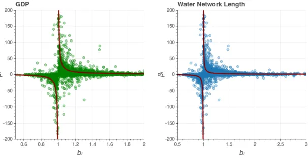
wherebi≡Ni(t+∆t)/Ni(t) is the city population growth rate. The graphs in Fig. (6) show that this result works very well when we analyzeβias a function ofbi, for both GDP and water supply network length for the studied municipalities. It shows a strong dependence between these two variables.
The result (10) also suggests that if Fext > 0 and
bi > 1, which means that both the intercept parame-ter (global growth) and the population are growing with time, thenβiwill always be greater than the global expo-nentβT. The increment in the intercept implies a more accentuated slope of the city trajectory in the plane lnY -x-lnN (that is, bigger βi) in relation to the transversal trajectory (related toβT), in accordance with the empir-ical observation presented in this study as well as other evidences presented in recent literature [32–34]. More-over, longitudinal and transversal scaling will be the same when only internal factors (agglomeration effects) are acting on the system (Fext= 0).
In urban scaling analysis, it is important to know the value of the scaling exponent because it gives us the effi-ciency and productivity of the city or the urban system (given byβiandβT, respectively) since it shows how the urban metric reacts to an increase in population. For instance, in socio-economic variables, larger values ofβ
mean a more productive city, and for infrastructure vari-able, smaller values means a more efficient city. How-ever, in the context we are analyzing, cities with very large values of βi are not necessarily more productive. In fact, large values of scaling exponents are related to cities with a very low growth rate (according to Eq. (9)), so the value of βi is not useful for the main purpose of seeing how productivity or scaling economies emerge.
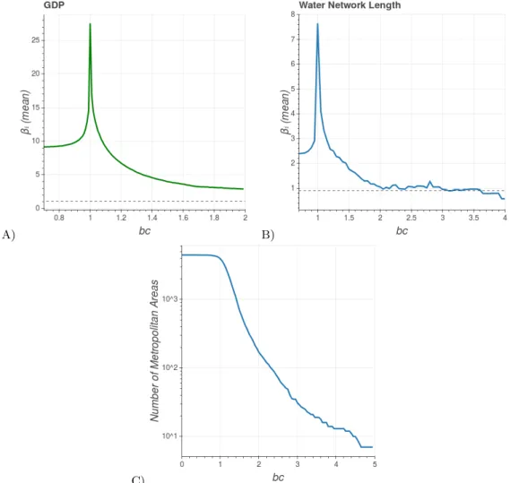
However, we believe that the value of βi will informs about the city’s efficiency when it has a sufficiently large population growth rate. In order to investigate this, we computed the average values of the longitudinal scal-ing exponents ¯βi, using only cities with bi greater than a threshold bc, and later built the graph presented in Fig. (7), where we can see that ¯βi decreases drastically for greater values ofbc, approaching the transversal expo-nent value for both GDP and water network length. This result suggests that when we consider a city that has grown significantly during the time period analyzed, it is relevant to understand its longitudinal scaling growth properties as a microscopic version of the macroscopic growth of the urban system. Another important aspect of these findings is that onlydecompositionis not enough to link globally with longitudinal scaling, as highlighted in the last section. In fact, decomposition only makes sense if we consider cities with sufficient growth in a given period of time, or with constant transversal scaling ex-ponentβT (6= 0).
The results presented here must be confronted with more urban metrics and other countries. Moreover, a problem resulting from the approach presented in this section concerns the small number of municipalities that present bc sufficiently large. For instance, in order to compute the average ¯βi forbc >4 we used only 13 mu-nicipality subsets (see Fig. (7-c)). The statistics could be improved if we were studying an urban system with more municipalities experiencing higher growth rates, but maybe such systems don’t even exist. Thus a more feasible situation for future analyses consists of finding a way to normalize the longitudinal scaling exponent to the city’s growth rate.
The external Vector
Eq. (7) represents the average magnitude of the exter-nal vector, that is, a city within the system will have an external vector with magnitude typically given by this value. However, it is interesting to know about the spe-cific external vector value acting on an individual city. This is a very difficult matter to be resolved given that it involves particularities of the city, but we can infer its
answer by the data that we have available.
For instance, we can use the result given by Eq. (10) to infer the external vectorFi
extrelative to the i-th city. That is, we can write that:
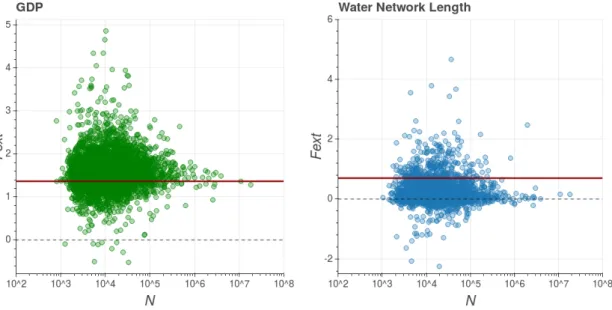
Fexti = (βi−βT −) lnbi, (11) and ifβT, βi (given by Eq. (9)) andbi are known, then it is possible to estimate (assuming≈0) the individual external vector. That is the case presented by Fig. (8), where each dot represents the value obtained for the ex-ternal vector of a single municipality, for both GDP and water network.
Fig. (8) also presents the comparison between this in-dividual and the average external vector magnitudes. It suggests an interesting aspect differentiating these two urban metrics’ dynamics. In the case of GDP, the cities of all sizes are distributed around the average magnitude of the external vector. However, in the case of water sup-ply network length, bigger cities present external vector smaller than the average. These characteristics imply dif-ferent dynamics with respect to the transversal exponent, according to the schematic drawing in Fig. (9), which presents the plane lnY-x-lnN with two scenarios for the external vectors. In the first scenario, the external vec-tor is approximately the same for all cities of the system, regardless of their size; it implies that the slope of the fit line (in lnY-x-lnN plane) remains constant. That is more or less what happens in the GDP context of the Brazilian municipalities. It suggests an equilibrium situ-ation, or at least that this urban variable is in a mature state inside the system.
In the second scenario, the external vector is smaller for bigger cities, which implies that the slope of the fit line decreases over time. That is apparently the case for the water network of the Brazilian municipalities. One possible explanation is that the system is still out of equi-librium. That is, water network length in Brazil is not mature yet, and maybe it will converge to the equilibrium (when the magnitude of the external vector of all cities will be around an average value) given enough time. In any case, in order to have a better understanding of that aspect, further research about these observations is nec-essary, which can be achieved by following the evolution of more urban variables.
IV. CONCLUSION
We analyzed the longitudinal and transversal scaling dynamics of 5507 Brazilian municipalities, aggregated with contiguous dense surrounding municipalities from the totality of municipalities. We showed, using two ur-ban metrics - GDP and water supply network length - That the longitudinal scaling exponents are different from each other, but they are distributed around an av-erage that approaches the transversal scaling exponent when we remove external factors (by decomposition) and when we consider cities that grew sufficiently during the
FIG. 6: Graph ofβias a function of the population growth ratebi, for both GDP (on the left) and water network length (on the right). Each dot represents the data of a single Brazilian municipality subset and the red curve is the theoretical prediction given by Eq. (10) using: = 0 for both cases;βT = 1.15 for GDP; andβT= 0.9 for water network length. This result illustrates the strong dependence between the longitudinal scaling exponent and the population growth rate of the city. It also suggests that cities with biggerβi are the ones with little or no growth (bi ≈1). Moreover, bi <1 (decreasing population) implies a negativeβi.
analyzed period. We then proposed a formal vectorial de-scription that describes under which conditions longitu-dinal (βi) and transversal (βT) scaling should converge or where we can expect discrepancies. This result supports the hypothesis that longitudinal and transversal urban dynamics could be differently scaled versions of the same phenomenon. However, in order to have a more conclu-sive argumentation, further investigation is required with other urban variables and other countries.
Acknowledgments
We would like to acknowledge all colleagues from the Mathematical Department of City, University of Lon-don, where most of the work was done. FLR acknowl-edges the members of CASA-UCL, especially the
stimu-lating discussions with Elsa Arcaute during his sabbat-ical year in 2017. Also, thanks to the Brazilian agen-cies CAPES (process number: 88881.119533/2016-01) and CNPq (process number: 405921/2016-0) for finan-cial support.
Author Contributions
FLR, JM, and AB conceived the project; FLR, JM, and AB designed research; FLR and JM curated the data; FLR and JM analyzed the data; FLR, JM, VMN, CRN, and AB analyzed and interpreted the results; FLR and JM elaborated the formal analysis; FLR wrote the orig-inal draft; FLR, JM, VMN, CRN, and AB read, and commented on, the manuscript.
[1] M. Batty, “Building a science of cities,” Cities, vol. 29, 2012.
[2] G. B. West, Scale: the universal laws of growth, inno-vation, sustainability, and the pace of life in organisms, cities, economies, and companies. Penguin, 2017. [3] L. M. A. Bettencourt, “the Uses of Big Data,”SFI
Work-ing Paper, pp. 12–22, 2013.
[4] M. Barthelemy, The structure and dynamics of cities. Cambridge University Press, 2016.
[5] M. Batty,The new science of cities. MIT Press,, 2013. [6] L. G. A. Alves, H. V. Ribeiro, E. K. Lenzi, and R. S.
Mendes, “Distance to the Scaling Law: A Useful Ap-proach for Unveiling Relationships between Crime and Urban Metrics,”PLoS ONE, vol. 8, no. 8, 2013. [7] L. M. Bettencourt and J. Lobo, “Urban scaling in
eu-rope,” Journal of The Royal Society Interface, vol. 13, no. 116, p. 20160005, 2016.
[8] L. M. A. Bettencourt, J. Lobo, D. Helbing, C. K¨uhnert, and G. B. West, “Growth, innovation, scaling, and the pace of life in cities.,” Proceedings of the National Academy of Sciences of the United States of America, vol. 104, pp. 7301–6, apr 2007.
A) B)
C)
FIG. 7: Graph A) and B): mean value of the longitudinal scaling exponent (for GDP and water network length) as a function of the growth rate thresholdbc. The parameterbc delimits the cities that will be used to compute the average. The mean value of ¯βidecreases drastically as bc increases. Moreover the greaterbc is the more ¯βiapproaches toβT (represented by the dashed line). It’s reasonable to think that in an ideal situation with no external forces and with a significant number of cities with the larger growth rate for better statistics, the average of the longitudinal scaling exponent will converge to the value of the transversal scaling exponent. Graph C: number of metropolitan areas used to compute the mean as a function ofbc. This number is drastically smaller for greaterbc values.
[9] E. Strano and V. Sood, “Rich and poor cities in Europe. An urban scaling approach to mapping the European eco-nomic transition,” PLoS ONE, vol. 11, no. 8, pp. 1–8, 2016.
[10] J. Meirelles, C. R. Neto, F. F. Ferreira, F. L. Ribeiro, and C. R. Binder, “Evolution of urban scaling: Evidence from brazil,”PloS one, vol. 13, no. 10, p. e0204574, 2018. [11] A. Gomez-Lievano, H. Youn, and L. M. Bettencourt, “The statistics of urban scaling and their connection to zipf’s law,”PloS one, vol. 7, no. 7, p. e40393, 2012. [12] C. K¨uhnert, D. Helbing, and G. B. West, “Scaling laws
in urban supply networks,” Physica A: Statistical Me-chanics and its Applications, vol. 363, pp. 96–103, apr 2006.
[13] A. Gomez-Lievano, O. Patterson-Lomba, and R. Haus-mann, “Explaining the prevalence, scaling and variance of urban phenomena,”Nature Human Behaviour, vol. 1, no. 1, p. 0012, 2017.
[14] L. J. Pumain D, Paulus F, Vacchiani-Marcuzzo C, “An evolutionary theory for interpreting urban scaling laws,” Cybergeo: European Journal of Geography;, 2006. [15] F. L. Ribeiro, “An attempt to unify some population
growth models from first principles,” Revista Brasileira de Ensino de Fisica, vol. 39, no. 1, pp. 1–11, 2017. [16] L. M. A. Bettencourt, “The origins of scaling in cities.,”
Science, vol. 340, no. 6139, pp. 1438–41, 2013.
[17] A. F. Van Raan, G. Van Der Meulen, and W. Goedhart, “Urban scaling of cities in the netherlands,”PLoS One, vol. 11, no. 1, p. e0146775, 2016.
[18] A. Sahasranaman and L. M. Bettencourt, “Urban geog-raphy and scaling of contemporary indian cities,” Jour-nal of the Royal Society Interface, vol. 16, no. 152, p. 20180758, 2019.
[19] P. Adhikari and K. M. de Beurs, “Growth in urban extent and allometric analysis of west african cities,”Journal of land use science, vol. 12, no. 2-3, pp. 105–124, 2017.
FIG. 8: Magnitude of the external vector as a function of population size for every single Brazilian municipality in our subset. On the left, we have data referring to GDP and on the right to water network length. The dots represent Fi
ext computed from the expression (11) while the red line represents the average magnitude of this vector over the system, computed by the expression (7). The dashed line isFext= 0. In the case of GDP, the municipality subsets of all sizes are distributed around the average value, but in the case of the water network length, the greater subsets presented external vector smaller than the average. These particularities imply different dynamics of the transversal scaling exponent, as shown in Fig. (9).
FIG. 9: Schematic drawing representing the plane lnY-x-lnN with two scenarios for the external vectors. In the first scenario (on the right), the magnitude of the external vectors is the same regardless of city size; implying that the slope of the fit line (in lnY-x-lnN plane) remains constant from t to t+ ∆t. That is more or less what happens in the GDP of the Brazilian municipalities, revealing that this urban variable is in a mature state in the system. In the second scenario (on the left), the external vector is smaller for bigger cities, which implies that the slope of the fit line decreases with time (fromtto ∆t). That is apparently the case for the water network length of the Brazilian municipalities, suggesting that this urban metric is not mature in the system.
[20] R. Louf, C. Roth, and M. Barthelemy, “Scaling in trans-portation networks,” PLoS ONE, vol. 9, no. 7, pp. 1–8, 2014.
[21] A. Gomez-Lievano, H. J. Youn, and L. M. Bettencourt, “The statistics of urban scaling and their connection to Zipf’s law,”PLoS ONE, vol. 7, no. 7, 2012.
[22] A. Gomez-Lievano, O. Patterson-Lomba, and R. Haus-mann, “Explaining the Prevalence, Scaling and Variance of Urban Phenomena,”Nature Human Behaviour, vol. 1, no. 0012, pp. 1–6, 2016.
[23] S. G. Ortman, A. H. F. Cabaniss, J. O. Sturm, and L. M. A. Bettencourt, “The pre-history of urban
scal-ing,”PloS one, vol. 9, no. 2, p. e87902, 2014.
[24] R. Cesaretti, J. Lobo, L. M. Bettencourt, S. G. Ort-man, and M. E. Smith, “Population-area relationship for medieval european cities,” PloS one, vol. 11, no. 10, p. e0162678, 2016.
[25] F. L. Ribeiro, JoaoMeirelles, F. F. Ferreira, and C. R. Neto, “A model of urban scaling laws based on distance-dependent interactions,” Royal Society Open Science, vol. 4, no. 160926, 2017.
[26] E. Arcaute, E. Hatna, P. Ferguson, H. Youn, A. Johans-son, and M. Batty, “Constructing cities, deconstructing scaling laws,” Journal of The Royal Society Interface, vol. 12, no. 102, p. 20140745, 2015.
[27] C. Cottineau, E. Hatna, E. Arcaute, and M. Batty, “Di-verse cities or the systematic paradox of Urban Scal-ing Laws,”Computers, Environment and Urban Systems, vol. 63, pp. 80–94, 2017.
[28] C. C. Cottineau, E. Hatna, E. Arcaute, and M. Batty, “Paradoxical Interpretations of Urban Scaling Laws,” arXiv preprint arXiv:1507.07878, no. July, pp. 1–21, 2015.
[29] E. Strano and V. Sood, “Rich and poor cities in europe. an urban scaling approach to mapping the european
eco-nomic transition,”PloS one, vol. 11, no. 8, p. e0159465, 2016.
[30] N. Z. Muller and A. Jha, “Does environmental policy affect scaling laws between population and pollution? evidence from american metropolitan areas,” PloS one, vol. 12, no. 8, p. e0181407, 2017.
[31] M. Keuschnigg, “Scaling trajectories of cities,” Proceed-ings of the National Academy of Sciences, p. 201906258, 2019.
[32] J. Depersin and M. Barthelemy, “From global scaling to the dynamics of individual cities,” pp. 1–6, 2017. [33] I. Hong, M. R. Frank, I. Rahwan, W.-S. Jung, and
H. Youn, “A common trajectory recapitulated by urban economies,” 2018.
[34] S. Zhao, S. Liu, C. Xu, W. Yuan, Y. Sun, W. Yan, M. Zhao, G. M. Henebry, and J. Fang, “Contemporary evolution and scaling of 32 major cities in China,” Eco-logical Applications, vol. 28, no. 6, pp. 1655–1668, 2018. [35] Instituto Brasileiro de Geografia e Estat´ıstica,
https://www.ibge.gov.br/
[36] SNIS: National system of information on sanitation. Elec-tronic version: app.cidades. gov.br/serieHistorica/