NBER WORKING PAPER SERIES
FIRST IN THE CLASS? AGE AND THE EDUCATION PRODUCTION FUNCTION Elizabeth Cascio
Diane Whitmore Schanzenbach Working Paper 13663
http://www.nber.org/papers/w13663
NATIONAL BUREAU OF ECONOMIC RESEARCH 1050 Massachusetts Avenue
Cambridge, MA 02138 December 2007
We thank Bruce Sacerdote for helpful conversations. We are also grateful to Joshua Angrist, Sandra Black, Kristin Butcher, David Card, Damon Clark, Ethan Lewis, Jens Ludwig, Heather Royer, Douglas Staiger, and seminar participants at Case Western Reserve University, Dartmouth College, the Federal Reserve Bank of San Francisco, the University of Florida, Wellesley College, the Association for Public Policy Analysis and Management Fall Conference, and the Society of Labor Economists Annual Meeting for comments on an earlier draft. All errors are our own. The views expressed herein are those of the author(s) and do not necessarily reflect the views of the National Bureau of Economic Research. NBER working papers are circulated for discussion and comment purposes. They have not been peer-reviewed or been subject to the review by the NBER Board of Directors that accompanies official NBER publications.
© 2007 by Elizabeth Cascio and Diane Whitmore Schanzenbach. All rights reserved. Short sections of text, not to exceed two paragraphs, may be quoted without explicit permission provided that full credit, including © notice, is given to the source.
First in the Class? Age and the Education Production Function Elizabeth Cascio and Diane Whitmore Schanzenbach
NBER Working Paper No. 13663 December 2007, Revised July 2012 JEL No. I20,J18,J24
ABSTRACT
We estimate the effects of having more mature peers using data from an experiment where children of the same age were randomly assigned to different kindergarten classrooms. Exploiting this experimental variation in conjunction with variation in expected kindergarten entry age to account for negative selection of older school entrants, we find that exposure to more mature kindergarten classmates raises test scores up to eight years after kindergarten, and may reduce the incidence of grade retention and increase the probability of taking a college-entry exam. These findings are consistent with broader peer effects literature documenting positive spillovers from having higher-scoring peers and suggest that – contrary to much academic and popular discussion of school entry age – being old relative to one’s peers is not beneficial. Elizabeth Cascio Department of Economics Dartmouth College 6106 Rockefeller Hall Hanover, NH 03755 and NBER [email protected] Diane Whitmore Schanzenbach School of Education and Social Policy Northwestern University
Annenberg Hall, Room 205 2120 Campus Drive
Evanston, IL 60208 and NBER
I. Introduction
In 1968, only four percent of U.S. six year olds were not in first grade. By 2010 this figure had risen to almost 20 percent.1 Only one-third of the recent trend is estimated to be explained by increases in the minimum kindergarten entry ages established by U.S. states; the rest is thought to be due to teachers deeming more kindergartners unready to progress to first grade, and to more parents choosing to delay their child’s entrance into school (Deming and Dynarski, 2008). Estimates over the past fifteen years put the rate of delay as high as 9 to 10 percent (e.g., West, Meek, and Hurst, 2000).
Anecdotally, the parental decision to delay is motivated by concerns that a child will be permanently disadvantaged if not among the biggest and brightest of his peers when he starts kindergarten. Being old or mature relative to one’s classmates can matter for
achievement over the long term if children are tracked early on the basis of skill, which is strongly correlated with age when children are young. Placement in the top academic track can be self-reinforcing, since it may tackle more advanced material and move more quickly through a given curriculum. At the same time, older school entrants might become relatively more motivated for school or self-confident because of their relative standing in the class. Importantly, the implied result is zero-sum: when older students gain, younger students lose, becoming less engaged with school, being placed on lower academic tracks, etc. This can create an unsustainable “race to the top” (see Gootman, 2006, and Weil, 2007).
Is there any evidence to support such zero-sum consequences of delayed school entry? Older school entrants do perform better on tests than younger school entrants in the same grade, even as late as middle school.2 However, this performance differential alone is
1 These are the authors’ tabulations from the 1968 and 2010 October Current Population Survey (CPS) School
Enrollment Supplements. For the purposes of this calculation, we record the small number of individuals in second grade or higher as being in first grade.
2 Bedard and Dhuey (2006) show this for a number of countries using data on fourth and eighth graders from
the 1995 and 1999 Trends in International Mathematics and Science Study (TIMSS). Similar findings have been documented in country-specific studies of the United States (Datar, 2006; Elder and Lubotsky, 2009), Sweden
not conclusive evidence that relative age matters: Older kindergartners have greater
preparation for school in an absolute sense, not just in relation to their peers; age also signals cognitive development as well as the flow of investments made in a child over his lifetime, so that older entrants’ edge on tests, even in middle school, may not even have anything to do with school per se.3 Direct estimates of relative age effects call for information on the ages of a child’s peers, which is generally lacking in the survey data frequently used in this
literature. As a result, there is limited evidence to date on whether children are better positioned to succeed if they are old relative to their peers when they start school.
We address this identification problem using data from one of the largest educational experiments ever undertaken in the United States – Tennessee’s Project STAR (Student-Teacher Achievement Ratio). Though designed to study the effects of reduced class size (Schanzenbach, 2007), Project STAR is well suited for estimating the effects of relative age.4 In particular, the design of Project STAR allows us to observe children who entered school at the same age, but were randomly assigned to kindergarten classmates with different ages on average. We can also follow these children over time. While such an exercise would be feasible in other data, such as matched student-teacher administrative data, Project STAR helps to ensure that variation in relative age is random. In a non-experimental setting, by contrast, concerned parents may lobby to have their children placed in kindergarten
classrooms where they would be relatively old. Our empirical strategy also accounts for the possible negative selection of delayed school entrants by exploiting variation across students
(Fredriksson and Öckert, 2006), Chile (McEwan and Shapiro, 2008), and Germany (Puhani and Weber, 2005), among others.
3 In fact, the impossibility of separately estimating the effects of age at school entry and age at test or
observation on elementary school test scores is cited by Angrist and Pischke (2009, p. 7) as an example of a “fundamentally unidentified question.” Black et al. (2011) separate the effects of age at school entry and age at test or observation by estimating these for army entrance exams given to young adults.
4 We are not the first to exploit the random assignment of children and teachers in Project STAR to classes, not
just to class sizes, to gain insights into the education production function (Dee, 2004; Dee and Keys, 2004; Whitmore, 2005; Schanzenbach, 2006; Chetty et al., 2011). Others have also exploited the random assignment of students and teachers to classes of different sizes to estimate peer effects (Boozer and Cacciola, 2001; Graham, 2008).
in anticipated school entry age given exact date of birth and Tennessee’s birthday cutoff for kindergarten entry. Our estimates therefore isolate the effects of variation in maturity across students of different ages in kindergarten, separately from variation in their innate ability.
We find little evidence to support the hypothesis that there are benefits to being relatively mature at the start of school. Children who are more mature relative to their
kindergarten classmates appear to lose out along every observed dimension: they score worse on achievement tests, both at the end of kindergarten and in middle school, are more likely to have been retained in grade by middle school, and are less likely to take a college-entrance exam, though the latter effects are estimated less precisely. Thus, our findings suggest, on net, positive spillovers from having more mature classmates in kindergarten. Maturity could have positive spillover effects through several channels. As noted above and also shown below, more mature children score higher on tests, particularly at the start of school. In addition, more mature children should be more ready for a given curriculum and are
therefore potentially less disruptive.5 While our findings are surprising from the perspective of academic and popular discussion of school entry age effects, they are therefore broadly consistent with the peer effects literature.
II. Background
Our analysis will focus on test performance and several other academic outcomes of one school entry cohort. The model of interest is:
(1) yit 0t 1tai 2t f
ai,i
itwhere yit represents an outcome for individual i in year t, and ai is his observed age (in years) in the fall of kindergarten. In this application, as in most in this literature, ai is perfectly
5 A number of studies have found that exposure to higher-achieving or less disruptive peers has benefits for a
child’s own achievement and behavior. On the effects of exposure to higher-achieving peers, see Hanushek et al. (2003), Ding and Lehrer (2007), Duflo et al. (2011), and Kugler et al. (2012). Figlio (2007) and Carrell and Hoekstra (2010), provide evidence that exposure to more disruptive peers can be harmful. See Sacerdote (2011) for a complete review of this literature.
correlated with the age at which an outcome is measured, ait. We therefore refer to their combined effect, β1t, as the “absolute age effect.” f
, represents relative age, taking as arguments own age ai and the vector of ages of child i’s peers, А-i; we refer to its coefficient, β2t, as the “relative age effect.” Thus, relative age is some function of a child’s own age and the ages of his peers. itrepresents unobserved determinants of the outcome of interest.Most studies to date have lacked data on А-i, and hence have omitted relative age when estimating model 1. As a result, most existing estimates of the coefficient on ai are reduced-form, capturing the effects of both absolute age and relative age. This has generated considerable uncertainty about correct interpretation in the literature. The interpretation of this reduced-form coefficient nevertheless has important implications. If the coefficient on age is truly a relative age effect, the implications of delaying school entry are zero-sum: the decision to delay one student’s entry into school improves his standing in the class at the expense of lowering everyone else’s. On the other hand, if the reduced-form coefficient on age represents an absolute age effect, such negative spillovers from the decision to delay do not exist.
We tackle the question of interpretation by using a data set where we observe the ages of each respondent’s peers at the start of school.6 Thus, we are able to measure relative age and control for it when estimating model 1. Yet, two questions arise in specifying this model.
First, what is the correct way to measure a child’s relative age? For simplicity and consistency with closely related literature on the United States (Elder and Lubotsky, 2009), we assume that f
ai,i
ai ai, where ai represents the average age of a i’s peers.
6 An alternative approach would be to impose functional form restrictions to support one interpretation over
another. For example, in one of the earliest papers in this literature, Bedard and Dhuey (2006) argue that their positive estimates of the coefficient on age for eighth-grade test scores capture the effect of relative age – not age at school entry – on the basis of a model where the effect of age at school entry is assumed non-linear.
Thus, we assume that relative age is linear, continuous, increasing in own age, and decreasing in the average age of peers. This captures the zero-sum implications of manipulating relative age. For example, in order for a given student to become relatively old, another student must become relatively young. Alternatively, if a child who would have otherwise been the
youngest among his peers waits an additional year to start school, he becomes the oldest only by virtue of making his peers relatively younger. As defined, relative age thus has implications for the distribution of achievement, but not its level.
Second, which peers determine relative age effects? Because of data constraints described below, we focus on relative age in the kindergarten classroom. A drawback of this definition is that we are only able to detect whether within-classroom interactions in
kindergarten drive relative age effects, not whether relative age effects exist at all. For example, if age in relation to classmates determines placement into reading groups, but children do not learn to read until first grade or later, we may not detect relative age effects when they truly exist, or our estimates of relative age effects could be biased downward. We explore the sensitivity of our estimates to the choice of peer group by estimating models where relative age is defined in relation to a child’s first-grade classmates, and the results are little changed.7 We also consider models where relative age is defined in relation to other children in the entire entry cohort of a child’s elementary school, and not just his own class. The latter models capture the possibility that children who are relatively young in their cohorts are likely to be among the youngest in their classrooms at some point during their elementary-school careers, and potentially repeatedly. They also capture the possibility that school administrators, not just teachers, target the youngest students in a cohort for lower academic tracks. These estimates rely less on the experimental variation in class assignment
in our data – in the latter case, no experimental variation is used at all – but they do provide potential insights into causal mechanisms.
Our approach is similar to Elder and Lubotsky’s (2009) study using survey data from the U.S. in which they measure relative age at the school cohort level in kindergarten, not the classroom level.8,9 However, they also address a fundamentally different question by using a different source of identifying variation in relative age. Elder and Lubotsky rely primarily on variation across states in the minimum age at school entry to generate variation across individuals in the average age of peers, and hence relative age. By contrast, our identification is based off of transitory (and random) fluctuations in the age distributions of kindergarten classrooms within schools, hence holding minimum age at school entry regulations constant. We describe how the source of identifying variation might affect interpretation when we present estimates of peer effects at the school cohort level below.
III. Empirical Strategy
Our primary estimates focus on a child’s relative age in his kindergarten classroom and, for ease of estimation and to parallel the peer effects literature, are based on the following model:
(2) yitk 0t 1tai 2tai,k xikt itk.
yitk now represents the outcome of individual i in year t who was assigned to classroom k in kindergarten, and ai remains his observed age at the start of kindergarten. Given that Project STAR included only one academic cohort and all students were tested (or observed) at the same time, ai is perfectly correlated with the age at which outcomes are measured. We are therefore only able to identify their combined effect, as noted above. ai,k is the average age
8 Fredriksson and Öckert (2006) use administrative data from Sweden to estimate a version of model 1 where
relative age is measured as child’s rank in the age distribution of his ninth-grade school cohort.
9 In principle, there are other situations where relative age varies while absolute age remains constant. For
example, changes in the minimum age at school entry change the expected relative age of some children without changing the year in which they should enter school (see Bedard and Dhuey, 2012).
of a child’s kindergarten classmates; xik is a vector including fixed (predetermined) characteristics of the individual, other (predetermined) characteristics of his kindergarten classmates, characteristics of his teacher, and class size; and εitk denotes unobserved determinants of outcomes.
As shown in Elder and Lubotsky (2009), the effect of relative age, ai ai,k, can be obtained simply by re-expressing model 2:
(2′) yitk 0t 1tai 2t
ai ai,k
xikt itkwhere 0t 0t, 1t 1t 2t and 2t 2t. Thus, the relative age effect is 2t 2t, where 2tis the effect of peer average age on outcomes at time t from model 2. The
expectation is that 2t 0. In words, holding constant own (entry) age, being relatively old improves academic outcomes; alternatively, holding constant own (entry) age, having older peers lowers outcomes on average (2t 0). The absolute age effect, 1t 1t 2t, is the sum of the coefficients on own and peer average age in model 2. Thus, if the relative age effect is positive, we would expect the coefficient on ai to fall relative to its value in the more commonly estimated specification where relative age is omitted from the model.
A comparison of models 2 and 2′ makes clear that a relative age effect is
indistinguishable from the effect of having less mature peers. Having less mature peers may improve a child’s position in the classroom “pecking order” – the positive spillover that we conceive of as a “relative age effect.” But it may also have negative spillovers, e.g., by exposing a child to lower-performing or more disruptive peers. Thus, even though we can re-express the parameters in model 2 to derive a relative age effect – as in model 2′ – the
coefficient is inherently a reduced-form one, capturing the net effect of these competing spillovers. It is important to keep this reduced-form interpretation in mind as we proceed.
t 2
Two identification problems arise when estimating model 2, both of which we can address. First, because kindergarten retention and delay are at the discretion of parents and teachers, older kindergartners may differ in unobservable ways from younger kindergartners, leading ordinary least squares (OLS) estimates of 1t to be biased. In particular, children delayed or retained are likely negatively selected, imparting a downward bias on OLS
estimates. We take the same empirical approach as previous researchers to this identification problem, constructing an instrument for ai using information on a child’s birthday and the date by which new school entrants are to reach a specified age.10 In particular, children in the Project STAR cohort were to have turned age five on or before September 30. As a result, a child who turned five on September 30 should have enrolled in kindergarten a month before, while her counterpart who turned age five on October 1 is expected to have entered kindergarten about one month before her sixth birthday.
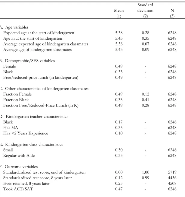
The solid line in Figure 1 illustrates the relationship between birthday and this “expected” age at the start of kindergarten, eai, under the assumption that the school year begins September 1. The figure shows clearly that actual age on September 1, 1985 (daily averages of which are represented by the hollow circles) is strongly but not perfectly related to eai. Two-stage least squares (TSLS) estimates of 1twill be consistent if eai is uncorrelated with unobserved determinants of achievement, or if E
eaiitk|xikt
0.11 While we cannot test this assumption directly, we show below that expected age at the start of kindergarten generally does not predict a child’s observed characteristics.
10 See, for example, Bedard and Dhuey (2006) and Elder and Lubotsky (2009), among others. A similar
approach can be used to construct an instrument for years of completed schooling in models of youth test scores (e.g., Gormley and Gayer, 2005; Cascio and Lewis, 2006) and of adult outcomes (e.g., Dobkin and Ferreira, 2010; McCrary and Royer, 2011).
11 A sufficient condition for this assumption to be satisfied is that birthday is randomly assigned, but it is
possible to identify 1t under weaker assumptions, e.g., under the assumption that expected school-entry age is
randomly assigned conditional on some flexible function of birthday that is smooth through the cutoff date. We have estimated a model like this as a robustness check and found similar results to those reported below (results available on request).
Second, there is likely to be sorting of children across kindergarten classrooms, possibly on unobservable characteristics related to the ages of other children. Our use of experimental data implies that no such sorting should have taken place, in which case
ai,k itk|xik t
0E . However, even with random assignment, older peers may be on average relatively low ability because some of these children will have been held back by their parents or teachers on the basis of their perceived school readiness. Thus, OLS estimates of 2tpick up the effects of having lower-ability peers in addition to the effects of having more mature peers.
To ensure that the peer effect we identify derives from maturity rather than ability, we combine the identification strategy described above with the random variation in classroom assignment from Project STAR. Specifically, we instrument for ai,k with the average expected age of a child’s peers, eai,k. Given the strong correlation between eai and ai shown in Figure 1, it is not surprising that we find a strong correlation between these
variables. This instrument should also be valid because variation in the birthday composition of a child’s classmates should be uncorrelated with his latent academic potential due to the experimental design. As above, we can informally test this assumption by examining the relationship between eai,k and observables.
Thus, while the OLS and TSLS estimates of 2tare in principle both unbiased, they are estimates of different parameters. The explanation is intuitive: given that older classmates may have been delayed or previously retained in kindergarten, OLS estimates of 2t pick up not just the effect of having more mature classmates in kindergarten, but also the effect of having “overage” classmates in kindergarten, who are likely of below average ability. By contrast, the TSLS estimates identify how having peers of the same innate ability but different
levels of maturity at the start of school affects the average child’s academic performance. The TSLS estimates therefore have a cleaner interpretation.
IV. Data
A. Sample and Summary Statistics
Project STAR was an experiment designed to study the effects of class size on student achievement. Kindergarten students and teachers in 79 Tennessee schools were randomly assigned to three different class types – small (with target enrollment of 13-17 students), regular (with target enrollment of 22-25 students), and regular with a full-time teacher’s aide – in the fall of 1985.12 This cohort was to have maintained its class type through third grade, after which all participants were returned to regular-sized classes. Random assignment of children to class types took place within schools.
Our analysis exploits the fact that most, if not all, Project STAR participants would have been randomly assigned to classrooms, not just class types, as a result of the
experimental design. We focus on peers in the kindergarten classroom because non-random transitions across class types (and classrooms) were less problematic in kindergarten than they would later become.13 However, we do estimate model 2 at the first grade classroom level in a robustness check. We also estimate model 2 at the school-cohort level for
comparison to Elder and Lubotsky (2009), but these estimates do not rely in any way on the experiment.
12 Children entering the experiment in grades one through three, either by moving into the school or having
been retained in grade the previous year, were also added to existing classes through random assignment. Each of the 79 schools had enrollment sufficient to accommodate at least one class of each type and were thus slightly larger than the state average. To ensure sufficiently large samples of poor and minority children, Project STAR schools were also disproportionately drawn from inner cities. A comparison of Project STAR schools to other Tennessee schools is provided in Schanzenbach (2007).
13 Using administrative data for 18 Project STAR schools, Krueger (1999) found that only five of 1581
participants did not attend their initially assigned class type in kindergarten. As the experiment continued, however, ten percent of students made transitions across class types. Anecdotally, these class switches were largely the result of student misbehavior, which might plausibly be related to age at school entry or the average age of kindergarten classmates.
We restrict our estimation sample to participants for whom each of the available background characteristics (birthday, race, gender, free lunch status in kindergarten) and kindergarten teacher characteristics (experience, education, and race) is observed.14 However, to construct average age and other characteristics of kindergarten classmates, we use all available data on the Project STAR kindergarten cohort, not just those individuals with non-missing outcomes data.
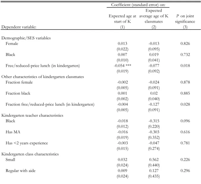
Table 1 gives summary statistics on these students and their teachers in our estimation sample. As has been found in nationally-representative data, children in our sample tend to be older at the start of kindergarten than expected (5.43 years old versus 5.38 years old), as shown in Panel A. However, the sample is not nationally representative. As shown in Panel B, nearly half of Project STAR participants received free or reduced-price lunch in kindergarten, and 33 percent were black (Panel B). By comparison, only 15.4 percent of five year olds in the U.S. were black in fall 1985.15 About 17 percent of
kindergarten teachers were black, 35 percent had master’s degrees, and 10 percent had less than 2 years of experience (Panel D). Students were roughly equally divided across class size types (Panel E).
Our main outcomes come from tests administered to STAR participants through the end of high school. In the spring of kindergarten, STAR participants were administered the Stanford Achievement Test.16 For participants still attending public school in Tennessee, we have scores on the Comprehensive Test of Basic Skills (CTBS) in grades 5 through 8,
14 This results in us dropping only 75 observations. The observations dropped are not significantly predicted,
individually or jointly, by the instrumental variables for age and average age of peers.
15 There are authors’ calculations from the 1985 October CPS School Enrollment Supplement.
16 Scores on the Stanford Achievement Test are also available for STAR participants in grades 1 through 3 who
did not leave a STAR school or repeat or skip a grade during the experiment. Unfortunately, our instrumental variables are related to attrition during the experiment, so we are unable to use these data. This is most likely driven by the relationship of these variables to grade repetition (shown below), but we are not able to observe the reason that children attrite from the sample, so we cannot confirm this.
regardless of year attended.17 Both tests are multiple-choice standardized tests with reading and math components. We average the reading and math scale scores on each test, then standardize this average to have a mean of zero and a standard deviation of one using data on all STAR participants with non-missing test scores in a given year. Thus, coefficient estimates in the test-score models are in standard deviation (σ) units. The last panel of Table 1 shows that the kindergartners in our sample are slightly positively selected from the pool of all Project STAR participants, scoring on average 0.12σ above the mean in spring 1994. This positive selection may arise because it was not mandatory for the Project STAR cohort to attend kindergarten, and kindergarten attendees may have been positively selected.
Our analysis focuses on test scores at the end of kindergarten (in spring 1986) and in spring 1994, when STAR participants progressing through school normally would have been completing eighth grade. We choose spring 1994 because many existing studies have
considered the relationship between age and test scores in eighth grade. We present estimates for the year that the cohort was expected to be in eighth grade instead of eighth-grade test scores because our sample includes individuals in the same school-entry cohort, and we wish to have our estimates be consistently interpretable across tests taken at different points in time. Because either one of the treatment variables may have affected grade
progression, we also estimate separate models for whether a child was enrolled below eighth grade when tested in spring 1994. One quarter of students tested are deemed to have been retained by this measure (Panel F).
Our final outcome measure is an indicator for whether a respondent took the ACT or SAT college-entrance exam. College-entry test information on STAR participants was collected from graduating classes through 1999 (i.e. for students who graduated early,
17 This is true as long as a child attended grades 5 through 8 at some point between 1990-91 and 1996-97. Test
scores were also collected in 1989-90, but are not available for a large, non-random subset of children who attended school in Memphis because the tests were not universally given there in that year.
time, or no later than one year behind “normal” grade progression) from all high schools in the U.S.18 Perhaps not surprisingly, individuals in our sample are less likely to have taken the ACT or SAT (47 percent) than individuals in the U.S. overall (lower panel of Table 1).19 B. Is Variation in the Instruments Exogenous?
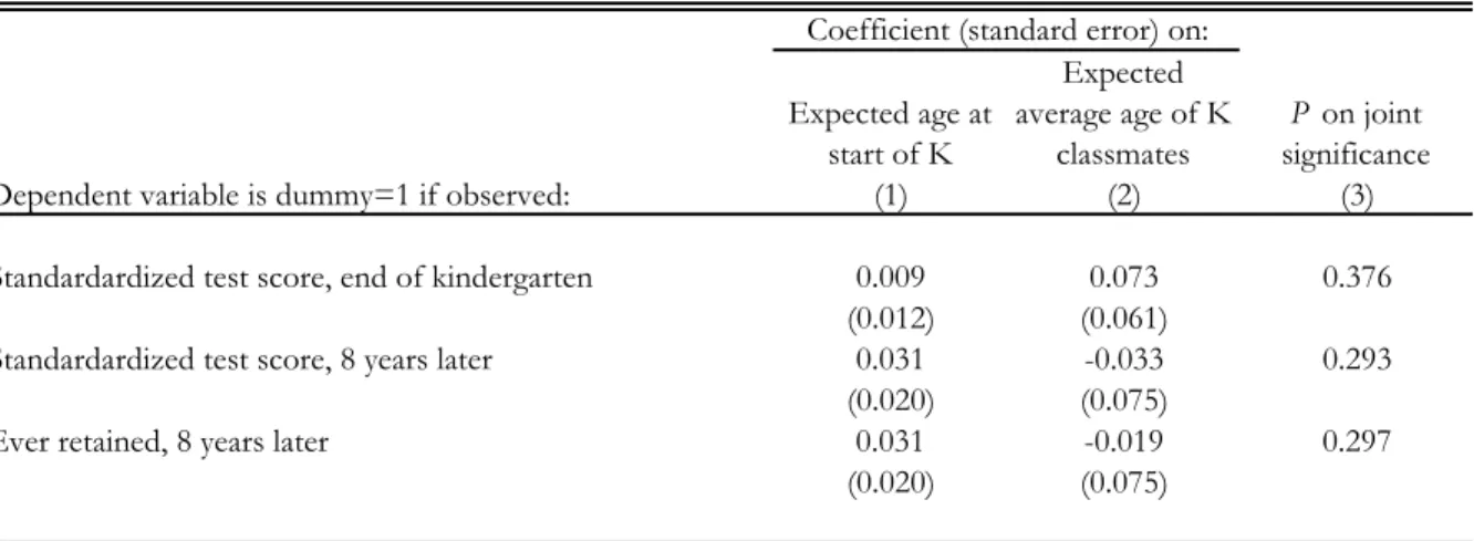
Before turning to the estimates, it is useful to demonstrate that expected age at school entry appears to be randomly assigned and to establish that the experiment generated random variation in the average expected age of a child’s kindergarten classmates. To this end, Table 2a gives the coefficients on eai and eai,k, along with their joint significance, in models where observed characteristics are the dependent variables. In Table 2b, we present the results from a similar exercise where the dependent variables are instead indicators for whether several key outcomes are observed.20 The underlying regressions also include school fixed effects, because random assignment of children to class types took place within
schools. Standard errors are consistent for heteroskedasticity and correlation of error terms among children in the same kindergarten classroom.
The estimates are consistent with random assignment. As shown in Table 2a, in only one case does expected age predict an observed correlate of test scores (column 1,
respondent receipt of free or reduced price lunch), and in no instance does the average expected age a respondent’s peers significantly predict his own background or the average background of his peers, or his kindergarten teacher or class characteristics (column 2).21 The instruments are jointly significant for only three of thirteen variables, and in one of these
18 See Krueger and Whitmore (2001) for more information about how the CTBS and college entrance exam
data were collected. Observation of other outcomes, like high school grades, is selected on our instrumental variables.
19 For example, using the National Longitudinal Educational Study, Bedard and Dhuey (2006) report an
ACT/SAT test-taking rate of 60 percent.
20 ACT or SAT test-taking is observed for all Project STAR participants.
21 The specification checks in Chetty et al. (2011), which include a wider range of background characteristics
that are not available to us in this study, also support random assignment to kindergarten classrooms in Project STAR. We have also re-estimated our models on students attending the only kindergarten class of its size within their schools (where assignment should have been random). The estimates are noisier, but broadly consistent with those reported below for the full sample (results available on request).
cases (teacher race), only marginally so (column 3). As shown below, including these variables as controls has little impact on the TSLS estimates. Table 2b shows that the instruments also do not predict observation of our dependent variables. This suggests that observations with missing values of dependent variables are random with respect to the identifying variation in ai and ai,k, and that the estimates presented below are not biased by sample selection.
V. Results
A. Conventional Estimates
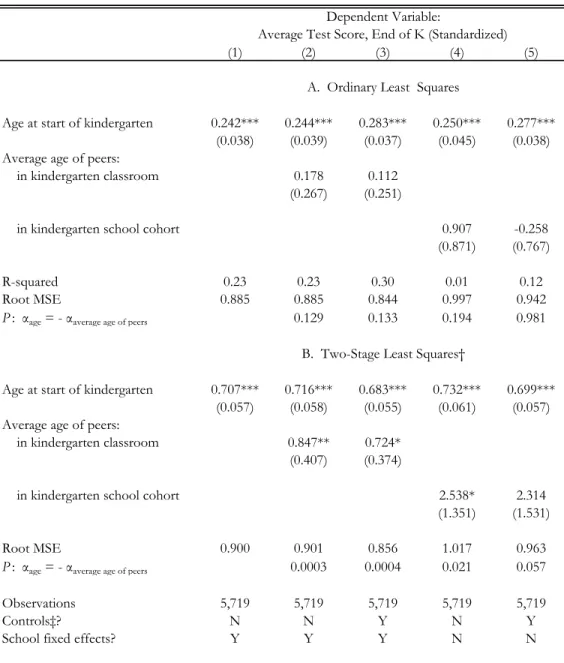
Table 3 presents OLS and TSLS estimates of the coefficients on own age and peer average age from model 2. The dependent variable is the standardized average of math and reading scores at the end of kindergarten. Unless otherwise noted, all specifications hereafter include fixed effects for school attended in kindergarten, and estimation accounts for
heteroskedasticity and arbitrary correlation of error terms within kindergarten classrooms. We first present estimates of the coefficient on age at kindergarten entry from a version of model 2 that excludes ai,k. This model is the same as that widely estimated in the school entry age literature, and so provides a useful benchmark. The OLS estimates, shown in Panel A, imply that STAR participants who were one year older at the start of kindergarten scored on average 0.24σ higher on a standardized test at the end of kindergarten (column 1). However, these estimates will be biased if children previously retained or delayed in entering kindergarten are selected on unobservables. As described above, we confront this possibility by comparing children who should have entered
kindergarten with a one-year difference in age, given their birthdays; if birthday is randomly assigned, these children will be on average identical in all other ways. As shown in Panel B of the same column, TSLS estimates using expected age at kindergarten entry as an instrument
imply that the test-score differential between two otherwise identical children who enter kindergarten with a one-year difference in age is a significantly higher 0.71σ.22
These estimates are comparable to those previously found in
nationally-representative data for the U.S. For example, applying a similar identification strategy to data on a more recent kindergarten cohort, Elder and Lubotsky (2009) find that an additional year of age at school entry is associated with a 0.87σ difference in math test performance and a 0.61σ difference in reading test performance in the spring of a child’s kindergarten year.23 Like us, Elder and Lubotsky (2009) and Bedard and Dhuey (2006) also find that OLS estimates of the coefficient on age are significantly lower than their TSLS counterparts, suggesting that students who are older by actual age (but not predicted age) are negatively selected. When we estimate similar models for test scores at the end of eighth grade, we also obtain findings that are quite similar to those previously documented for the U.S.24 Unlike Bedard and Dhuey (2006), however, we do not find that older school entrants are more likely to take a college entrance exam.25 In general, however, the consistency of our
estimates with the existing literature suggests the possible broader applicability of inferences made from our data.
22 First-stage estimates for the specifications in Table 3 are presented in Table A1.
23 When we estimate separate models by subject on our data, we arrive at TSLS estimates (with additional
controls) of 0.69σ and 0.524σ for math and reading, respectively, at the end of kindergarten.
24 In particular, our TSLS estimates imply that a one-year increase in age at school entry is associated with a
0.215σ boost in test scores nine years later – a substantially smaller difference than that observed at the end of
kindergarten – and a 18.9 percentage point reduction in the likelihood of being below grade when tested. Elder and Lubotsky (2009) and Bedard and Dhuey (2006) find math test score differences of approximately 4
percentile points, or roughly 0.13σ, between eighth graders who entered school in the late 1970s with a
one-year difference in age. When we re-estimate the model for actual eighth grade test scores (regardless of one-year
attended), we find that a one-year difference in entry age is associated with a 0.12σ difference in math test
performance. Elder and Lubotsky (2009) also find that a one-year increase in age at school entry lowers the likelihood of having been retained by eighth grade by 15.1 percentage points.
25 Bedard and Dhuey (2006) find that being one year older (in eighth grade) raises the probability of taking the
ACT or SAT by 11.1 percentage points. By contrast, we find that being one year older (at the start of kindergarten) raises the probability of taking the ACT or SAT by only 0.2 percentage points (standard
error=0.024). However, it is important to note that their estimates are for individuals who were in eighth grade in the same year, not individuals who started kindergarten at the same time, so our estimates may not be strictly comparable. Our sample also has a higher minority share and is poorer than the national average (Table 1), and the reduced-form relationship between age and longer-term outcomes may be stronger in a nationally
B. Full Model Estimates
As discussed above, the estimates presented in column 1 confound the effects of absolute age with the effects of relative age. In column 2, we add the average age of a child’s kindergarten classmates to the column 1 specification; in Panel B, we instrument for this average using the average expected age of a child’s kindergarten classmates, eai,k. First, notice that regardless of the method of estimation, the addition of ai,k to the model
changes the coefficient on age at the start of kindergarten very little. The stability of the own age coefficient is consistent with random assignment of a child’s kindergarten classmates.
Second, the TSLS estimate of the effect of having older peers is statistically
significant (Panel B), while the OLS estimate is not (Panel A). The TSLS estimate isolates the effect of having more mature peers; the OLS estimate conflates the effect of having more mature peers with the effect of having peers who are of lower innate ability. The estimates thus imply that having peers who are older but on average the same ability as younger peers has a greater positive impact on end-of-kindergarten test scores than having peers who are older but on average lower scoring; said differently, peers who are “overage” for grade appear to have negative spillovers.26 Consistent with this interpretation, the estimates shown in column 3, which add controls to the model from column 2, suggest that the OLS estimate picks up the effects of other peer attributes that might be correlated with delay or retention. In particular, the OLS coefficient on ai,k falls by 37 percent (from 0.178 to 0.112), largely as a result of controlling for the fraction of kindergarten classmates who are black, eligible for free or reduced-price lunch, or female. By contrast, the TSLS coefficient falls only 14 percent (from 0.847 to 0.724) with the inclusion of controls.
26 Consistent with this idea, Lavy et al. (2012) use the fraction of an individual’s peers who are repeaters or
delayers in grade cohorts of Israeli high schools as a measure of his exposure to lower-ability peers. They find that higher exposure to low-ability peers, so defined, is associated with lower test scores. When we estimate similar models at the kindergarten classroom level in Project STAR, we arrive at the same conclusion (results available on request).
Finally, as shown in column 2 of Panel B, TSLS estimates of are statistically significant and positive (0.847σ). From model 2′, recall that the implied effect of relative age on test scores at the end of kindergarten (t=k) is2k(or -0.847σ), while the effect of absolute age on test performance is the sum of the coefficients on own and peer average age,
k
k 2
1
(0.716σ + 0.847σ = 1.563σ). The estimates in column 2 thus imply that the effect of relative maturity on test performance at the end of kindergarten is negative. On the flip side, these estimates imply that omission of relative age from model 2 leads to an
understatement of the absolute age effect. Indeed, our TSLS estimates reject the hypothesis that the relative age effect at the end of kindergarten is positive and also strongly reject the null hypothesis that the true absolute age effect at the end of kindergarten is zero, or that
k
k 2
1
. Our findings are thus inconsistent with the interpretation of existing estimates of reduced-form age effects, such as those presented in column 1, as relative age effects.
While this might be surprising from the perspective of the literature on (and popular discussion of) school entry age, our findings of (net) positive spillovers from more mature classmates are consistent with studies showing that students benefit from exposure to higher-scoring peers. Indeed, when we use the average expected age of a child’s kindergarten classmates as an instrument for their average test performance at the end of kindergarten – instead of their true average age at the start of the year – the TSLS point estimates are in the middle of the (wide) range of prior estimates in the literature (see Sacerdote 2011, Table 4.2).
How large is the positive spillover from having more mature kindergarten
classmates? To interpret magnitudes, note that the typical child is unlikely to have the option of enrolling in a kindergarten classroom where his classmates were a full year older. Indeed, the standard deviation of a-i,k is only 0.09 years (Table 1). Thus, for the average kindergartner in our sample, assignment to peers one standard deviation older on average is associated
k 2
with a 0.076σ improvement in test performance at the end of kindergarten (0.09*0.874σ). With the inclusion of additional controls (column 3), the effect size falls only slightly to 0.065σ (0.09*0.724σ).
Panel A of Table 4 presents TSLS estimates of the coefficients on age at the start of kindergarten and the average age of a child’s kindergarten classmates for later outcomes – test scores and grade retention eight years after the end of kindergarten, and whether the respondent took the ACT or SAT. For later test scores (column 1), the TSLS coefficient on classmate average age is smaller than it was in kindergarten, but is still a marginally significant 0.43σ (implying an effect size of approximately 0.039σ). More mature kindergarten
classmates are also associated a higher likelihood of taking a college-entrance exam and a lower probability of being below grade, but these results are not significant at conventional levels. However, the estimates remain precise enough to rule out even small positive effects of being relatively old.27 We also reject the hypothesis that absolute age has no impact for most post-kindergarten outcomes, and in the one case where we do not (took ACT or SAT in column 3), the p-value is 0.103.
C. Interpretation
These findings are different than those previously documented for the U.S. by Elder and Lubotsky (2009), who estimate the effects of having older schoolmates in kindergarten. They find that having more mature peers at the school level increases the likelihood that a child will be retained in grade and has effects on end-of-kindergarten and later test scores that are smaller than those estimated above. What can account for the differences in our findings?
27 For example, the lower bound on the 95 percent confidence interval on the TSLS coefficient on ai,k in
column 3 is -0.032. Applying the same metric for calculating effect sizes as above, we conclude that relative age is highly unlikely to have truly generated more than a 0.0029 percentage point increase in the probability of taking a college-entrance exam (0.032*0.09).
To examine whether estimation of peer effects at the classroom instead of school level generates the differences in findings across studies, the remaining columns of Table 3 and Panel B of Table 4 present estimates where average age of peers is calculated at the school level, once again in kindergarten. We omit school fixed effects from these models and now cluster standard errors at the school, instead of classroom, level. We continue to
instrument for the average age of a child’s kindergarten schoolmates with their average expected age; we also include a vector of average kindergarten schoolmate characteristics (fraction female, fraction black, and fraction free lunch) among the additional controls (column 5 of Table 3, all columns in Table 4). The TSLS coefficients on peer average age from these models follow the same pattern as those on average kindergarten classmate age. Though the estimated effect of having more mature schoolmates is systematically larger than that of having more mature kindergarten classmates, it is impossible for us to rule out that the effects of more mature peers in kindergarten classrooms drive the effects of more mature peers at the school level.28
Thus, a different definition of the relevant peer group is not the factor underlying the differences between our findings. An alternative explanation, mentioned above, may lie in our use of different sources of variation in peer average age. We exploit idiosyncratic variation in birthday distributions across classrooms within schools, while Elder and Lubotsky combine variation in birthday distributions across schools with differences across states in school-entry cutoff dates. Thus, Elder and Lubotsky’s estimates might represent the effects of peers who are more mature because of policy, while ours might represent the effects of more mature peers holding the policy regime fixed. When peers are more mature
28 We lack sufficient data to estimate the peer effects at the kindergarten school cohort and kindergarten
classroom level simultaneously. Also note that these estimates are not identified using experimental variation, so should be viewed with caution. Indeed, when we perform the tests in Table 2a substituting the average expected age of kindergarten schoolmates for the average expected age of kindergarten classmates (and excluding school fixed effects), average expected age of kindergarten schoolmates is a highly significant predictor of six observables.
because of school-entry regulations, not because of variation in birthdays, curricula may be more advanced and expectations of students may be heightened. In this case, any learning advantages that come from having more mature peers may be counterbalanced if not overwhelmed by potential for more advanced curricula to draw attention to a relatively young child’s inability to keep up.29
Bearing this reduced-form interpretation of our estimates in mind, it is possible that our models overstate the learning advantages of having older peers – or understate relative age effects – by focusing on kindergartners, for whom the mechanisms for perpetuating relative age effects (like ability tracking) are not yet in place. Indeed the goal of kindergarten has historically been socialization, not the acquisition of academic skills. To examine this possibility, we re-estimated our models using variation in classroom age distributions in first grade, when children have historically been first exposed to reading (and ability grouping).30 The estimates (available on request) are broadly consistent with those reported in Table 3 and Table 4; for example, they imply that having older peers (or being relatively young) raises end of first grade and 1994 test scores and SAT/ACT taking rates and reduces the
probability of subsequent grade retention. However, the positive spillovers of older first grade classmates are generally smaller than those from having older kindergarten classmates. VI. Heterogeneity
As earlier noted and as the above discussion makes evident, is in practice a reduced-form parameter. It captures the net result of the competing achievement effects of being relatively old and of having more mature peers. Our estimates suggest that, on average, the positive spillovers from more mature peers win out. Thus, while an effect of being
29 Alternatively, Elder and Lubotsky’s estimates may be subject to more attenuation bias from measurement
error than those presented here. They observe only some of a given student’s schoolmates, while we observe all kindergartners in a given classroom or school. However, this hypothesis cannot explain the sign difference on our estimates for grade retention.
30 All specification checks that we employed in Tables 2a and 2b pass for the first-grade classroom analysis.
t 2
relatively old might exist, it is on average overwhelmed by the benefits of having more mature classmates.
A brief analysis of heterogeneity in our estimates helps to further support this interpretation. The likelihood of delayed school entry is more common for some subgroups in the population. For example, boys are much more likely to be held back than girls.
Children from higher-income families are also more likely to start kindergarten at an age older than expected (West, Meek, and Hurst, 2000). Relative age effects may be more important for these groups. If this is the case, the positive spillovers of having more mature kindergarten classmates found in the full sample should be less evident – or not evident at all – for these groups.
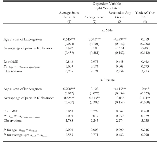
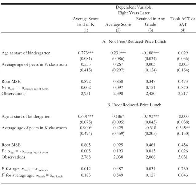
To investigate this possibility, we estimated separate models by gender and free or reduced-price lunch status in kindergarten. We present the TSLS estimates by gender in Table 5 and by free lunch status in Table 6. The estimates suggest that being relatively old may have a greater benefit for boys than for girls and for higher-income children than for lower-income children. In particular, the positive effects of more mature peers tend to be larger and more often statistically significant for girls – particularly for test scores and the ACT/SAT taking rate (Table 5, Panel B) – and for children receiving free or reduced-price lunch (Table 6, Panel B). The difference in TSLS coefficients on between lower-income and higher-income children is starker than that between boys and girls, and in the case of taking the ACT or SAT, it is in fact statistically significant.
While the estimates are somewhat too imprecise to draw strong conclusions, they are consistent with the existence of a relative age effect. Yet, even for these boys and higher-income children, the net effect of exposure to more mature peers is positive.
t 2
VII. Conclusion
In this paper, we have estimated the net effects of having more mature peers – and being young relative to one’s peers – using data from an experiment where children of the same biological age were randomly assigned to different classrooms at the start of school. We find that children who were young relative to their kindergarten classmates generally performed no worse on achievement tests, were no more likely to be retained, and were no less likely to take the ACT or SAT. In fact, having more mature classmates appears to have made the average child better off, consistent with the broader peer effects literature
documenting the positive spillovers from having higher-scoring peers. We arrive at similar conclusions when we use a child’s kindergarten schoolmates as a peer group, but the estimates are less precise. The benefits of having older peers also appear to be weaker for boys and higher-income children, consistent with the existence of larger relative age effects – and the higher incidence of delay – among these groups.
These findings suggest the reduced-form age effects that have frequently been estimated in the literature on school entry age are better interpreted as absolute age effects than relative age effects. In other words, while our data do not allow us to determine whether the age effects reflect differences in developmental trajectories, age at observation, or true effects of entering school later, there is something about being older in an absolute sense that drives the observed positive impacts. The driving factor does not appear to be being one of the oldest in the classroom.
In practice a parent’s decision to delay a child’s school entry increases his absolute age but exposes him to younger peers, and we cannot conclusively say whether this decision will help or harm him on net. We can conclude, however, that one student’s choice to delay will not harm other children, and may in fact help them.
References
Angrist, Joshua and Jorn-Steffen Pischke. 2009. Mostly Harmless Econometrics: An Empiricist’s Companion. Princeton: Princeton University Press.
Bedard, Kelly and Elizabeth Dhuey. 2006. “The Persistence of Early Childhood Maturity: International Evidence of Long-Run Age Effects.” TheQuarterly Journal of Economics 121(4): 1437-1472.
Bedard, Kelly and Elizabeth Dhuey. 2012. “School Entry Policies and Skill Accumulation Across Directly and Indirectly Affected Men.” Journal of Human Resources 47(3): 643-683.
Black, Sandra, Paul Devereux, and Kjell Salvanes. 2011. “Too Young to Leave the Nest? The Effects of School Starting Age.” Review of Economics and Statistics,93(2): 455-467.. Boozer, Michael A. and Stephen E. Cacciola. 2001. “Inside the ‘Black Box’ of Project STAR:
Estimation of Peer Effects Using Experimental Data.” Yale University Economic Growth Center Working Paper 832.
Carrell, Scott and Mark Hoekstra. 2010. “Externalities in the Classroom: How Children Exposed to Domestic Violence Affect Everyone’s Kids.” American Economic Journal: Applied Economics 2(1): 211-228.
Cascio, Elizabeth U. and Ethan G. Lewis. 2006. “Schooling and the Armed Forces Qualifying Test: Evidence from School Entry Laws,” The Journal of Human Resources 41(2): 294-318.
Chetty Raj, John N. Friedman, Nathaniel Hilger, Emmanuel Saez, Diane Schanzenbach, and Danny Yagan. 2011. “How Does Your Kindergarten Classroom Affect Your Earnings? Evidence from Project STAR.” Quarterly Journal of Economics 126(4): 1593-1660.
Datar, Ashlesha. 2006. “Does Delaying Kindergarten Entrance Give Children a Head Start?” Economics of Education Review 25: 43-62.
Dee, Thomas S. 2004. “Teachers, Race, and Student Achievement in a Randomized Experiment.” The Review of Economics and Statistics 86, 195-210.
Dee, Thomas S. and Benjamin J. Keys. 2004. “Does Merit Pay Reward Good Teachers? Evidence from a Randomized Experiment.” Journal of Policy Analysis and Management 23(3): 471-488.
Ding, Weili and Steven F. Lehrer. 2007. “Do Peers Affect Student Achievement in China’s Secondary Schools?” Review of Economics and Statistics 89(2): 300-312.
Dobkin, Carlos and Fernando Ferreira. 2010. “Do School Entry Laws Affect Educational Attainment and Labor Market Outcomes?” Economics of Education Review 29(1): 40-54.
Duflo, Esther, Pascaline Dupas and Michael Kremer. 2011. “Peer Effects, Teacher
Incentives, and the Impact of Tracking: Evidence from a Randomized Evaluation in Kenya.” American Economic Review 101: 1739-1774.
Elder, Todd E. and Darren H. Lubotsky. 2009. “Kindergarten Entrance Age and Children’s Achievement: Impacts of State Policies, Family Background, and Peers.” Journal of Human Resources 44(3): 641-683.
Figlio, David. 2007. “Boys Named Sue: Disruptive Students and Their Peers.” Education Finance and Policy 2(4):376-94.
Fredrikksson, Peter and Björn Öckert. 2006. “Is Early Learning Really More Productive? The Effect of School Starting Age on School and Labor Market Performance.” IFAU Working Paper 2006:12. Uppsala: Institute for Labour Market Policy Evaluation.
Gootman, Elissa. 2006. “Preschoolers Grow Older as Parents Seek an Edge.” The New York Times (October 19, 2006).
Gormley, William T. and Ted Gayer. 2005. “Promoting School Readiness in Oklahoma: An Evaluation of Tulsa’s Pre-K Program.” The Journal of Human Resources 40(3): 533-558. Graham, Bryan S. 2008. “Identifying Social Interactions through Conditional Variance
Restrictions.” Econometrica 76(3): 643-660.
Hanushek, Eric A., John F. Kain, Jacob M. Markman and Steven G. Rivkin. 2003. “Does Peer Ability Affect Student Achievement?” Journal of Applied Economics 18: 522-544. Krueger, Alan B. 1999. “Experimental Estimates of Education Production Functions,” The
Quarterly Journal of Economics 114(2): 497-532.
Krueger, Alan B. and Diane M. Whitmore. 2001. “The Effect of Attending a Small Class in the Early Grades on College Test-Taking and Middle School Test Results: Evidence from Project STAR,” TheEconomic Journal 111: 1-28.
Kugler, Adriana, Scott Imberman, and Bruce Sacerdote. 2012. “Katrina’s Children: Evidence on the Structure of Peer Effects from Hurricane Evacuees.” American Economic Review, forthcoming.
Lavy, Victor, M. Daniele Paserman, and Analia Schlosser. 2012. “Inside the Black Box of Ability Peer Effects: Evidence from Variation in the Proportion of Low Achievers in the Classroom.” The Economic Journal 122(559): 208-237.
McCrary, Justin and Heather Royer. 2011. “The Effect of Maternal Education on Fertility and Infant Health: Evidence from School Entry Policies Using Exact Date of Birth.” American Economic Review 101(1): 158-195.
McEwan, Patrick and Joseph Shapiro. 2008. “The Benefits of Delayed Primary School Enrollment: Discontinuity Estimates using Exact Birth Dates.” The Journal of Human Resources 43(1): 1-29.
Puhani, Patrick A. and Andrea M. Weber. 2005. “Does the Early Bird Catch the Worm? Instrumental Variable Estimates of Educational Effects of Age at School Entry in Germany.” IZA Discussion Paper 2005. Bonn: Institute for the Study of Labor. Sacerdote, Bruce. 2011. “Peer Effects in Education: How Might They Work, How Big are
They, and How Much Do We Know Thus Far?” in Hanushek, Eric A., Stephen Machin and Ludger Woessman, eds., Handbook of the Economics of Education, North Holland: Elsevier.
Schanzenbach, Diane Whitmore. 2006. “Classroom Gender Composition and Student Achievement: Evidence from a Randomized Experiment.” Mimeo, University of Chicago.
Schanzenbach, Diane Whitmore. 2007. “What Have Researchers Learned From Project STAR?” Brookings Papers on EducationPolicy, 2006/07, pp. 205-228.
Weil, Elizabeth. 2007. “When Should a Kid Start Kindergarten?” The New York Times Magazine. (June 3, 2007).
West, Jerry, Anne Meek, and David Hurst. 2000. “Children Who Enter Kindergarten Late or Repeat Kindergarten: Their Characteristics and Later School Performance.” NCES 2000-039. Washington, D.C.: U.S. Department of Education.
Whitmore, Diane M. 2005. “Resource and Peer Impacts on Girls’ Academic Achievement: Evidence from a Randomized Experiment,” American Economic Review 95(2):199-203.
Notes: Figure plots the age at which Project STAR participants born on each day of the calendar year would have been expected to enter kindergarten, given Tennessee’s regulation that entering
kindergartners must be aged five by September 30 (darkened circles). Figure also plots the average age of Project STAR participants on September 1, 1985 (hollow circles).
4.9 5.15 5.4 5.65 5.9 6.15
Jan 1 Apr 1 Aug 1 Oct 1 Dec 31
Birthday expected entry age average entry age
Project STAR Kindergarten Cohort
Mean
Standard
deviation N
(1) (2) (3)
A. Age variables
Expected age at the start of kindergarten 5.38 0.28 6248 Age in at the start of kindergarten 5.43 0.35 6248 Average expected age of kindergarten classmates 5.38 0.07 6248 Average age of kindergarten classmates 5.43 0.09 6248 B. Demographic/SES variables
Female 0.49 - 6248
Black 0.33 - 6248
Free/reduced-price lunch (in kindergarten) 0.49 - 6248 C. Other characteristics of kindergarten classmates
Fraction Female 0.49 0.12 6248
Fraction Black 0.33 0.41 6248
Fraction Free/Reduced-Price Lunch (in K) 0.49 0.28 6248 D. Kindergarten teacher characteristics
Black 0.17 - 6248
Has MA 0.35 - 6248
Has <2 Years Experience 0.10 - 6248
E. Kindergarten class characteristics
Small 0.30 - 6248
Regular with Aide 0.35 - 6248
F. Outcome variables
Standardardized test score, end of kindergarten 0.00 1.00 5719 Standardardized test score, 8 years later 0.12 0.99 4436
Ever retained, 8 years later 0.25 - 4508
Took ACT/SAT 0.47 - 6248
Table 1 - Descriptive Statistics for Project STAR Kindergarten Cohort
Notes: Sample includes individuals with non-missing demographic/SES variables, kindergarten classmate characteristics, kindergarten teacher characteristics, and kindergarten class characteristics. See text for more details.
Expected age at start of K Expected average age of K classmates P on joint significance Dependent variable: (1) (2) (3) Demographic/SES variables Female 0.013 -0.013 0.826 (0.022) (0.095) Black 0.007 0.019 0.732 (0.010) (0.041)
Free/reduced-price lunch (in kindergarten) -0.054 *** -0.077 0.018 (0.019) (0.092)
Other characteristics of kindergarten classmates
Fraction female -0.002 -0.024 0.878
(0.005) (0.091)
Fraction black 0.001 0.02 0.885
(0.002) (0.040)
Fraction free/reduced-price lunch (in kindergarten) -0.004 -0.127 0.028 (0.005) (0.091)
Kindergarten teacher characteristics
Black -0.018 -0.315 0.096
(0.012) (0.220)
Has MA -0.016 -0.303 0.616
(0.019) (0.352)
Has <2 years experience -0.003 -0.047 0.781 (0.015) (0.274)
Kindergarten class characteristics
Small 0.032 0.562 0.226
(0.024) (0.440)
Regular with aide 0.009 0.127 0.296
(0.024) (0.435) Coefficient (standard error) on: Table 2a - Predictive Power of Instrumental Variables for Background Characteristics
Notes: Each row represents a different regression. All regressions are based on 6248 observations and include school fixed effects. Standard errors are clustered on kindergarten classroom. ***, **, and * represent statistical significance at the 1%, 5%, and 10% levels, respectively.
Expected age at start of K Expected average age of K classmates P on joint significance Dependent variable is dummy=1 if observed: (1) (2) (3) Standardardized test score, end of kindergarten 0.009 0.073 0.376
(0.012) (0.061)
Standardardized test score, 8 years later 0.031 -0.033 0.293 (0.020) (0.075)
Ever retained, 8 years later 0.031 -0.019 0.297 (0.020) (0.075)
Coefficient (standard error) on:
Table 2b - Predictive Power of Instrumental Variables for Observation of Dependent Variables
Notes: Each row represents a different regression. All regressions are based on 6248 observations and include school fixed effects. Standard errors are clustered on kindergarten classroom. ***, **, and * represent statistical significance at the 1%, 5%, and 10% levels, respectively.
(1) (2) (3) (4) (5)
Age at start of kindergarten 0.242*** 0.244*** 0.283*** 0.250*** 0.277*** (0.038) (0.039) (0.037) (0.045) (0.038) Average age of peers:
in kindergarten classroom 0.178 0.112 (0.267) (0.251)
in kindergarten school cohort 0.907 -0.258 (0.871) (0.767)
R-squared 0.23 0.23 0.30 0.01 0.12
Root MSE 0.885 0.885 0.844 0.997 0.942
P: αage = - αaverage age of peers 0.129 0.133 0.194 0.981
Age at start of kindergarten 0.707*** 0.716*** 0.683*** 0.732*** 0.699*** (0.057) (0.058) (0.055) (0.061) (0.057) Average age of peers:
in kindergarten classroom 0.847** 0.724* (0.407) (0.374)
in kindergarten school cohort 2.538* 2.314 (1.351) (1.531)
Root MSE 0.900 0.901 0.856 1.017 0.963
P: αage = - αaverage age of peers 0.0003 0.0004 0.021 0.057
Observations 5,719 5,719 5,719 5,719 5,719
Controls‡? N N Y N Y
School fixed effects? Y Y Y N N
B. Two-Stage Least Squares† Table 3 - Estimated Effects of Entry Age and Peer Average Entry Age on
Average Test Score, End of K (Standardized) Dependent Variable:
A. Ordinary Least Squares Test Scores at the End of Kindergarten
Notes: Each column and panel of the table presents estimates from a different regression. The dependent variable in all regressions is the standardized average of reading and math Stanford Achievement Test scores at the end of kindergarten. Standard errors (in parentheses) are clustered on kindergarten classroom in columns 1 to 3 and on school attended in kindergarten in columns 4 and 5. ***, **, and * represent statistical significance at the 1%, 5%, and 10% levels, respectively.
† The instrument for a child's age at the start of kindergarten is his expected age given his birthday and the September 30th kindergarten entry cutoff birthdate in Tennessee. The instrument for the average age of child's peers is their average expected age.
‡ Dummies for whether child is female, black, or received free/reduced-price lunch in K; fractions of K classmates with these characteristics; whether the kindergarten teacher is black, has an MA, or has 0 to 1 years of experience; and dummies for whether kindergarten class is small or regular sized with teacher's aide. The specifications in column 5 also include the fractions of a child's schoolmates in kindergarten who were female, black, or received free or reduced-price lunch.
Average Score Retained in Any Grade Took ACT or SAT (1) (2) (3)
Age at start of kindergarten 0.221 *** -0.191 *** 0.004 (0.065) (0.026) (0.024) Average age of peers in K classroom 0.430 * -0.136 0.172
(0.248) (0.115) (0.106)
Root MSE 0.890 0.405 0.465
P: αage = - αaverage age of peers 0.010 0.006 0.103
Age at start of kindergarten 0.225*** -0.192*** 0.004 (0.069) (0.025) (0.027) Average age of peers in K school cohort 0.789 -0.459 0.205
(0.630) (0.316) (0.279)
Root MSE 0.902 0.413 0.469
P: αage = - αaverage age of peers 0.116 0.0431 0.456
Observations 4,436 4,508 6,248
Dependent Variable:
B. Entry Age + School Level Peer Effect A. Entry Age + Classroom Level Peer Effect Table 4 - TSLS Estimates of the Effects of Entry Age and Peer Average Entry Age on Later
Outcomes
Eight Years Later:
Notes: Each column and panel of the table presents estimates from a different regression. All models are estimated using two-stage least squares. The specification in Panel A is the same as that in Table 3 column 3. The specification in Panel B is the same as that in Table 3 column 5. Standard errors (in parentheses) are clustered on kindergarten classroom in Panel A and on school attended in kindergarten in Panel B. ***, **, and * represent statistical significance at the 1%, 5%, and 10% levels, respectively.
Average Score
End of K Average Score
Retained in Any Grade
Took ACT or SAT
(1) (2) (3) (4)
Age at start of kindergarten 0.645*** 0.343*** -0.279*** 0.059 (0.073) (0.101) (0.042) (0.038) Average age of peers in K classroom 0.627 0.190 -0.154 -0.003 (0.459) (0.381) (0.162) (0.142)
Root MSE 0.843 0.978 0.445 0.463
P: αage = - αaverage age of peers 0.009 0.174 0.009 0.693
Observations 2,936 2,191 2,234 3,213
Age at start of kindergarten 0.708*** 0.122 -0.115*** -0.048 (0.077) (0.075) (0.034) (0.033) Average age of peers in K classroom 0.824** 0.613** -0.062 0.331** (0.407) (0.308) (0.152) (0.160)
Root MSE 0.868 0.799 0.362 0.468
P: αage = - αaverage age of peers 0.000 0.019 0.250 0.079
Observations 2,783 2,245 2,274 3,035
P for age: αmale = αfemale 0.000 0.007 0.000 0.046
P for average age: αmale = αfemale 0.586 0.771 0.482 0.290
Table 5 - TSLS Estimates of the Effects of Entry Age and Peer Average Entry Age, by Gender
Eight Years Later: Dependent Variable:
A. Male
B. Female
Notes: Each column and panel of the table presents estimates from a different regression. All models are estimated using two-stage least squares and are based on the specification presented in Table 3, column 3. Standard errors (in parentheses) are clustered on kindergarten classroom. ***, **, and * represent statistical significance at the 1%, 5%, and 10% levels, respectively.