Vector Autoregressive Models for Multivariate Time Series Analysis; Macroeconomic Indicators in Ghana

Vector Autoregressive Models for Multivariate Time Series

Analysis; Macroeconomic Indicators in Ghana

Erasmus Tetteh-Bator 1*, Mohammed Adjei Adjieteh 12, Lin Chun Jin 3, Theophilus Quachie Asenso4 1, 3 _{College of Science, Hohai University, No. 1 Xikang Road, 211100, Nanjing, China.}

2

School of Finance, Shanghai University of Finance and Economics, No.777 Guoding Road, Shanghai, 200433, China.

4_{African Institute for Mathematical Sciences (AIMS), Cameroon.} * E-mail of the corresponding author: [email protected]

Abstract

This study investigated the relationship, the percentage contribution of endogenous shocks and the direction of causality between real gross domestic product, exchange rate, foreign direct investment and unemployment rate in Ghana. It employed the multivariate Johansen co-integration test via vector auto-regressive model and the vector error correction model, to examine both long-run and short-run dynamic relationships respectively, between the selected macroeconomic variables for the period 1991-2016. The dynamic interactions between the variables were studied with Granger causality tests, impulse response functions, and forecast error variance decompositions. Augmented Dickey-Fuller (ADF) test indicated that all the variables were stationary after their first differencing, thus variables are integrated of order one, I (1). The diagnostic tests on the model residuals revealed that the models were adequate, valid and stable. The Trace test statistic of the Johansen cointegration test indicated one cointegrating relationship indicating long run relationship among the variables. Granger Causality analysis indicated a uni–directional causal relationship between real GDP and FDI. It also showed that FDI Granger-causes all of the other variables. The results revealed the positive effect and sensitivity of the FDI variable in determining the activities pertaining to real GDP, exchange rate, and unemployment rate and vice versa in the Ghanaian economy.

Keywords: Vector Autoregression Model (VAR), Multivariate Time Series, Macroeconomic Variables, Cointegration, Granger causality, Impulse response function, Forecast error variance decomposition,

Abstract

1. Introduction

Countries all over the world, in spite of their history, geographical location or political status aims to achieve and maintain high economic growth coupled with low or high values of major macroeconomic variables such as real GDP, inflation, exchange rates, FDI, stock prices, unemployment rate among others to influence growth and development of the country. (Maghayereh, 2002).

Gross domestic product (GDP) refers to the value of all final goods and services produced within a country or an area during a time period. It is often considered the best standard of measuring national economic conditions

(Mankiw & Taylor 2007). GDP is the primary indicator which is used to check the financial health status of a country as a whole and GDP per capita is often combined with measures of the purchasing power parity (PPP) to measure people’s living standard more objectively (Larsson & Harrtell, 2007). GDP Growth Rate in Ghana averaged 1.98 percent from 2006 until 2016, reaching an all-time high of 8.10 percent in the first quarter of 2012 and a record low of -2.20 percent in the fourth quarter of 2008. Exchange rate also known as Foreign exchange rate or Forex rate between two currencies is the price of one currency in terms of another. Exchange rate is the value of a foreign nation currency in terms of the home nation’s currency. Exchange rates are important economic indicators that affect the relative price of domestic and foreign goods. The dollar price of Ghana goods to an American is determined by the interaction of two factors, the price of Ghana goods in cedis and the cedi/dollar exchange rate. Many researchers attribute exchange rate volatility to the fact that, it is empirically difficult to predict future exchange rate values (Killian and Taylor, 2001; Taylor, J., 2001).

Foreign direct investment (FDI) is an investment made by a company or individual in one country, whose business interests is in another country, in the form of either establishing business operations or acquiring business assets in the other country, such as ownership or controlling interest in a foreign company. FDI is an

essential catalyst for economic growth, it is carried out in order to take advantages of cheaper wages such as tax exemptions as incentives to entre free access markets of a country. The benefits of FDI have driven numerous countries, especially developing countries such as Ghana to increase their FDI inflows. In Ghana, stock of FDI stood at USD 319 million in 1990 but grew to USD 1,554 million in 2000 representing 387% growth over a decade. In 2013, it increased further to USD 19,848 million representing 1,177% growth between 2000 and 2013. However, between 2008 and 2013 FDI inflows to Ghana increased by 164.4%, moving from USD 1,220 million in 2008 to USD 3,226 million in 2013 (UNCTAD, 2014).

The unemployment rate is the share of the labour force over a country’s population that is jobless, expressed as a percentage. Unemployment rate is a lagging indicator, which implies that it rises or falls in the state of changing economic conditions, rather than anticipating them. When the economy is in recession and jobs are scarce, the unemployment rate of a country can be expected to rise while when the economy is boomed at a growing rate and jobs are relatively enough, the rate can be expected to fall. A decline in employment elasticity of output in Ghana has been recorded over the years. Ghana still battles with high incidence of unemployment, thus joblessness and job-seeking causing higher unemployment rate particularly in recent times. This suggest failure in socio-political and economic policy implications and the underutilization of both human and natural resources in the country. (William Baah‐Boateng, 2014).

VAR model is useful for describing the dynamic behaviour of economic and financial time series and for forecasting. The reason for which this model has become of great importance and gained popularity, is with the realization of relationships among financial variables that are so complex, that traditional time-series models have failed to fully capture. VAR models treat all variables as a prior endogenous.

A lot of researches have been carried out all over the world to find interaction relationship between major macroeconomic indicators. For instance, Agalega et al (2013) considered two variables to establish their relationship with GDP of Ghana, they concluded that there exist a positive relationship between GDP and inflation rate given the data for the period under consideration. In addition, Olaiya et al. (2012) used a tri-variate vector error correction model and the Johansen & Juselius co-integration approach to study the relationships among inflation, government expenditure and economic growth in Nigeria. It confirmed a negative co-integration relationship between inflation and growth and unidirectional causality running from economic growth to inflation. Altaf et al. (2012) determined the significance of macroeconomic variables on Pakistan’s economic growth with the application of VAR modelling using annual time series data. Their quantitative evidence showed that real per-capita income growth is caused by money-supply. In this research, the interest is to model GDP and the interaction between selected economic indicators (real gross domestic product, exchange rate, foreign direct investment, and unemployment rate) in Ghana with the approach of vector Auto-regressive (VAR) over time period from (1991 - 2016) in Ghana.

2. Material and Methods

2.1 Data Collection Technique

The study was carried out using secondary macroeconomic time series data on annual basis from 1991 to 2016.The data was obtained from the Bank of Ghana database, World Bank database, and International labour organization (ILOSTAT) database. Other augmenting sources of this study will include published articles and journals, working papers, textbooks and relevant internet resources.

2.2 Unit Root Test

Unit root test was conducted in order to investigate the stationarity properties of the time series and the Augmented Dickey Fuller (ADF) test was applied to all variables in level and in first difference in order to formally establish their order of integration. ADF unit root test, the null hypothesis of interest is

H

O

:





0

(the series contains unit root or is non-stationary) against the alternative

H

₁

:



0

(the series contains no unit root or is stationary). All statistical tests were controlled at 5% significance level (α). If p-value of the ADF test is less than critical value (α value), we reject the null hypothesis, then the data is stationary. The ADF regression test is as follows: 1 1 1 p t t t i t t i Y

  

Y



Y



     



  1

Where is a constant (intercept),_t the coefficient on time trend series, ₁ 1 p i t i Y    



is the sum of the lagged values of the dependent variable Y_tand p is the lag order of the autoregressive process. The parameter of interest in the ADF test is.

2.3 Model Specification

According to Sims (1980), Vector Auto regression (VAR) model is considered as a valuable tool in investigating the dynamic effects of two or more given variable on one another. The VAR model expresses the current value of an endogenous variable as a function of deterministic terms and the lagged values of the endogenous variables. According to Bardsen & Lutkepohl (2011), if there is a Co-integration relationship among the variables, the analysis of such process is easily done with a model called Vector Error Correction Model (VECM).

2.4 Model Selection Criteria

Standard lag order selection criteria was used as a guide in determining the optimal number of lags to be employed in estimating the VAR for the analysis such that the residuals are not serially correlated. The choice of the lag order selection criterion was significant in implications the accuracy of the VAR impulse response functions. (Ivanov & Kilian, 2005). The multivariate case with n variables, T observations, a constant term and a maximal lag of p, these criteria are as follows:

Final prediction error (FPE)

 

1

 

1 K T np FPE p p T kp     _{ }      2

Akaike’s information criterion (Akaike (1973, 1974))

 

 

2 2

AIC p In p pn

T

   3

Hannan-Quin criterion (Hannan & Quin (1979), Quin (1980)

 

 

2InInT 2

HQ p In p pn

T

   4

Schwarz information criterion (SIC) (Schwarz (1978)

_{SC p}

 

_In

 

_p InT _pn2 T

   5

the choice of the best model was based on the model selection criteria, the minimum model selection criteria compared to others, the model with the minimum values of Akaike Information Criterion (AIC), and Schwarz Bayesian Information Criterion (SBIC) was adjudged the best model.

2.4 Model Diagnostic

The diagnostic stage involved checking whether the selected model adequately represents a fitted model appropriate for use. The diagnostic tests were run on both the VAR and VECM model to check their validity before the model draws any meaningful conclusion or make generalization. The study used the Breusch-Godfrey- LM tests to check for residual auto-correlation and also Lagrange-multiplier test to investigate a possible serial correlation in the error term. It employed the Skweness/Kurtosis test for testing normality of the series and the Roots of Characteristic Polynomial was used to check the stability of the estimated parameters in the model over model time.

2.5 Vector Autoregressive (VAR) model and Vector Error Correction Model (VECM)

When co-integration is being detected between series by the VAR model, we know that there exist a long-term equilibrium relationship between the non-stationary series but in the short run, there may be disequilibrium. The

next step is to specify and estimate a vector error correction model (VECM) including the error correction term to investigate dynamic behavior of the model and evaluate the short-run properties of the co-integrated series. The size of the error correction term indicates the speed of adjustment of any disequilibrium towards a long-run equilibrium state (Engle & Granger, 1987).

A VAR of order p: 1 0 1 p t i t t t i Y



Y



X

 

 



   6

Where

y

_t is a k-vector of non-stationary I (1) variables,

X

_t is a d-vector of deterministic variables, and

i

  are matrices of coefficients,



_t is a vector of independent and identically distributed innovations, 0

 is a (n*1) of constants, P is the number of lags.

If the endogenous variables are each I(1) we can write the VAR(p) model as a vector error correction model (VECM): The Vector Error Correction Model (VECM) is given as:

1 0 1 1 1 p t i t t t t i Y



r Y Y X



      



      7

Where Δ is the first difference operator and



_t is the white noise term

1 p i j j i r     



and 1 p i i



  



  are square matrices whose elements depend on the coefficients of long run model and Yt contains the

endogenous variables of the model. The  is a g x g matrix containing the long-run parameter, If there are r co-integration vectors, then  can be expressed as a product of two matrices as 



where both_and 𝛽

are a x r matrices. The matrix 𝛽 contains the coefficients of long-run relationship and  contains the speed of adjustment parameters which are also interpreted as the weight with which each co-integration vector appears in a given equation.

2.6 Cointegration Test: The Johansen Approach

Johansen’s approach to co-integration was used to determine the number of co-integrating link between the selected macroeconomic variables as well as providing estimates of these vectors. Co-integration transforms the linear combination of two non-stationary time series into a stationary one. This means that when co-integrating relationships exists between variables, then that implies, they share similar stochastic trends and hence a long run relationship exists between them. The Two different likelihood ratio tests developed by Johansen for testing the number of co-integration vectors (r): thus, the order or rank of co-integration (r) are the trace test and the maximum eigenvalue test.

The test statistics for the trace test and maximum eigenvalue test are as follows:

 





1 1 n trace i i r r T In      



 8









max r r, 1 TIn 1 i 1     _ 9

Wherer1, 2,...,n T is the sample size, n is number of endogenous variables and i is the largest

eigenvalue.

2.7 Granger Causality Analysis,Impulse Response Function and Variance Decomposition Analysis

Granger causality was used to measure whether current and past values of a variable help to forecast future values of another variable. In other words, the rationale for granger causality test is to find out if lagged values of a particular variable add any information to forecasting the endogenous variable. By Granger’s representation theorem, if variables are co-integrated, there must be causality in at least one direction and the long run

relationship is free of spurious correlations. Granger (1988) posits two cardinal principles namely the cause precedes the effect. Similarly, if there is an instantaneous causality from to then, the present and past values of predict present value of Also a causality from to is in one direction and it referred to as uni-directional causality while if Granger causes and Granger causes , it is referred to as bi-directional or feedback causality ( ↔ ). The Granger causality test for analysing linear causality relationship between the variables performed by estimating equations of the following form: Compare the unrestricted models; 1 2 1 1 1 1 1 1 1 1 m m t i t i j t i j y   y_  y_ e     



 



  10

With the restricted models;

1 2 2 2 1 2 1 2 1 1 m m t i t i j t i j x   x_  x_ e     



 



  11

Where



x

_t and



y

_t are the first order forward differences of the variables, 𝛼, 𝛽, 𝛳 are the parameters to be estimated and

e

₁,

e

₂ are standard random errors. The lag order m are the optimal lag orders chosen by information criteria.

Impulse Response Function (IRF) was tested to confirm the granger causality test, indicating the extent to which the exogenous random shock can cause short run or long run changes in the respective variables The impulse response function traces the effect of each shock on each variable in the VAR over a given time horizon. It indicates the behavior of variables in response to the various random shocks in the other variables of the model. The empirical evidence on impulse response function will enable the policy maker to predict the consequences of these unanticipated shocks in advance so that they will be well prepared to react to these changes in future. Cholesky adjusted model type of contemporaneous identifying restrictions are employed to draw a meaningful interpretation.

Forecast error variance decomposition was conducted to examine the percentage contribution of shocks emanating from each endogenous variable on itself and also on other endogenous variables. Variance decomposition determined how much of the forecast error variance of each of the variable can be explained by endogenous shocks to the other variables. This analysis was employed as an additional evidence presenting more detailed information regarding the variance relations among the selected macroeconomic variables.

3. Results and Discussion

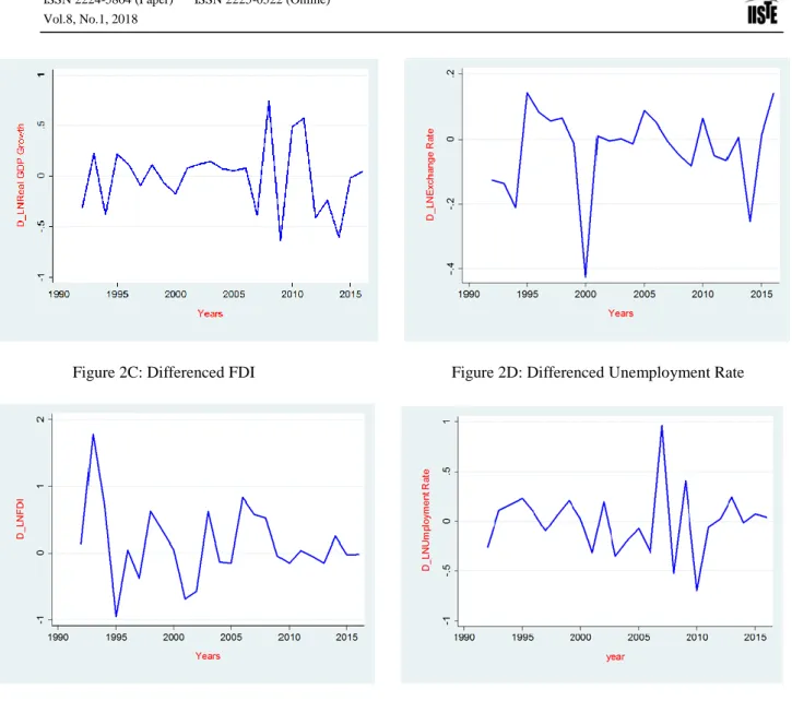
Figures 2A, 2B, 2C and 2D are Time Series Plots of first Differenced real GDP, exchange rates, FDI and unemployment rate respectively in Ghana during the sample period of 1991 to 2016. It can be confirmed that the variables are stationary after the first difference from the various figures since the variables tended to fluctuate more around their means.

Table 1, presents the results of the unit root testing of variables at level using the ADF tests. The result indicates that all the data of the variables are non-stationary at levels since the variable’s p-value of the ADF test is greater than the significance level of 5%, so we fail to reject the null hypothesis of unit root and claim that the series is non-stationary. Table 2 presents the result of the unit root testing of variables at first difference using the ADF tests. The result indicates that all the data of the variables are stationary at first difference since the absolute value of the test statistic of the variable is greater than the absolute value of the critical value, hence we to reject the null hypothesis and claim that the series is stationary. It is therefore clear that all the variables in each of the series is integrated of order one (thus, each series is I (1)) and this estimation process eliminates the possibility of spurious regression. Achieving stationarity is a pre-condition for estimating the VAR model and consequently cointegration analysis.

That lag length selection determines which year selection would have significance on the current results and its chosen based on five different lag selection criterions. In table 3, a majority of four criterion chose lag one as the number of parameters which minimizes the value of the information criteria.

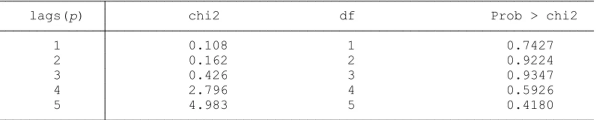
The result of Table 4 shows that, the null hypothesis of no serial autocorrelation failed to be rejected, for the Breusch-Godfrey LM test for all lags, since their p-values are greater than the significance level of 5% and we conclude that there is no serial autocorrelation in the residuals of the model. The ARCH LM test results, failed to reject the null hypothesis of no ARCH effect in the residuals of the selected model and conclude that there is no

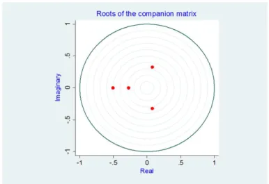
heteroscedasticity in the model residuals since majority of p-values are all greater than the alpha (α) value of 0.05. Table 5 shows that, in the Skewness/Kurtosis test for normality, the null hypothesis is rejected for all residuals which indicate that, all residuals are normally distributed since the p-values of Skewness, Kurtosis and Joint are all greater than the 5% significance level. The inverse roots of the AR characteristics polynomials lie within the unit circle. This indicates that there was no problem in terms of stability of one-lag VAR model for both the base and extended models. The roots of characteristics polynomial do not lie outside the unit circle as show in figure 1 and table 6. From the analysis, VAR (1) satisfies the stability condition. Hence the VAR model is adequate. The same tests and results of no serial autocorrelation, no heteroskedasticity, and stability of the VECM Residuals in the vector error correction model was revealed. These results validate the adequacy of the VECM model.

At 5% level of significance, table 7 shows Trace test statistic of the Johansen cointegration. There is one cointegrating relationship among the variables. Specifically, the null hypothesis of no cointegrating relationship is rejected since the computed value of the trace statistic of 52.2746 is greater than it critical value of 47.21. Hence, we conclude that at least there exist a stable long run relationship the selected macroeconomic variables. Table 8 also shows the long run relationship among the selected macroeconomic variables. The model for the long-run cointegrating relationship between exchange rate, FDI, Unemployment and real GDP is modelled as follows:

GDP 0.249075 6.247496 1.545772

0.8316895

InR InExrate InFDI

InUnemprate

      

  6

The coefficients of FDI and Unemployment rate are positively signed. Exchange Rate, on the other hand, has a negative sign. The positive sign indicates a positive association between the variable and Real GDP. An increase in the variable will turn to increase the value in Real GDP and vice versa. Also, the negative sign indicates a negative association between the variable and Real GDP. An increase in the variable will cause a reduction in the value in Real GDP and vice versa.

The error correction term indicates the rate at which the disequilibrium between the long-run and the short-run estimates are corrected for. The vector error correction model results show that the model has AIC of 2.962225, HQIC of 3.454576 and SBIC of 5.094717. The sign and magnitude of these error correction parameters give information about the direction and speed of adjustment towards the long run equilibrium course. The result for the first equation, the Real GDP equation in the VECM indicates that, the coefficient of the error correction terms ecm1t-1 of real GDP is 0.18825635. Thus, on annual basis, 0.1883% of the disequilibrium between the long-run and short-run estimates are corrected and brought back to equilibrium. The error correction term is not correctly signed and statistically insignificant at 5% significant level. The exchange rate equation in the VECM indicates that, the coefficient of the error correction terms ecm1t-1 of exchange rate is 0.1152735. The error correction term is not correctly signed and statistically insignificant at 5% significant level. The FDI equation in the VECM indicates that the coefficient of the error correction terms ecm1t-1 of exchange rate is -0.7783414. The error correction term is correctly signed and statistically significant at 5% significant level. The unemployment rate equation in the VECM indicates that the coefficient of the error correction terms ecm1t-1 of unemployment is -0.0022176. The error correction term is correctly signed but statistically insignificant at five percent level. The results are shown in table 9.

Table 10 presents the result for the granger causality analysis between the variables (if any) and the direction of causality of the systems. The estimate shows that at 5% significance level, FDI Granger-causes all of the variables; real GDP, exchange rate, and unemployment rate. Thus, the past values of FDI can be used to predict future values of each of the other variables in Ghana. Also, Unemployment rate granger causes FDI, and this finding implies that there is a bidirectional causality between FDI and Unemployment rate in Ghana. However, real GDP does not granger causes any of the other variables and thus past Real GDP cannot be used to predict their future values. Hence there is a unidirectional causality between FDI and real GDP. Also, exchange rate does not granger causes unemployment rate and vice versa in Ghana.

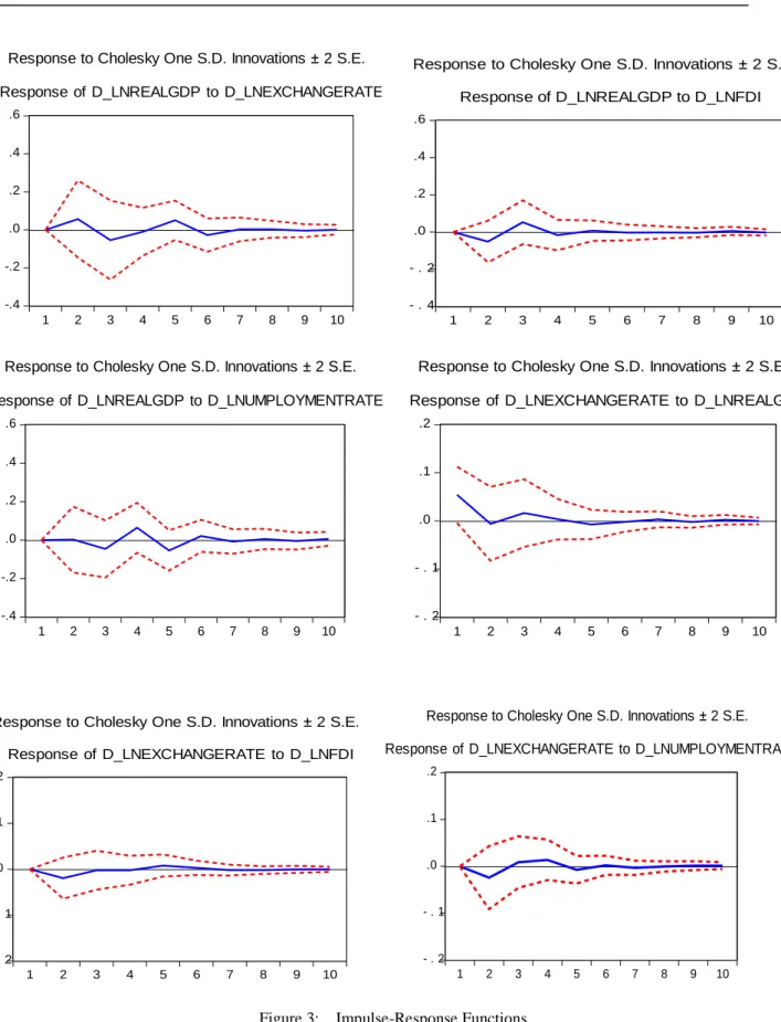
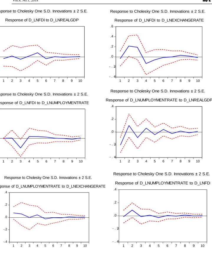
Figure 3 shows the generalized impulse response functions, which trace the effects of a shock from one endogenous variable onto the other variables in the system. It should be noted that, a shock to one variable does affect itself and other endogenous variables in the system due to the dynamic lag structure. A unit shock of Real GDP to FDI rate creates a slight fluctuation and dies off with the reaction remaining positive, this confirms the unidirectional causality between real GDP and FDI. A unit shock of real GDP to Unemployment rate initially creates a positive reaction, in the second year, the reaction becomes negative. From 3 to 5 years, the reaction becomes positive again and after 5 years, reactions will remain steady and positive. A unit shock of Exchange

rate to any of the variables; real GDP, FDI and Unemployment rate has a slight fluctuation in its initial 1 to 5 years and after 5 years, it slowly dies off, with all reactions remaining positive. A unit shock of FDI to real GDP creates a slight fluctuation initially and the reaction was negative over 3 years. After 3 years, reaction becomes positive after a strong fluctuation. After 7 years, the reaction becomes steady and remained positive. A unit shock of FDI to Exchange rate creates a strong fluctuation and the reaction is positive for three and half years. The reaction is negative from three and half years to 6 years and after 7 years, there is a slight fluctuation and the reaction becomes positive again. A unit shock of FDI to Unemployment rate creates an initial strong fluctuation in 4 years and the reaction is negative. After 4 years the reaction becomes positive with a slight fluctuation and remains positive till the end. A unit shock of Unemployment rate to FDI creates a strong fluctuation in the initial stage within the first 5 years and the reaction remains steady and positive till the end. This confirms the bidirectional causality between Unemployment rate and FDI.

Variance decomposition results of Real GDP shows that with time, the effect of exchange rates, FDI and unemployment rate increases. Variance decomposition results of Exchange rate shows that with time, the effect of all variable increases the forecast error variance of Exchange rate, with FDI being least contributor and real GDP as the most effective variable. This suggests that, shock of real GDP has a positive effect of the forecast error variance of the Exchange rate. Variance decomposition of FDI results implies that with time, the effect of all variable increases with the forecast error variance of FDI, with real GDP being least contributor and Exchange rate as the most effective variable. This suggests that FDI is hugely influenced by Exchange rate and Unemployment rate. This result confirms the unidirectional causality between FDI and Exchange rate and the bidirectional causality between FDI and Unemployment rate respectively. Variance decomposition results of Unemployment rate suggests that Unemployment rate is hugely influenced by real GDP, followed by a slight percentage explained by Exchange rate and FDI, which confirms the bidirectional causality between Unemployment rate and FDI.

4. Conclusion

The study revealed the existence of a long run equilibrium relationship between real GDP growth, exchange rates, FDI and unemployment rate. These findings suggest that, the positive contribution of FDI to Ghana’s GDP and economic growth is about, 1.545772 with significant contribution in the growth model. However, exchange rate has a negative contribution and a significant contribution in the growth model too. The result of the Granger causality analysis shows there exist causality between variables. In the short-term relationships, the findings revealed unidirectional causality between real GDP growth rate and FDI, as well as a bidirectional causality between FDI and unemployment rate thus, the two variables can each be used as a predictor of the other. While FDI granger cause all the variables. It is identified as important determinant of these variables in Ghana within the period under investigation. FDI was seen as a good predictor of Real Gross Domestic Product and to other economic indicators, The Impulse Response Functions results show that, a unit shock of FDI to GDP creates strong fluctuations. Also, the response of exchange rate to a shock in FDI and GDP, creates also strong fluctuations. The management of the shocks will depend on where it emanates from. Variance decomposition results show that, FDI is hugely influenced by Exchange rate and Unemployment rate. It suggests that Unemployment rate is hugely influenced by real GDP and also much of the growth in real GDP could still be attributed to other variables such as inflation, interest rate apart from of FDI as shown in granger causality test.

4.2 Policy Implication and Recommendations

We proposed that, in order to attract inward FDI, government should implement policies and set up incentives that will access the global market, stimulate domestic investment and trade policies, increase the human capacity and capital formulation, as well as transform technology. The government must also guard against external shocks that affect the FDI in order to sustain the real GDP and economic growth. Government should create and invest in local industries and factories to boost domestic production of tradable which would maintain higher export volumes and public consumption. This will help reduce Exchange rate and unemployment rate respectively. Future research could focus on adding macroeconomic variables such as currency in circulation, money supply in the model to analyse relationship between variables and their impact on GDP growth subject to the availability of data, especially quarterly data.

References

African Development Bank. (2014), “African Economic Outlook”. [Online] Available: http://www.afdb.org/en/countries/west-africa/ghana/ghana-economic-outlook/

Agalega et al (2013), “The Impact of Macroeconomic Variables on Gross Domestic Product: Empirical Evidence from Ghana”, International Business Research, Vol. 6 No. 5.

Akhtar (2005), “The Granger Causality between Money Growth, Inflation, Currency Devaluation and Growth in Indonesia”, Applied Economics, Vol 29. No. 2.

Akinbola, T. O. (2012), “The dynamics of money supply, exchange rate and inflation in Nigeria”, Journal of Applied Finance and Banking, Vol. 2 No 4 2012: 117-141.

Altaf et. al (2012), “Significance of macroeconomic variables on Pakistan's economic growth”.

Anokye M. Adam & George Tweneboah. (2009), “Foreign Direct Investment and Stock Market Development: Ghana’s Evidence”, International Research Journal of Finance and Economics Issue 26.

Ansong, M. R. (2013), “A multivariate Time series data analysis on real economic activity data”. M.Sc.

dissertation, GHANA.

Bårdsen, G., & Lütkepohl, H. (2011), “Forecasting levels of log variables in vector autoregressions”, International Journal of Forecasting, Elsevier, vol. 27(4), pages 1108-1115.

Bawumia & Abradu (2003), “Monetary growth, exchange rates, and inflation in Ghana; An error correction analysis”, working paper, WP/BOG 2003/05.

Bhattarai, K. R., & Armah, M. K. (2005). “The Effects of Exchange Rate on the Trade Balance in Ghana: Evidence from Cointegration Analysis”. Cottingham, Business School, University of Hull, UK.

Chen (2012), “Real exchange rate and economic growth: evidence from Chinese Provincial data (1992-2008)”, Paris School of Economics Working paper, No: 2012-05, 01-27.

Chen & Hsiao (2010), “Looking behind Granger Causality”, MPRA paper. No. 24859.

Dickey, D.A. and W.A. Fuller (1979), “Distribution of the Estimators for Autoregressive Time Series with a Unit Root”, Journal of the American Statistical Association, 74, 427–431

Engle R. F., & Granger C. W. J. (1987), “Co-integration and error correction: representation, estimation, and testing”, Econometrica, 55, 251-276. http://dx.doi.org/10.2307/1913236

Feasel et. al (2001), “Using response analysis and variance decomposition for Korea”.

Granger (1981), “Some Properties of Time Series Data and their use in Econometric Model Specification”, Journal of Econometrics, 23:121-130.

Johansen, S. (1991), “Estimations and hypothesis testing of cointegrating vectors in Gaussian vector autoregressive models”, Econometrica, 59, 1551-1580. http://dx.doi.org/10.2307/2938278

Kuwornu & Owusu-Nantwi (2011), “Macroeconomic variables and stock market returns: Full information maximum likelihood estimation”, Research Journal in Finance and Accounting, 2(4): 49-63.

Kuwornu (2012), “Effect of macroeconomic variables on the Ghanaian stock market returns: A co-integration analysis”, Agris on-line Papers in Economics and Informatics, 4(2): 1.

Kwiatkowski et al (1992), "Testing the null hypothesis of stationarity against the alternative of a unit root: How sure are we that economic time series have a unit root?”, Journal of Econometrics, 54, p. 159-178.

Larsson, H. & Harrtell, E. (2007), “Does choice of transition model affect GDP per capita growth?” Jönköping University: JIBS, Economics

Liu, X., Swift, S., Tucker, A., Cheng, G. and Loizou, G. (2012), “Modelling multivariate time series”. Birkbeck College, university of London Mallet Street, London WCIE 7Hx, UK (www.ifs.tuwien.ac.at/.../idamap99.09.pdf).

Lukepohl (2005). “New Introduction to Multiple Time Series Analysis”.

Maghayereh, A. (2002), “Causal Relations among Stock Prices and Macroeconomic Variables in the Small, Open Economy of Jordan”, Journal of Finance, 37.

Mankiw & Taylor (2007). “Macroeconomics”. New York: Worth.

Iran”, International Journal of Economics and Finance, Vol. 3, No. 5; October 2011.

Mireku et al (2013), “Effect of macroeconomic factors on stock prices in Ghana: A vector error correction model approach”, International Journal of Academic Research in Accounting, Finance and Management Sciences, 3(2):32-43.

Nuzhat Falki (2009), “Impact of Foreign Direct Investment on Economic Growth in Pakistan”, International Review of Business Research Papers Vol. 5 No. 5.

Olaiya et al (2012), “A Trivariate Causality Testing among Economic growth, government expenditure and inflation Rate: Evidence from Nigeria”, Research journal of Finance and Accounting, Vol3, No.11.

Sims, C. A. (1980), “Macroeconomics and Reality”, Economatrica, 48(1), 1-48.

Sims et al (1990), "Inference in Linear Time Series Models with Some Unit Roots", Econometrica, 58, pp. 113-44.

Taylor, J. (2001), “The Role of Exchange Rate in Monetary Policy Rules‖”, American Economic Review Papers and Proceedings, 91, 263-267.

William Baah‐Boateng (2014), “Determinants of Unemployment in Ghana”, African Development Review, Vol. 25, No. 4, 2013, 385–399

World Bank. (2017), “World Development Indicators”. Retrieved from World Development Indicators Online (WDI) database.

World Economic Outlook Database. (2016). International Monetary Fund, October 2016. Available at: http://www.imf.org/external/pubs/ft/weo/2016/02/weodata/index.aspx

Appendix

TABLE 1. Augmented Dickey-Fuller (ADF) Test of Level Variables

TABLE 2. Augmented Dickey-Fuller (ADF) Test of Differenced Variables TEST TYPE

VARIABLE

Constant Constant + Trend P-Value CRITICAL

VALUE (5%) In RGDP -2.629 -2.927 0.1525 -3.600 In Exchange Rate -2.088 -2.960 0.1435 -3.600 In FDI In Unemployment Rate -2.374 -2.932 -2.879 -3.267 0.1693 0.0718 -3.600 -3.600 TEST TYPE VARIABLE

Constant Constant + Trend P-Value CRITICAL

VALUE (5%) In RGDP -7.029 -6.979* 0.0000 -3.600 In Exchange Rate -4.401 -4.313* 0.0030 -3.600 In FDI In Unemployment Rate -4.157 -8.138 -4.172* -8.020* 0.0049 0.0000 -3.600 -3.600

Table 3. VAR model optimal lag lengths Selection

* indicates lag order selected by the criterion (each test at 5% level of significance)

*Best based on the selected criterion. LR: sequential modified LR test Statistic, FPE: Final prediction error, AIC: Akaike information criterion, SC: Schwarz information criterion, HQ: Hannan-Quinn information criterion

Table 4. Results of VAR test for serial correlation

H0: no serial correlation 5 4.983 5 0.4180 4 2.796 4 0.5926 3 0.426 3 0.9347 2 0.162 2 0.9224 1 0.108 1 0.7427 lags(p) chi2 df Prob > chi2 Breusch-Godfrey LM test for autocorrelation

Table 5. Results of VAR test for normality

r 24 0.7522 0.0572 3.98 0.1365 Variable Obs Pr(Skewness) Pr(Kurtosis) adj chi2(2) Prob>chi2 joint Skewness/Kurtosis tests for Normality

Table 6. Roots of Characteristic Polynomial

VAR satisfies stability condition.

All the eigenvalues lie inside the unit circle. -.2741175 .274117 .07778722 - .3238693i .33308 .07778722 + .3238693i .33308 -.5052785 .505279 Eigenvalue Modulus Eigenvalue stability condition

Table 7. Johansen Cointegration Test (Rank Order) MAXIMUM

RANK

PARMS LL EIGENVALUE TRACE

STATISTICS 5% CRITICAL VALUE 0 36 -3.3432281 - 52.2746 47.21 1 43 10.41553 0.71372 24.7571* 29.68 2 48 17.532823 0.47640 10.5225 15.41 3 51 20.550643 0.23993 4.4869 3.76

Trace test indicates 1 cointegrating equation(s) at 5% level of significance * denotes rejection of the hypothesis at 5% level of significance

Table 8. Long Run Relationship Results

VARIABLES COEFFICIENT STANDARD

ERROR Z P-VALUE Constant -0.249075 - - - DLNRealGDP 1 - - - DLNExchange Rate -6.247496 1.397333 -4.47 0.0000 DLNFDI DLNUnemployment Rate 1.5457720 0.8316895 0.3769197 0.6927202 4.10 1.20 0.0000 0.0030

Table 9. Vector Error Correction Model

VARIABLES COEFFICIENT/ CointEq1 STANDARD ERROR % CORRECTED PER ANNUM DLNRealGDP 0.1882565 0.2135874 0.188 DLNExchange Rate 0.1152728 0.0803490 0.113 DLNFDI DLNUnemployment Rate -0.77834.4 -0.0022176 0.1547302 0.1950178 -0.778 -0.002

Table 10. Summary Results of the Granger Causality Test

Null Hypothesis Causality

Direction

F-statistics Probability Inference

ΔIn RGDP (X); ΔIn ExRate (Y) → 0.41244 0.814 Do not reject

ΔIn ExRate (X); ΔIn RGDP (Y) → 1.5974 0.450 Do not reject ΔIn RGDP (X); ΔIn FDI (Y) → 2.0694 0.355 Do not reject ΔIn FDI (X); ΔIn RGDP (Y) → 9.4941 0.009 Reject ΔIn RGDP (X); ΔIn UmempRate (Y) → 0.42971 0.807 Do not reject

ΔIn UmempRate (X); ΔIn RGDP (Y) → 0.21245 0.899 Do not reject ΔIn ExRate (X); ΔIn FDI (Y) → 1.5496 0.461 Do not reject

ΔIn FDI (X); ΔIn ExRate (Y) → 14.557 0.001 Reject

ΔIn ExRate (X); ΔIn UmempRate (Y) → 1.0345 0.596 Do not reject ΔIn UmempRate (X); ΔIn ExRate (Y) → 2.1472 0.342 Do not reject ΔIn FDI (X); ΔIn UmempRate (Y) → 9.4477 0.009 Reject

ΔIn UmempRate (X); ΔIn FDI (Y) → 6.1214 0.047 Reject

Figure 1. AR Characteristic Polynomial of the endogenous graph of the all the variables

Figure 2C: Differenced FDI Figure 2D: Differenced Unemployment Rate

-.4 -.2 .0 .2 .4 .6 1 2 3 4 5 6 7 8 9 10

Response of D_LNREALGDP to D_LNEXCHANGERATE Response to Cholesky One S.D. Innovations ± 2 S.E.

- . 4 - . 2 .0 .2 .4 .6 1 2 3 4 5 6 7 8 9 10

Response of D_LNREALGDP to D_LNFDI Response to Cholesky One S.D. Innovations ± 2 S.E.

-.4 -.2 .0 .2 .4 .6 1 2 3 4 5 6 7 8 9 10

Response of D_LNREALGDP to D_LNUMPLOYMENTRATE Response to Cholesky One S.D. Innovations ± 2 S.E.

- . 2 - . 1 .0 .1 .2 1 2 3 4 5 6 7 8 9 10

Response of D_LNEXCHANGERATE to D_LNREALGDP Response to Cholesky One S.D. Innovations ± 2 S.E.

- . 2 - . 1 .0 .1 .2 1 2 3 4 5 6 7 8 9 10

Response of D_LNEXCHANGERATE to D_LNFDI Response to Cholesky One S.D. Innovations ± 2 S.E.

- . 2 - . 1 .0 .1 .2 1 2 3 4 5 6 7 8 9 10

Response of D_LNEXCHANGERATE to D_LNUMPLOYMENTRATE Response to Cholesky One S.D. Innovations ± 2 S.E.

-.4 -.2 .0 .2 .4 .6 1 2 3 4 5 6 7 8 9 10

Response of D_LNFDI to D_LNREALGDP Response to Cholesky One S.D. Innovations ± 2 S.E.

- . 4 - . 2 .0 .2 .4 .6 1 2 3 4 5 6 7 8 9 10

Response of D_LNFDI to D_LNEXCHANGERATE Response to Cholesky One S.D. Innovations ± 2 S.E.

-.4 -.2 .0 .2 .4 .6 1 2 3 4 5 6 7 8 9 10

Response of D_LNFDI to D_LNUMPLOYMENTRATE Response to Cholesky One S.D. Innovations ± 2 S.E.

- . 4 - . 2 .0 .2 .4 1 2 3 4 5 6 7 8 9 10

Response of D_LNUMPLOYMENTRATE to D_LNREALGDP Response to Cholesky One S.D. Innovations ± 2 S.E.

-.4 -.2 .0 .2 .4 1 2 3 4 5 6 7 8 9 10

Response of D_LNUMPLOYMENTRATE to D_LNEXCHANGERATE Response to Cholesky One S.D. Innovations ± 2 S.E.

- . 4 - . 2 .0 .2 .4 1 2 3 4 5 6 7 8 9 10

Response of D_LNUMPLOYMENTRATE to D_LNFDI Response to Cholesky One S.D. Innovations ± 2 S.E.