Automation of an Industrial Fork Lift Truck, Guided by Artificial Vision
in Open Environments
F. JAVIER RODR´IGUEZ, MANUEL MAZO AND MIGUEL A. SOTELO
Electronic Department, University of Alcal´a, Spain [email protected]
[email protected] [email protected]
Abstract. Mobile robots capable of moving autonomously in more or less structured environments are being increasingly employed in the automation of certain industrial processes. Along these lines, the authors constructed a platform, on the base of a commercial industrial truck, provided with sufficient autonomy to carry out tasks within an industrial environment (VIA: Autonomous Industrial Vehicle).
One of the sensor systems used in the truck is a system of artificial vision which enables it to move on asphalted surfaces both in open environments (roads) and closed ones, seeking the markings which most easily allow it to determine the path marked in the images. The system for following roads is capable of following painted lines, determining the sides of the road by texture analysis or determining the minimum width of the road for the robot to pass, according to the circumstances. A model of the road predicts its situation and enables a decision to be made on whether the information provided by the algorithm is reliable or not. At the same time, a neural network is trained with the results obtained by any of the previous algorithms, in such a way that when the training process converges the network takes over the steering of the truck.
The vision system, composed of a CCD colour camera and a “frame grabber” installed in a PCI slot of a Pentium 120 PC, provides a path every 100 ms, which allows the industrial truck to be steered at its maximum speed of 10 m/s.
Keywords: mobile robot, road following, multi-sensor integration, visual feedback, neural networks
1. Introduction
A subject that has awakened great interest in robotics has been and continues to be mobile robots. There are various reasons for this but perhaps the one that has had the greatest influence has been the notable advances made in the field of electronic and sensor systems (in-crease in the calculation capacity, cost reduction, more powerful design tools, etc.) and those obtained in other technologies, which have opened up many possibil-ities for designing mobile robots capable of moving with a certain autonomy in restricted spaces. All this is causing leading companies to centre their research on attempting to provide their equipment with “intel-ligence” in a search for greater coordination between
production and the flow of materials. Thus, in order to attract industry to solutions based on Automatically Guided Vehicles an attempt must be made to reduce costs and installation times and to increase flexibility.
After the results and experience acquired in the field of control and guiding of mobile robots (Mazo and Maravall, 1990) and invalid chairs (Mazo et al., 1995), the Department of Electronics of the University of Alcal´a (where very common subjects to any type of mobile robot are considered) decided to consider the subject of guiding an industrial vehicle. An industrial truck was used for this work to which the necessary adaptations were made in order to deal with control and guiding using the information obtained from dif-ferent types of sensors.
Figure 1. View of the standard industrial truck. 2. General Structure of the System
The vehicle used for executing the steering tests was a standard industrial truck (ASTI, 1995), a view of which is shown in Fig. 1.
Figure 2. Sensor location.
This is a structure with the following dimensions (length×width×height): 1700 mm×1100 mm× 2000 mm, mounted on three wheels: two fixed (without any possibility of steering or traction) at the rear and a single wheel in the centre at the front which is used for steering and traction. Certain modifications were made to the commercial structure in order to achieve, on the one hand, electronic control of steering and speed and, on the other hand, to locate the entire sensor system (ultrasonic, infra-red, camera, etc.).
The low level electronic control system designed en-ables the steering to be controlled with a resolution of
±0.1◦ (with maximum values of ±90◦). The speed control allows a resolution greater than 0.001 m/s to be achieved, the maximum speed being 10 m/s. Fur-thermore, the two fixed wheels on the truck both have encoders in order to detect any possible sliding of the drive wheel.
Safety sensors were included together with the high level sensors (ultrasonic, infra-red and CCD colour camera) to allow the truck to be detained in extreme cases. Thus, photo-electric proximity sensors, which are activated if there is any risk of collision with an obstacle, and contact sensors, which are activated if ei-ther of the sides of the truck hits any obstacle (however, lightly), are included.
The high level sensors, which are those on which the autonomous guiding of the truck is based, were located in the following manner (see Fig. 2): ultrasonic sensors at the front and on both sides, vision camera located in the high part and directed in order to capture
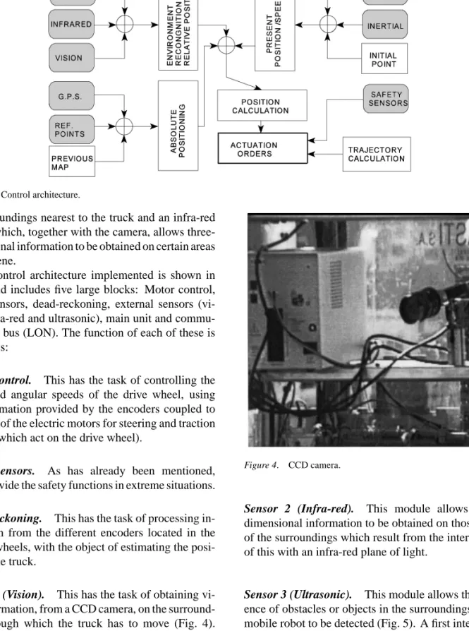
Figure 3. Control architecture.
the surroundings nearest to the truck and an infra-red system which, together with the camera, allows three-dimensional information to be obtained on certain areas in the scene.
The control architecture implemented is shown in Fig. 3 and includes five large blocks: Motor control, safety sensors, dead-reckoning, external sensors (vi-sion, infra-red and ultrasonic), main unit and commu-nications bus (LON). The function of each of these is as follows:
Motor Control. This has the task of controlling the linear and angular speeds of the drive wheel, using the information provided by the encoders coupled to the axles of the electric motors for steering and traction (both of which act on the drive wheel).
Safety Sensors. As has already been mentioned, these provide the safety functions in extreme situations. Dead-Reckoning. This has the task of processing in-formation from the different encoders located in the various wheels, with the object of estimating the posi-tion of the truck.
Sensor 1 (Vision). This has the task of obtaining vi-sual information, from a CCD camera, on the surround-ings through which the truck has to move (Fig. 4). It permits guiding along defined paths such as roads (whether painted lines exist or not). The functioning of this sensor system is the object of the second part of this article and is described more fully in Section 3 and following sections.
Figure 4. CCD camera.
Sensor 2 (Infra-red). This module allows three-dimensional information to be obtained on those parts of the surroundings which result from the intersection of this with an infra-red plane of light.
Sensor 3 (Ultrasonic). This module allows the pres-ence of obstacles or objects in the surroundings of the mobile robot to be detected (Fig. 5). A first interpreta-tion of the informainterpreta-tion obtained through these sensors permits obstacles to be detected and avoided. A more detailed analysis facilitates the identification of the ob-jects and the location of the vehicle with respect to same.
Figure 5. Ultrasonic sensors.
Main Unit. This module has the task of processing the high level information (the path to be followed, map of the surroundings, position of the obstacles, etc.) provided by the various sensors, in order to adapt them to the low level commands (steering and angular speed of the drive wheel) which the motor control system can adequately interpret, taking the physical model of the mobile robot and the type of control to be executed into account.
Communications Bus (LON). This has the task of communicating between the various aforementioned modules. Each block is provided with sufficient “telligence” for high level processing of the external in-formation received, so that the messages exchanged be-tween them are kept to a minimum. It is because of this that emphasis has been placed on reliability and speed (real time) in communications in the bus selected. A bus that provides these services and which also allows the reconfiguration of the system and allows flexibil-ity is the ECHELON (ECHELON, 1993). Each node in this bus has a link circuit called a “Neuronchip” which can be programmed in a high level language (NeuronC), thus facilitating the configuration of same (which variables are shared with other nodes) and the establishment of communications.
Kinematic Model of the Truck
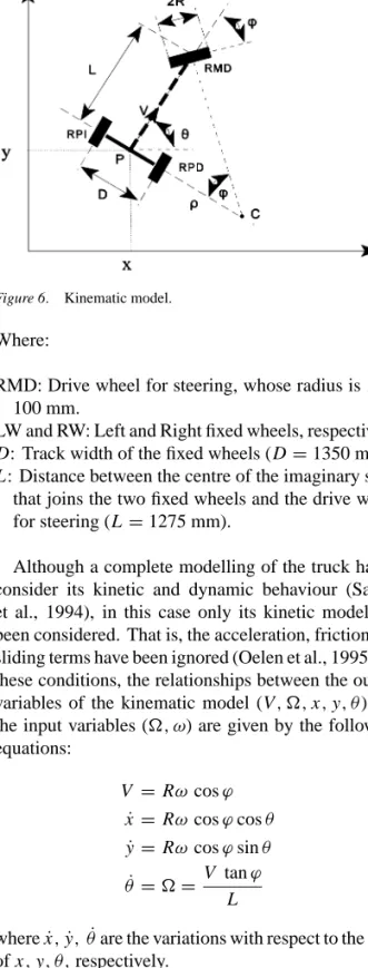
The industrial truck (ASTISA Fork Lift Truck GU-100-B) is a kinematic model such as the one shown in Fig. 6.
Figure 6. Kinematic model.
Where:
RMD: Drive wheel for steering, whose radius is R = 100 mm.
LW and RW: Left and Right fixed wheels, respectively.
D: Track width of the fixed wheels (D=1350 mm).
L: Distance between the centre of the imaginary shaft
that joins the two fixed wheels and the drive wheel for steering (L=1275 mm).
Although a complete modelling of the truck has to consider its kinetic and dynamic behaviour (Sarkar et al., 1994), in this case only its kinetic model has been considered. That is, the acceleration, friction and sliding terms have been ignored (Oelen et al., 1995). In these conditions, the relationships between the output variables of the kinematic model (V, Ä,x,y, θ) and the input variables (Ä, ω) are given by the following equations: V =Rωcosϕ ˙ x =Rωcosϕcosθ ˙ y=Rωcosϕsinθ ˙ θ =Ä= V tanϕ L (1)
wherex˙,y˙,θ˙are the variations with respect to the time of x,y, θ,respectively.
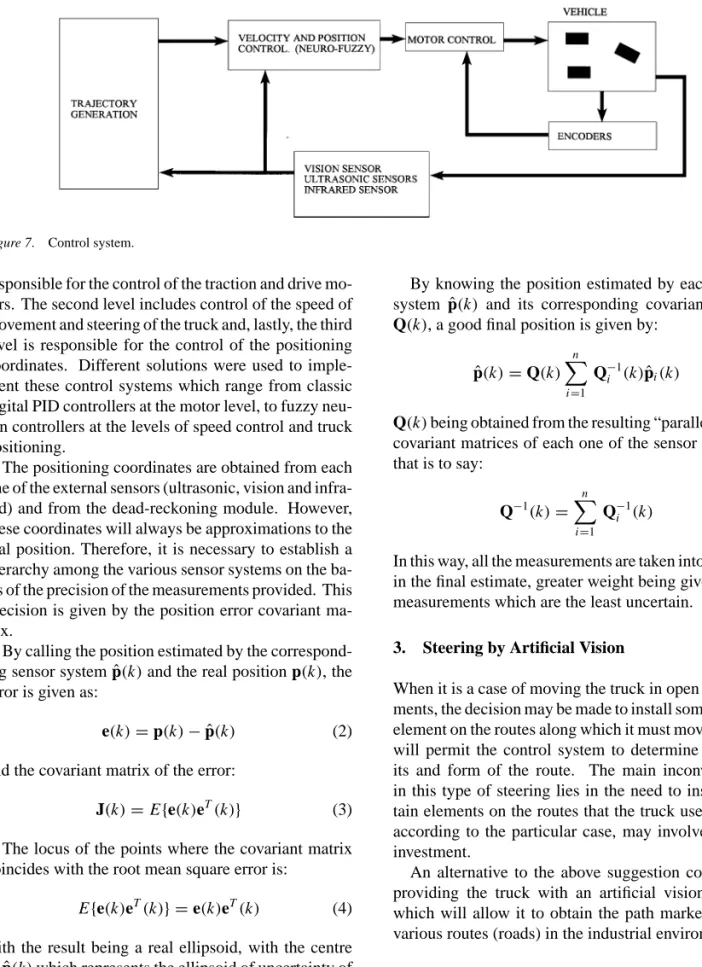
Control System
The control system can be seen in the block diagram in Fig. 7 and includes different levels. The lowest level is
Figure 7. Control system.
responsible for the control of the traction and drive mo-tors. The second level includes control of the speed of movement and steering of the truck and, lastly, the third level is responsible for the control of the positioning coordinates. Different solutions were used to imple-ment these control systems which range from classic digital PID controllers at the motor level, to fuzzy neu-ron controllers at the levels of speed control and truck positioning.
The positioning coordinates are obtained from each one of the external sensors (ultrasonic, vision and infra-red) and from the dead-reckoning module. However, these coordinates will always be approximations to the real position. Therefore, it is necessary to establish a hierarchy among the various sensor systems on the ba-sis of the precision of the measurements provided. This precision is given by the position error covariant ma-trix.
By calling the position estimated by the correspond-ing sensor systempˆ(k)and the real position p(k), the error is given as:
e(k)=p(k)− ˆp(k) (2) and the covariant matrix of the error:
J(k)=E{e(k)eT(k)} (3) The locus of the points where the covariant matrix coincides with the root mean square error is:
E{e(k)eT(k)} =e(k)eT(k) (4) with the result being a real ellipsoid, with the centre inpˆ(k)which represents the ellipsoid of uncertainty of the measurement estimated by the sensor. The greater the axes of the ellipsoid or the ellipse if working with its projection on the X -Y plane, the greater the uncertainty and the poorer the quality of the measurement made.
By knowing the position estimated by each sensor system pˆ(k) and its corresponding covariant matrix
Q(k), a good final position is given by:
ˆ p(k)=Q(k) n X i=1 Qi−1(k)ˆpi(k) (5)
Q(k)being obtained from the resulting “parallel” of the covariant matrices of each one of the sensor systems, that is to say: Q−1(k)= n X i=1 Q−i1(k) (6) In this way, all the measurements are taken into account in the final estimate, greater weight being given to the measurements which are the least uncertain.
3. Steering by Artificial Vision
When it is a case of moving the truck in open environ-ments, the decision may be made to install some type of element on the routes along which it must move, which will permit the control system to determine the lim-its and form of the route. The main inconvenience in this type of steering lies in the need to install cer-tain elements on the routes that the truck uses which, according to the particular case, may involve a large investment.
An alternative to the above suggestion consists of providing the truck with an artificial vision system which will allow it to obtain the path marked on the various routes (roads) in the industrial environment.
Outline of the Problem
An automated system for following roads has to con-sider the following problems (Pomerleau, 1993):
Figure 8. Schematic of vision system functioning.
— Changes in the state of the roads. — Changes in the lighting conditions. — Changes in the meteorological conditions. — The presence of obstacles (other moving objects). Constructing a system capable of dealing successfully with all these circumstances is no trivial matter when it also has to be considered that the processing time for an image has to be such to permit guiding at speeds which each application requires. In the case of the industrial truck, this restriction on the processing time is not excessive as the maximum speed at which it can move is 10 m/s.
General Description of the System for Following a Road for an Autonomous Industrial Vehicle (VIA)
The system for following a road tested in the VIA project attempts to approach the majority of the prob-lems described. A basic schematic of its functioning can be seen in Fig. 8.
The system has various algorithms for following a road: (a) detection of painted lines, (b) textural differ-ences between the road and non-road, (c) determination of the minimum width and (d) training of the neural networks. A model of the road with three parameters (a1, a2 and a3) was used in order to establish which
algorithm should be employed at any particular time. This was updated with the new measurements provided by the active system for following. When the mea-surements varied significantly from those predicted by the model, another algorithm for following was used and the model was adapted according to this new al-gorithm for following. As the following of the road was being carried out, a neural network was trained in such a way that, while there was no drastic change in the road conditions, or the paths were repeated, the neural network directly provided the information nec-essary for steering the vehicle. In this way, the system imitated the behaviour of a human driver who, as well as steering according to the markings that he finds on the road, memorizes situations, thus decreasing the re-sponse time when these are repeated.
Generating a Path
Generating a path begins with the schematic in Fig. 9, where P is the position of the centre point of the rear axle of the mobile robot at the present time; P0indicates where this point should be situated when the distance
l is covered, by following the road: d is the distance
from P to the edge of the road and d0is the distance that there must be between the edge and P0when l has been covered;θis the angle which must be zero in order to
Figure 9. Generating a path.
locate the mobile robot in a position parallel to the road and at the distance d0, after covering l metres. The dis-tance l is a parameter of the system for following fixed at 5 metres; d0is another parameter that represents the distance that there must be at all times between the mo-bile robot and the edge of the road (1 metre at present).
θis the measurement of the real position of the mobile robot with respect to the destination position, which can be calculated by knowing l,d and the equation for
the edge of the road, provided by the vision system. The control loop that allows the mobile robot to be positioned in position P0has the referenceθ=0.
Work Previous to Road Following
In general, the projects developed in other research centres apply artificial vision techniques for detecting certain characteristics present in the video images taken of the road in front of the vehicle in order to determine the path that the vehicle has to follow from its relative position on the image. Almost all these systems are centred on detecting some specific characteristic, such as painted lines on the road (Dickmanns et al., 1994). Others, detect the regions on the image that represent the road basing this on characteristics such as colour (Turk et al., 1988) or texture (Thorpe, 1990). An al-ternative approach consists of combining vision with learning techniques (basically neural networks) in such a way that the learning process is the neural network itself that establishes the characteristics that define the path along the road (Pomerleau, 1993).
One of the most important tasks in autonomous guiding along a road was executed by the group of Prof. E.D. Dickmanns at the Bundeswehr University in Munich. In his latest work (Dickmanns et al., 1994), within the Prometheus III project in the EUREKA pro-gramme of the European Community, a Mercedes 500 SEI car (VaMoRs-P) was equipped with a complex sen-sor system (4 colour cameras, three inertial sensen-sors, a tachometer and angle sensors) and a sophisticated pro-cessing system (60 transputers and various PC 486’s) with the object of driving the vehicle along motorways at speeds of up to 130 km/h.
In the United States, one of the most outstanding projects was the NavLab project of Carnegie Mellow University. Various algorithms were tried out in this project for the detection of the edges of the road (Pomerleau, 1993), which was started in 1986. The one that has given the best results to date is based on the training of a neural network whose input is a low resolution 30×30 image and whose output Xa is the direct position that the wheels of the vehicle have to have in order to follow the road. This system, called ALVINN, managed to drive the test vehicle, NAVLAB 1, for 21.2 miles at speed of up to 55 miles/h. The neural network functions reasonably well when it is trained in conditions and on roads similar to those along which the vehicle is travelling. When changes in the road conditions are produced on the paths followed by the mobile robot, it is necessary to switch to another trained neural network until these new conditions have passed. In order to solve the problem of how and to which neural network to switch, a super-connecting structure—MANIAC—has been proposed which in-corporates multiple single networks of the ALVINN type, each one pre-trained for a particular type of road.
In the PATH programme (Partners for Advanced and Transit Highways) in the American State of California, with the participation of the Institute of Transportation Studies of the University of California in Berkeley, ex-tensive work has been carried out since 1986 on the autonomous steering of vehicles along roads. At the present time, experiments are being carried out with magnetic sensors located on the road, to facilitate lat-eral control of the vehicle, and with a Doppler radar for detecting obstacles and the longitudinal control of the vehicle. Research is being done on the possibility of integrating these sensors with visual information. The vision module is based on stereovision to obtain the position of the lines on the road (Koller I., 1995).
4. Algorithms Used for VIA Area of Interest
An area of interest was established in the image which contains sufficient information to allow the steering of the mobile robot with the object of reducing the pro-cessing time to a minimum. The area under study, on the other hand, was modified according to the charac-teristics of the road in question and the steering speed. In this way, the steering speed on straight stretches can increase significantly and it is therefore necessary to be able to detect any possible bends sufficiently in ad-vance, by locating the area under study in the upper area of the image. On stretches with bends, the speed of the vehicle decreases so the study window is centred near the mobile robot with the object of following the bend perfectly.
Algorithm for Following Painted Lines
Using three bands of colour (r,g,b) per image,
pro-vided by the image acquisition system, an image with an intensity, I , is obtained, as follows:
I = r
1 3(r
2+g2+b2) (7)
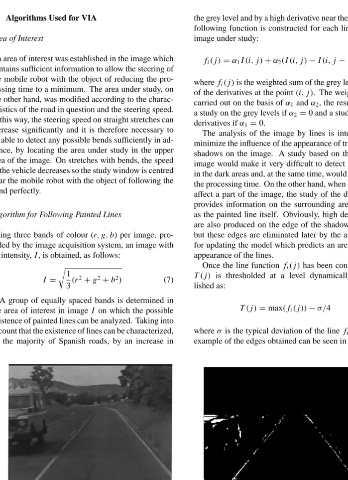
A group of equally spaced bands is determined in the area of interest in image I on which the possible existence of painted lines can be analyzed. Taking into account that the existence of lines can be characterized, on the majority of Spanish roads, by an increase in
Figure 10. Gray level image (a). Lines detected (b).
the grey level and by a high derivative near the line, the following function is constructed for each line of the image under study:
fi(j)=α1I(i,j)+α2(I(i,j)−I(i,j−1)) (8) where fi(j)is the weighted sum of the grey levels and of the derivatives at the point(i,j). The weighting is carried out on the basis ofα1andα2, the result being a study on the grey levels ifα2 =0 and a study on the derivatives ifα1=0.
The analysis of the image by lines is intended to minimize the influence of the appearance of transverse shadows on the image. A study based on the whole image would make it very difficult to detect the lines in the dark areas and, at the same time, would increase the processing time. On the other hand, when shadows affect a part of the image, the study of the derivative provides information on the surrounding areas, such as the painted line itself. Obviously, high derivatives are also produced on the edge of the shadowed area, but these edges are eliminated later by the algorithm for updating the model which predicts an area for the appearance of the lines.
Once the line function fi(j)has been constructed,
T(j) is thresholded at a level dynamically estab-lished as:
T(j)=max(fi(j))−σ/4 (9) whereσ is the typical deviation of the line fi(j). An example of the edges obtained can be seen in Fig. 10.
Figure 11. Image with shadows (a). Enhanced road image (b).
Algorithm for Following the Road According to its Width
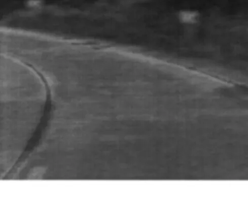
When a mobile robot is driven along a road it is only necessary to have sufficient roadwidth, with the restric-tions of steering along the right hand lane, at a certain distance from the edge and without colliding with the vehicles obstructing the path. For this, another algo-rithm available in VIA, in the case of it not being pos-sible to detect painted lines, consists of searching for sufficient roadwidth for the mobile robot to be able to move.
An image in grey levels is constructed from three colour bands (r,g,b), in which the road is
empha-sised and shadow is eliminated as far as possible. In (Pomerleau, 1993 and Crisman, 1988) it is shown that by adding standard brilliance to the blue band, a cer-tain type of shadow can be eliminated. What is more, the difference between bands r and g, emphasises the road. In our algorithm, a grey image is constructed, both things being achieved simultaneously. To do this
I is constructed, as follows: I =b+ b−r
r+g+b (10)
Figure 11 shows the elimination of shadows and the relief of the road.
Once image I has been obtained, it is standardized and thresholded starting from the fact that the road has been highlighted and evened out, and that, in these conditions, a simple thresholding allows the road to be detected. The choice of the threshold level is made dynamically. The thresholding process is started at a certain level, ul, the resulting width of the road is
determined line by line and a check is made to ensure that it is sufficient for the robot to pass. If it is not, the threshold level is decreased until the necessary width is achieved. The points which define the greatest width that can be achieved on each line are then detected and a check is made to ensure that they are compatible with the aforementioned ones for the road model. In the case of the points on the model not being compatible, they are rejected and an attempt is made to search the road using another algorithm. The threshold level for the following search is initially located as a function of the value achieved in the previous iteration.
This algorithm functions very well for detecting the right hand side of the road which, in fact, is more impor-tant when driving the mobile robot. Figure 12 shows the result of applying the algorithm to the image in Fig. 11.
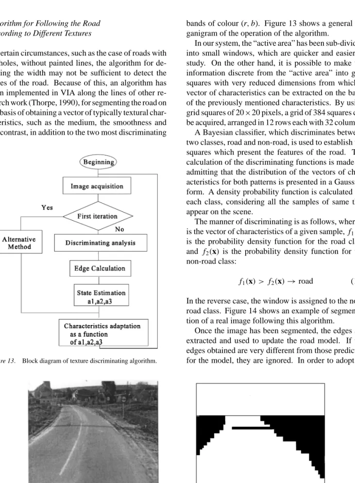
Algorithm for Following the Road According to Different Textures
In certain circumstances, such as the case of roads with potholes, without painted lines, the algorithm for de-tecting the width may not be sufficient to detect the edges of the road. Because of this, an algorithm has been implemented in VIA along the lines of other re-search work (Thorpe, 1990), for segmenting the road on the basis of obtaining a vector of typically textural char-acteristics, such as the medium, the smoothness and the contrast, in addition to the two most discriminating
Figure 13. Block diagram of texture discriminating algorithm.
Figure 14. Original image and segmentation obtained.
bands of colour (r,b). Figure 13 shows a general
or-ganigram of the operation of the algorithm.
In our system, the “active area” has been sub-divided into small windows, which are quicker and easier to study. On the other hand, it is possible to make the information discrete from the “active area” into grid squares with very reduced dimensions from which a vector of characteristics can be extracted on the basis of the previously mentioned characteristics. By using grid squares of 20×20 pixels, a grid of 384 squares can be acquired, arranged in 12 rows each with 32 columns. A Bayesian classifier, which discriminates between two classes, road and non-road, is used to establish the squares which present the features of the road. The calculation of the discriminating functions is made by admitting that the distribution of the vectors of char-acteristics for both patterns is presented in a Gaussian form. A density probability function is calculated for each class, considering all the samples of same that appear on the scene.
The manner of discriminating is as follows, where x is the vector of characteristics of a given sample, f1(x) is the probability density function for the road class and f2(x)is the probability density function for the non-road class:
f1(x) > f2(x)→road (11) In the reverse case, the window is assigned to the non-road class. Figure 14 shows an example of segmenta-tion of a real image following this algorithm.
Once the image has been segmented, the edges are extracted and used to update the road model. If the edges obtained are very different from those predicted for the model, they are ignored. In order to adopt an
algorithm, it is necessary to work with a model for each edge of the road, in order to determine the squares that belong to each class in the active area. Finally, the discriminating functions are updated in such a way that, in the following classification, any possible changes in the texture of the road will have been taken into account.
Neural Network.
The neural network is trained at the same time as the system for following the road is providing the points necessary for defining the road model (see Section 5), by inputting the reduced image to the windows and the value of the parameter that defines the path to be followed (θ) as the output. When the network has been sufficiently trained, its output allows steering by the system with a response time clearly less than that in the algorithms already described.
The architecture of the neural network is similar to that employed by Pomerleau (1993) but, with the methodology for training being substantially modified. In (Pomerleau, 1993) the training is carried out while a driver steers the mobile robot along the road which is the object of the test. This method has the disadvantage of the need for previous learning of the autonomous steering and dependence on the kinetic model of the mobile robot, as the drive commands depend on this.
The output provided by the neural network once functioning allows a confidence level to be established in such a way that when this is insufficient, another algorithm for following the road is activated and the network weightings are stored, in case the previous steering conditions should be produced again. At the present time, our system is capable of storing up to 20 different networks following the FIFO principle.
While following the road, without the action of any network and at the same time as a new network is being trained, one of the networks already stored is selected every 5 frames and a check is made on whether its re-sponse is compatible with that predicted by the model. If it is, the network is activated and has the task of steer-ing the mobile robot. In this way, if the mobile robot moves through an area which has already been crossed previously, the system will need 100 frames to recover the network that was trained in this section, in the worst of cases. 100 frames implies an average steering speed of 5 m/s with a processing time per frame of 100 ms and that the robot will cover 50 m as a maximum until the system is capable of remembering the road.
5. Model of the Road
The correct functioning of the algorithms described above requires the existence of a prediction of the path marked on the road, with the object of determining whether the results obtained by the algorithm are co-herent. At the same time, two types of uncertainties are resolved. The first is the uncertainty over the speed with which the road changes direction as a function of time (supposing a constant speed). The second is the uncertainty over whether the characteristics sought will be found in the following image and, in the case of finding them, what state they will be in and what quality they will have.
Model for Representing the Edges of the Road
When it comes to choosing the model to represent the road, two important alternatives are introduced, working directly on the flat image in two dimensions or previously transforming the flat image to three-dimensional coordinates. The first option has the ad-vantage of simplifying the calculations and therefore facilitates real time control of the mobile robot. How-ever, the model may be less exact than the one that operates in three-dimensional space. The second op-tion has the advantage of being able to operate with a model, the clotoidal model, which is comparable to the one employed for the projection and routing of roads. However, it is more costly from the point of view of calculating and more sensitive to maladjustments of the camera.
In our case, a model which operates on the image in two dimensions was chosen to optimize the process-ing time, the efficiency of which was compared with other work (Schneiderman and Nashman, 1994). The edges of the road (or the lines that define the lane for the truck to pass) are modelled by means of a sec-ond degree polynomial, one for each edge, on the flat image.
j=a1·i2+a2·i+a3 (12)
where j is the column and i is the row, a1,a2 and a3 determine the form and position of the model of the edge. The final points for each model are determined by the intersection of the equation that represents the model and the limits of the window of interest.
Updating the Model
The points on the edge of the road obtained by the al-gorithm for active following of the road are used to update the model of the edge. At the time of updating the model, an attempt must be made to make the result sufficiently robust. In order to do this, a compromise must be made between the robustness of the model (considering a long series of images when calculating this) and the response capacity faced with changes in the road (using a short sequence of images). Further-more, as the number of coherent points on the edge that can be calculated from one image to another can vary, depending on the appearance of shadows, pot-holes, changes in light, etc., an image with a lot of points on the edge in the model of the road must have more influence than another image that only has few points.
Procedure for Updating the Model
The following cost function is minimized for updating the model: JR= t X p=0 à λt−p Np X a=1 £ jp,a− ¡ a3+a2ip,a+a1i2p,a ¢¤2 ! (13) where t corresponds to the current image, Np, in the number of points achieved in the image p. Each term in the cost function represents the points on the edge obtained at any given moment. The influence of each term in the final expression will be given by the number of points on the edge obtained for that image, so that images with a lot of points will have more influence on the result that those with fewer points. On the other hand, images previous to the current one are taken into account in the cost function in order to achieve a robust estimate. However, to avoid the algorithm being insen-sitive to changes in the path on the road, the points in the previous images cannot be weighted in the same manner as the current ones. An exponentially decreas-ing weightdecreas-ing is therefore established, by multiplydecreas-ing each term by a power ofλ, so that the oldest images have the least influence on the final model.
The parameterλ, variable between 0 and 1 allows the influence of past images to be increased or de-creased. The greater the value ofλ, the greater will
be the influence of the past sequence, eventually arriv-ing at the case where, withλ=1, all the images have an equal influence on the training of the model, result-ing in a system that is highly insensitive to changes in the path marked on the road. Small values ofλ mini-mize the influence of the previous images, decreasing the robustness of the model and making it more sensi-tive to changes in the path. In the extreme case ofλ=0, only the current image will be taken into account in the training of the model.
An adjustment ofλis essential in order to achieve a robust system which is sensitive to changes in the path on the road at the same time. In order to avoid the problem of a saturation of the algorithm on straight stretches, the value ofλis dynamically modified while the road is being followed. On stretches where there are no significant changes in the path, the case may occur where the algorithm becomes insensitive to any possible later changes (e.g., a bend after a long straight stretch), because of this the value ofλis governed by the following expression:
λ=a1∗α+λmin (14) On straight stretches a1is practically 0, for which rea-son the algorithm is prepared to detect bends. On stretches with bends,λincreases so that the importance of past paths also increases.
Recursive Updating of the Model
The minimizing of the cost function employed requires a great number of calculations which have a negative effect on the system processing time and, therefore, on the final qualities of same. Because of this the updat-ing of the model is expressed again recursively, estab-lishing a1,a2 and a3 as the current state of the sys-tem. When new points on the edge are obtained, the new state is calculated by using these new points to-gether with the previous state and the covariant matrix of states, which represent the entire previous history. To sum up, this updating consists of three consecutive calculations:
(a) The points on the edge estimated by the model are calculated:
ˆ
(b) The estimated covariant of states is updated: P(n)= 1 λ[P(n−1)−K(n)H(n)P(n−1)] where K(n)=P(n−1)H0(n)(λI+H(n) ×P(n−1)H0(n))−1 (16) (c) The estimated state is updated:
x(n)=x(n−1)+K(n)[z(n)− ˆz(n)] (17) where z(n)= jn,1 jn,2 . . . jn,Nn H(n)= 1 in,1 i2n,1 1 in,2 i2n,2 . . . . 1 in,Nn in2,Nn x(n−1)= a3 a2 a1
x(n−1)represents the estimated state at the moment
n−1.P(n−1)represents an estimate of the states co-variant. This algorithm is known as recursive square minimums with decreasing exponential weighting (MCRP).
Determination of the Active Algorithm and Switching Between Algorithms
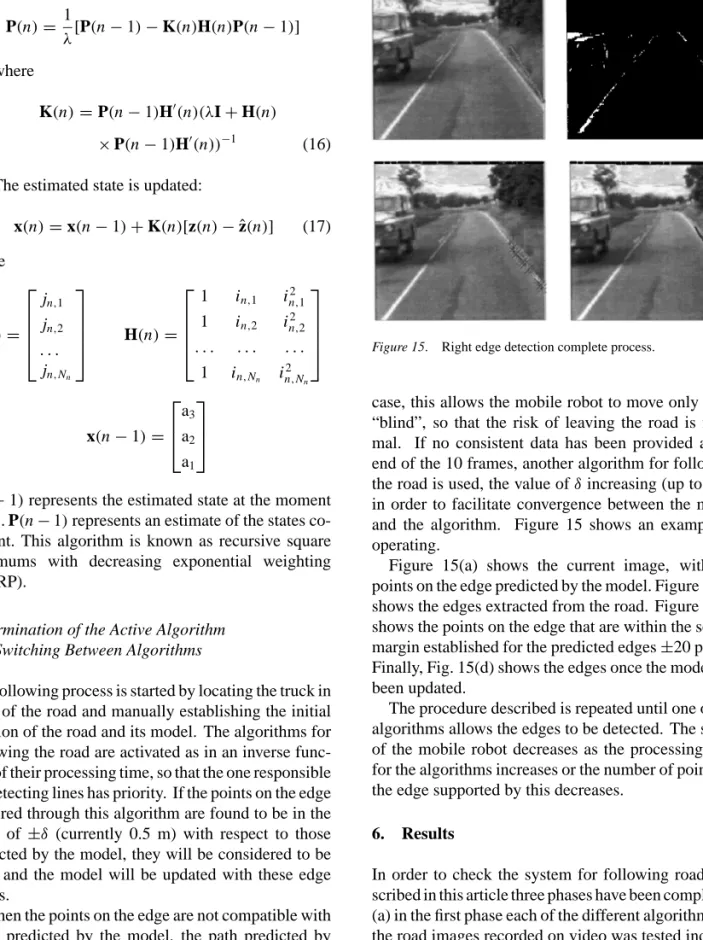
The following process is started by locating the truck in front of the road and manually establishing the initial position of the road and its model. The algorithms for following the road are activated as in an inverse func-tion of their processing time, so that the one responsible for detecting lines has priority. If the points on the edge acquired through this algorithm are found to be in the order of ±δ (currently 0.5 m) with respect to those predicted by the model, they will be considered to be valid and the model will be updated with these edge points.
When the points on the edge are not compatible with those predicted by the model, the path predicted by the model will be maintained for 10 frames, in the hope of recovering consistent data. The choice of 10 frames has been made for safety reasons as, in the worst
Figure 15. Right edge detection complete process.
case, this allows the mobile robot to move only 10 m “blind”, so that the risk of leaving the road is mini-mal. If no consistent data has been provided at the end of the 10 frames, another algorithm for following the road is used, the value ofδincreasing (up to 1 m) in order to facilitate convergence between the model and the algorithm. Figure 15 shows an example of operating.
Figure 15(a) shows the current image, with the points on the edge predicted by the model. Figure 15(b) shows the edges extracted from the road. Figure 15(c) shows the points on the edge that are within the search margin established for the predicted edges±20 pixels. Finally, Fig. 15(d) shows the edges once the model has been updated.
The procedure described is repeated until one of the algorithms allows the edges to be detected. The speed of the mobile robot decreases as the processing time for the algorithms increases or the number of points on the edge supported by this decreases.
6. Results
In order to check the system for following roads de-scribed in this article three phases have been completed: (a) in the first phase each of the different algorithms for the road images recorded on video was tested individ-ually under various light, climatic and seasonal condi-tions; (b) this was followed by testing the system for integrating algorithms described for the same images
and (c) finally, tests were made in open environments using the industrial truck described, over a stretch of two kilometres on the University of Alcal´a campus.
6.1. Individual Tests of Each Algorithm
Each algorithm was individually tested on images cor-responding to a previously recorded section of approx-imately 15 kilometres on various roads under different circumstances. The measurements taken for establish-ing the effectiveness of the algorithms were: (a) the number of points on the edge obtained within the an-ticipated margin, according to the estimated position on the road, (b) the average rms error between the points obtained on the edge and those estimated by the road model, (c) the index of confidence calculated as the ratio between the number of points obtained and the average error and, finally, (d) the standardized error of states, measured as:
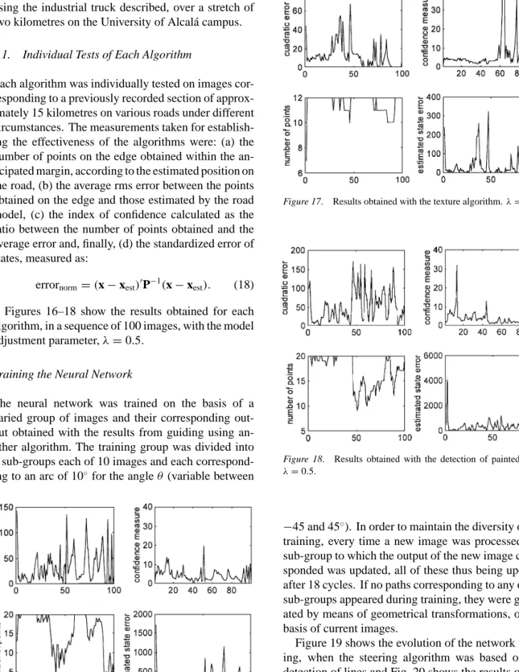
errornorm=(x−xest)0P−1(x−xest). (18) Figures 16–18 show the results obtained for each algorithm, in a sequence of 100 images, with the model adjustment parameter,λ=0.5.
Training the Neural Network
The neural network was trained on the basis of a varied group of images and their corresponding out-put obtained with the results from guiding using an-other algorithm. The training group was divided into 9 sub-groups each of 10 images and each correspond-ing to an arc of 10◦for the angleθ (variable between
Figure 16. Results obtained with the width search algorithm.λ= 0.5.
Figure 17. Results obtained with the texture algorithm.λ=0.5.
Figure 18. Results obtained with the detection of painted lines.
λ=0.5.
−45 and 45◦). In order to maintain the diversity of the training, every time a new image was processed, the sub-group to which the output of the new image corre-sponded was updated, all of these thus being updated after 18 cycles. If no paths corresponding to any of the sub-groups appeared during training, they were gener-ated by means of geometrical transformations, on the basis of current images.
Figure 19 shows the evolution of the network train-ing, when the steering algorithm was based on the detection of lines and Fig. 20 shows the results of fol-lowing the road, measured in terms of average rms error, once the network had been trained and the guid-ing of the mobile robot assumed. On average, network training required 100 cycles.
Table 1. Results obtained for various test.
Light conditions Average speed Average deviation Typical deviation Other comments Sunny, middle hours 5.45 m/s 10.87 cm 3.19 cm
Sunny, sun at sunset 3.32 m/s 17.34 cm 5.47 cm Stopped at 100 m of finish
Cloudy 5.35 m/s 11.03 cm 3.25 cm
Sunny, middle hours 5 m/s 7.16 cm 2.52 cm Constant speed
Figure 19. Evolution of the network training.
Figure 20. Results of following with de neural network. Tests on the Industrial Truck
in Open Environments
The run designed for checking the efficiency of the guiding algorithms was on the University of Alcalá campus and was approximately two kilometres in length, with two alternate sections of 500 metres with
painted lines and another two without any type of sig-nalling, so that the system of steering by artificial vision had to switch between the various algorithms in order to complete the run. The autonomously guided truck completed the above run in 6 minutes at an average speed of 5 m/s under normal ambient conditions (mid-dle hours of the day and sunny). Figure 21 shows the truck during the run and the PC used to execute the algorithms described.
Although there is no existing standard for establish-ing the qualities of an automatic system for followestablish-ing roads, the average deviation with respect to the ideal path was measured (driving at 1 metre from the edge) and the results obtained for various tests under different circumstances are shown in Table 1.
The run made at a constant speed of 5 m/s gives an average deviation of less than that obtained when the speed is variable due to the fact that, in the latter case, the speed was calculated using a fuzzy controller in which small oscillations in its tuning could not be avoided. Finally, when the light conditions were ad-verse, the algorithms did not function as well, the av-erage steering speed being decreased. In the extreme case of the sun at sunset being in front of the truck, following could not be completed as the colour camera became saturated.
To conclude, compared with other systems, the one presented here permits guiding on almost all types of roads, with adaptations to changes in the markings on the road, width and climatic conditions. In compari-son with learning algorithms such as the one used in (Pomerleau, 1993), this system has similar advantages, without the need for previous training as the network learns at the same time as the system is being steered by another type of algorithm. When comparing it with the work in (Dickmanns et al., 1994), this system is more modest, but is capable of guiding along roads without painted lines and the cost of the hardware for the sys-tem is considerably less, which makes it more likely to be used in the industrial world which, when all is said and done, is the final objective of this work.
Figure 21. Truck during the run and the PC used to execute the algorithms.
Acknowledgments
The work presented has been possible thanks to a re-search project financed by the CICYT (VIA project, TAP94-0656-C03-01).
References
Crisman, J.D. and Thorpe, C.E. 1988. Color vision for road follow-ing. In Proc. of Mobile Robots III.
Dickmanns, E.D., Behringer, R., Dickmanns, D., Hildebrant, T., Mauer, M., Thomanek, F., and Shielhlen, J. 1994. The seeing passenger car ‘VaMoRs-P’. In Proc. of Int. Symp. on Intelligent
Vehicles, Paris.
ECHELON. 1993. LonWorks Technology: Intelligent Distributed
Control.
Koller, D., Luong, T., and Jitendra, M. 1995. An integrated stereo-based approach to automatic vehicle guidance. In Proc. Int.
Con-ference on Computer Vision, Boston.
Mazo, M. and Maravall, D. 1990. Guidance of an autonomous vehicle by visual feedback. Cybernetics and Systems, 21:257–266. Mazo, M., Rodríguez, F.J., L´azaro, J.L., Ure˜na, J., García, J.J., and
Santiso, S. 1995. Electronic control of a wheelchair guided by voice commands. Control Eng. Practice, 3(5):665–674. Oelen, W., Berghuis, H., Nijmeijer, H., Canudas de Wit, C. 1995.
Hybrid stabilizing control on a real mobile robot. IEEE Robotics
& Automation Magazine, 2(2):16–23.
Pomerleau, D. 1993. Neural Network Perception for Mobile Robot
Guidance, Kluwer: Boston.
Sarkar, N., Yun, X., and Kumar, V. 1994. Control of mechanical systems with rolling constraints: Application to dynamic mobile robots. Int. Journal of Robotics Research, 13(1).
Schneiderman, H. and Nashman, M. 1994. A discriminating fea-ture tracker for vision based autonomous driving. IEEE Trans. on
Robotics and Automation, 10(6):769–775.
Thorpe, C. 1990. Vision and Navigation: The Carnigie Mellon
Navlab, Kluwer: Boston.
Turk, A.M., Morgenthaler, D., Gremban, D., and Marra, M. 1988. VITS—A vision system for autonomous land vehicle navigation.
IEEE Trans. on Pattern Analysis and Machine Intelligence,
10(3):342–361.
Fco Javier Rodríguez received a Ph.D. in Electronics Engineering
from University of Alcal´a in 1997, a Telecommunication Engineer-ing degree from Polytechnic University of Madrid, in 1990, and a Technical Telecommunications Engineering degree, in 1985, also from Polytechnic University of Madrid. He has worked at private electronic industry for two years, and, from 1986, is a Professor in the Department of Electronic at the University of Alcalá de Henares. His current work covers the areas of Robotics, Artificial Vision, Neural Nets, Fuzzy Logic Controllers and Real Time Processing.
Manuel Mazo received a Electronics Engineering,
degrees from Polytechnic University of Madrid (Spain) in 1976, 1982 and 1988, respectively. He is a Professor at the Technical School of Alcalá from 1976. He has conducted several research works in Arti-ficial Vision and Multisensor Integration applied to Mobile Robots. His areas of interest are Mobile Robots, Artificial Vision and Speech Recognition. He is also a member of IEEE.
Miguel Angel Sotelo received a Technical Telecommunications
En-gineering degree from Alcalá de Henares University, Spain, in 1992 and Telecommunication Engineering degree from Polytechnic Uni-versity of Madrid, Spain, in 1996. He is presently working in a research project about the guidance of Mobile Robots by Artificial Vision.