Article in Nuclear Fusion · July 2019 DOI: 10.1088/1741-4326/ab2ea9 CITATIONS 3 READS 229 7 authors, including:
Some of the authors of this publication are also working on these related projects:
Smart RHC-IoTView project
Development of a multi-machine inter-shot disruption analysis toolView project Alessandro Pau
École Polytechnique Fédérale de Lausanne 52PUBLICATIONS 368CITATIONS
SEE PROFILE
A. Fanni
Università degli studi di Cagliari 183PUBLICATIONS 1,704CITATIONS
SEE PROFILE S. Carcangiu
Università degli studi di Cagliari 59PUBLICATIONS 152CITATIONS
SEE PROFILE
Barbara Cannas
Università degli studi di Cagliari 143PUBLICATIONS 1,497CITATIONS
SEE PROFILE
All content following this page was uploaded by Alessandro Pau on 04 July 2019.
To cite this article before publication: Alessandro Pau et al 2019 Nucl. Fusion in press https://doi.org/10.1088/1741-4326/ab2ea9
Manuscript version: Accepted Manuscript
Accepted Manuscript is “the version of the article accepted for publication including all changes made as a result of the peer review process, and which may also include the addition to the article by IOP Publishing of a header, an article ID, a cover sheet and/or an ‘Accepted Manuscript’ watermark, but excluding any other editing, typesetting or other changes made by IOP Publishing and/or its licensors” This Accepted Manuscript is © EURATOM 2019.
During the embargo period (the 12 month period from the publication of the Version of Record of this article), the Accepted Manuscript is fully protected by copyright and cannot be reused or reposted elsewhere.
As the Version of Record of this article is going to be / has been published on a subscription basis, this Accepted Manuscript is available for reuse under a CC BY-NC-ND 3.0 licence after the 12 month embargo period.
After the embargo period, everyone is permitted to use copy and redistribute this article for non-commercial purposes only, provided that they adhere to all the terms of the licence https://creativecommons.org/licences/by-nc-nd/3.0
Although reasonable endeavours have been taken to obtain all necessary permissions from third parties to include their copyrighted content within this article, their full citation and copyright line may not be present in this Accepted Manuscript version. Before using any content from this article, please refer to the Version of Record on IOPscience once published for full citation and copyright details, as permissions will likely be required. All third party content is fully copyright protected, unless specifically stated otherwise in the figure caption in the Version of Record. View the article online for updates and enhancements.
A Machine Learning approach based on Generative Topographic
Mapping for disruption prevention and avoidance at JET
A. Pau1, 2, A. Fanni2, S. Carcangiu2, B. Cannas2, G. Sias2, A. Murari3, F. Rimini4 and the JET Contributors*
1Ecole Polytechnique Fédérale de Lausanne (EPFL), Swiss Plasma Center (SPC), CH-1015 Lausanne, Switzerland
2Electrical and Electronic Engineering Dept.-University of Cagliari, Piazza D’Armi, 09123, Cagliari, Italy.
3 Consorzio RFX-Associazione - EURATOM ENEA per la Fusione, Padova, Italy
4 CCFE, Culham Science Centre, OX14 3DB Abingdon, UK.
* See the author list of “X. Litaudon et al 2017, Nucl. Fusion 57 102001.
Abstract-Predictive capabilities better than 95%, and very limited false alarms, are demanding requirements for reliable disruption prediction systems in tokamaks such as JET or, in the near future, ITER. The prediction of an upcoming disruption has to be provided sufficiently in advance in order to apply effective disruption avoidance or mitigation actions preventing the machine to be damaged.
In this paper, following the typical machine learning workflow, a Generative Topographic Mapping (GTM) of the operational space of JET has been built using a set of disrupted and regularly terminated discharges. In order to build the predictive model, a suitable set of dimensionless, machine-independent, physics-based features have been synthesized, which make use of 1D plasma profiles information, rather than simple zero-D time series. The use of such predicting features, together with the power of the GTM in fitting the model to the data, allows obtaining, in an unsupervised way, a 2-dimensional map of the multi-dimensional parameter space of JET, where it is possible to identify a boundary separating the region free from disruption from the disruption region. In addition to helping in operational boundaries studies, the GTM map can also be used for disruption prediction exploiting the potentiality of the developed GTM toolbox to monitor the discharge dynamics. Following the trajectory of a discharge on the map throughout the different regions, an alarm is triggered depending on the disruption risk of these regions. The proposed approach to predict disruptions has been evaluated on a training and an independent test set, allowing to achieve very good performance with only one tardive detection and a limited number of false detections. The warning times are suitable for avoidance purposes and, more important, the detections are consistent with physics causes and mechanisms that destabilize the plasma leading to disruptions.
I.
Introduction
Avoiding plasma disruptions will be one of the major concerns for the next generation of tokamaks such as ITER and DEMO. Disruptions, indeed, can cause severe damage to the structural integrity of the machines, forcing unexpected and eventually long maintenance interventions, which significantly reduce the availability of the device [1]. Avoiding disruptions or mitigating their effects requires quite different actions. For avoidance, the chain of events preceding the disruption has to be detected [2] [3] and suitable interventions have to be performed either to fully recover the nominal plasma parameters, keeping the plasma within the pre-programmed operation window, or at most to terminate it in a controlled way. To this purpose, sufficiently long warning times have to be provided to the disruption avoidance system. For mitigation, massive amount of gas or pellets can be injected into the plasma to increase the radiation, with the aim of reducing thermal and electromagnetic loads.
The plasma control system (PCS) on ITER, as well as the one on JET, will necessitate the availability of reliable triggers that have to satisfy different requirements, depending on whether they are intended for avoidance or mitigation purposes. The reliability and the effectiveness of such triggers can be defined in terms of warning time (that is the time between the trigger and the time of disruption), correct predictions, missed and false alarms. In the case of the disruption mitigation system (DMS), the requirements for the warning time are less stringent [4], and a mandatory limit is set by the system latency time. For the disruption mitigation
3 4 5 6 7 8 9 10 11 12 13 14 15 16 17 18 19 20 21 22 23 24 25 26 27 28 29 30 31 32 33 34 35 36 37 38 39 40 41 42 43 44 45 46 47 48 49 50 51 52 53 54 55 56 57 58 59 60
Accepted Manuscript
valves (DMV) on JET, a working assumption for the minimum warning time is 10 ms, whereas, according to the present design, for the shattered pellet injectors (SPI) of the ITER DMS it will be 30 ms. In the case of disruption avoidance, the minimum warning time depends on the combination of several factors, such as the type of disruption, the time scales involved by physics mechanisms playing a role, and the time required by the control actuators to intervene on the plasma state. As far as the success rate figures of merit are concerned, correct predictions and false alarm rates, again, are defined depending on the requirements of the specific machine. For ITER DMS, the requirements vary depending, on the one hand, on the machine operational phase and on plasma parameters and, on the other hand, on the disruption phenomena to be detected. During the operations at full performance, the failure rate in the detection of the current quench (CQ) and the vertical displacement event (VDE), which is needed to protect the machine against electromagnetic forces and the release of magnetic energy, should be less than 1%. The failure rate in the detection of the thermal quench (TQ), needed for the mitigation of the associated thermal loads, should be lower than 5%.
The disruption detection system in JET is presently based on the thresholds of single signals or a combination of them, such as the locked mode signal amplitude, the total plasma energy, the plasma current, the loop voltage signals, or the peaking of the radiated power. Nevertheless, these MHD indicators or plasma control parameters may not always be the best early predictors for the disruption onset, because of their late appearance in the chain of events leading to disruption. Hence the need to monitor other quantities, often closely linked to the physics mechanisms that destabilize the discharge, such as the main kinetic plasma profiles, the radiation distribution, and the internal inductance [5].
The new design of the Plasma Event and TRigger for Avoidance (PETRA), being implemented in JET, foresees a cascade of a real time event detector block and the triggers handling to the already existent Real Time Protection System (RTPS) and Real Time Central Control (RTCC) units. The event detection system will comprise several disruption detection systems based on both physics-based disruption predictors and data driven predictors.
Up to now, disruption prediction systems for mitigation have been widely proposed on existing tokamaks. Physics basis for disruption prediction and detection have been discussed in [6],[7]. Several contributions have been proposed in the literature, aimed to develop disruption predictions using supervised data-based methods in JET [8], [9], ASDEX Upgrade [10], [11], J-TEXT [12], and DIII-D [13], only to quote some of them. In these papers, several plasma parameters, from a set of regularly terminated discharges, were used to describe the plasma operational space free from disruptions. Moreover, in order to describe the disrupted operational
space, a set of disrupted discharges was used and an unstable pre-disrupted phase was statistically or
heuristically identified and assumed equal for all the disruptions in the data base. This last choice introduced inconsistency in the prediction model that justify the prediction errors, even if they are generally limited to few tens of percent. These data-based models were unavoidably affected by the a priori selection of the training examples for the different classes they were supposed to predict. Indeed, the characterization of the boundary separating the different disruption classes might vary significantly, depending on the selection of the training examples; therefore, a proper selection of a pre-disruptive phase plays a key role on the performance of the
model. In the present paper, for each disruptive discharge, a proper unstable pre-disrupted phase has been
identified, which corresponds to the start of the chain of events leading to the disruption.
In addition, more general aspects concerning the generalization and the capability to extrapolate to new operational domains (new scenarios and/or new machines) have prevented machine learning methods from being considered as a viable and reliable solution for prediction and avoidance of disruptions. Firstly, as previously mentioned, they require an initial database to build and train the model. Secondly, all these data base models are strictly dependent on the choice of the parameters used to describe the plasma state. Therefore, they suffer the so-called “ageing” effect if they are used outside the operational domain of the training space. This parameter dependence affects these models as soon as the operational domain either evolves or changes significantly, for example moving from a machine to another. However, the consequent prediction performance deterioration can be limited, or ideally even avoided, provided that suitable signals are used to describe the physics of the disruptions. There exists the possibility for an adaptive training almost from scratch
3 4 5 6 7 8 9 10 11 12 13 14 15 16 17 18 19 20 21 22 23 24 25 26 27 28 29 30 31 32 33 34 35 36 37 38 39 40 41 42 43 44 45 46 47 48 49 50 51 52 53 54 55 56 57 58 59 60
Accepted Manuscript
[14] (that would be to some extent compatible with the gradual transition between the different operational phases foreseen for ITER) but the discussion of these methodologies is outside the scope of the present paper. In [15],[16], the authors implemented a machine learning predictor, based on the Random Forest classifiers, on DIII-D, Alcator C-Mod and EAST. They performed cross-machine comparison studies to estimate the robustness of the method toward modification of the operational space, with the aim to a possible extrapolation to ITER. The authors showed that the performance may vary considerably depending on the machine or the region of operational space. They conclude that, using an ensemble of suitably optimized predictors may be a way to realize a machine-independent disruption prediction. Some preliminary work has been presented in [17] were 1D temperature and density profiles in DIII-D have been inputted in a Convolutional Neural Network layer before using 0-D information in a time-dependent multilayer long/short-term memory network (LSTM). Due to lack of 1D profiles in JET, the corresponding prediction performance was not provided.
More recently, unsupervised manifold learning techniques, such as Self Organizing Map (SOM) and its probabilistic counterpart, the Generative Topographic Map (GTM), have been proposed to map the multidimensional plasma operational space in a reduced 2-dimensional space in JET [18] [19], and ASDEX Upgrade [20]. In particular, the GTM model has been used to classify disruptions in JET both with the carbon wall (CW) and the ITER like wall (ILW). Being an unsupervised method, to construct the map GTM does not theoretically require any assumption on the length of the pre-disruptive phase. In addition, belonging to the so-called generative models, GTM builds explicitly a density model defining probability distributions over the data and the manifold properties, providing at the same time a quantification of the uncertainty of the model
fitted to the data. Moreover, GTM allows one to gain more physics knowledge from the latent space than is
employed in other reductive methods such as autoencoders.
In this paper, a disruption prediction system is presented, based on a GTM model. Particular care has been devoted to the selection and synthesis of the input parameters, which aim to describe physics mechanisms characterizing disruptions. One of the main objectives of the paper is to show the possibility to identify and exploit operational boundaries in a reduced set of physics-based dimensionless indicators. In addition to this, the proposed system allows not only to predict disruptions with warning times suitable for avoidance purposes, but, even more important, allows to monitor the disruptions dynamics identifying very often early causes and physics mechanisms leading to the disruptions.
II.
Methodology
The next revolution, according to most experts, will come thanks to artificial intelligence (AI). Machine
Learning (ML) is one of the disciplines of AI which “gives computers the ability to learn without having been
explicitly programmed” [21]. It comprises a set of methods developed in recent decades in various scientific
communities with different names such as: computational statistics, pattern recognition, artificial neural networks, adaptive filtering, theory of dynamic systems, image processing, data mining, adaptive algorithms. The revival of interest in AI and machine learning is due to many factors, including the ever-increasing volumes and the variety of data available (the so-called Big Data), the reduction in the cost of computing resources and, at the same time, the exponential growth of computing power made available by cloud computing technologies and the storage of large amounts of data at affordable prices. All this allows to apply a variety of algorithms (already introduced since several decades) that implement complex mathematical calculations to large amounts of data for the resolution of real problems, even very complex.
Machine learning mainly concerns the use of algorithms for extracting knowledge from data. The choice to face a problem with machine learning depends on several factors: first of all, the problem must be complex, analytical models must not be available or they have to require too computationally demanding calculations, and it must involve multidimensional data, provided that these data are available in large quantities.
As it is well known, disruption prediction is a considerable complex problem. First principle models, which can reliably describe the phenomena leading to disruption with sufficient accuracy and with early enough
3 4 5 6 7 8 9 10 11 12 13 14 15 16 17 18 19 20 21 22 23 24 25 26 27 28 29 30 31 32 33 34 35 36 37 38 39 40 41 42 43 44 45 46 47 48 49 50 51 52 53 54 55 56 57 58 59 60
Accepted Manuscript
warning, are not currently available. However, vast amounts of data are available that come from numerous diagnostics in years of experiments on different experimental devices. All the conditions for using ML techniques are therefore verified. A summary of applicative examples of machine learning within plasma physics is reported in [22].
In Figure 1, the general machine learning workflow is reported. The first step in developing a ML application is the access, exploration and preparation of data that often come from different sources. Different types of data require different pre-processing techniques and, very important, a deep knowledge of the physics of the process that generated that data. Raw data must often be normalized, and outliers and offsets must be removed. The subsequent phase consists of extraction and selection of features and/or transformation of data, to convert the raw data into information for the next phase of construction of the model. In addition, this phase has to be supported in a consistent way by a deep knowledge of the physics of the application domain. Furthermore, the features selection phase is of great importance, not only in terms of computational costs and data storage requirements, but especially to build simpler models that have less risk of overfitting and can reveal more clearly the underlying physics of the process.
Figure 1 – Machine Learning workflow.
Once the data have been processed, the next phase concerns the development of the predictive model, which, among things, requires a proper identification of independent datasets to train and test such a model, as it will be described in section III. In this phase there is a great variety both in terms of available techniques and of parameters involved in these techniques. ML models can be roughly divided into supervised and unsupervised.
−In supervised learning, predictive models are obtained starting from the knowledge of both inputs and
associated outputs, also called targets. These models can then make predictions on future outputs corresponding to inputs not used during the training phase of the model itself. Depending on the problem, for the development of the models, classification techniques can be used, which rank the data into categories, or regression models that predict continuous responses. If the output is a discrete value, we have a classification problem, but if the output is continuous, we refer to it as a regression problem. Among the supervised techniques, Support Vector Machines [23] are widely used for classification. Furthermore, regression algorithms such as logistic regression, decision trees, or neural networks are available.
−
In the case of unsupervised learning, however, the task is to find groups of examples within the data showingsimilarity on the basis of some metric. To this purpose, similarity measures have to be defined, such as
3 4 5 6 7 8 9 10 11 12 13 14 15 16 17 18 19 20 21 22 23 24 25 26 27 28 29 30 31 32 33 34 35 36 37 38 39 40 41 42 43 44 45 46 47 48 49 50 51 52 53 54 55 56 57 58 59 60
Accepted Manuscript
Euclidean distance for points, cosine distance for vectors, or Jaccard distance for sets, and so on. The input data set does not have any corresponding output values or labels and the objective, in this case, is to discover natural groupings and data patterns by investigating the structure of the input data. Clustering and data reduction techniques fall into the category of unsupervised techniques. Among them, k-Means methods, Self-Organizing Map [24] and its equivalent probabilistic version, Generative Topographic Map [25]. In this paper, the Generative Topographic Map has been employed, which belongs to the so-called Manifold Learning methods.
Potentially, a lot of information and features are available to build the disruption prediction model. Contrary to the typical operational diagrams, which are provided in terms of few plasma parameters to be easily visualized, the complex physics of disruptions takes place in high dimensional spaces. Moreover, recognizing the type of disruption and tracking the corresponding chain of events would be extremely important for avoidance purposes because the control system needs to know possibly cause and nature of the “off-normal” event(s) to react accordingly. This is also the reason why, from a more technical machine learning point of view, we are interested not only in a pure classification task (that can be done in general with any discriminative model, even if with different performance) but also in the properties of the parameter space where the relevant disruption physics takes place, its visualization and interpretative analysis. In order to deal with such high dimensional spaces, the concept of manifold learning [26] can be introduced: the data in high dimensional space can possibly lie in an embedded, eventually nonlinear, low dimensional manifold that can be easily visualized and understood if a two- or three-dimensional representation of the latent space is adopted.
Among the manifold learning algorithms, GTM seems to be the ideal candidate to the problem at hand because it is able to find a reduced dimensional space embedded in the high-dimensional data space, preserving topological and geometric properties of neighborhoods within data.
Of course, GTM is not the only algorithm capable to do such analyses [27] but, taking into account also other aspects such as the computational efficiency, the possibility to deal with large datasets, etc., a general-purpose tool based on the GTM algorithm has been developed for analysis and visualization purposes [28], and is being further developed adding new features for a more advanced investigation of the mapped parameter space. In the following subsection, the fundamental concepts of the GTM are reported.
The last step of the machine learning process is the evaluation of the performance. New examples, not used to build the prediction model, are tested on the trained model and its generalization performance is estimated by using some performance indexes.
In the rest of the paper, the customization of the different steps of the machine learning workflow will be described, referring to the development of a reliable disruption predictor to be integrated in the real time control system of JET. An interdisciplinary approach has been adopted where machine learning and statistical tools have been supported with a deep physics knowledge of the disruption phenomena.
In this paper only JET data has been considered even if the general proposed scheme could be easily customized to different tokamaks, such as AUG or TCV, with particular reference to the extrapolation to next step fusion devices such as ITER and DEMO.
Generative Topographic Mapping
GTM is an advanced manifold learning algorithm that is able to compute, in an unsupervised way, a mapping from a low dimensional latent space into the high dimensional data space, preserving the topology of this latter. This means, on the other hand, that points close to each other in the data space will be mapped still close in the latent space. As already mentioned in the introduction, it is a generative model, which means it defines probability distributions over the data or over the manifold properties; it provides measures of uncertainty on the manifold and on the locations of the embedded points. Moreover, GTM fits into the framework of probabilistic theory and statistics, or in other words, it provides the possibility to exploit well-founded theory for fitting models to data, combining models, treatment of incomplete data, etc.. Conversely, algorithms like Locally Linear Embedding (LLE) [29] try to preserve local linear relationship, minimizing the distortion of
3 4 5 6 7 8 9 10 11 12 13 14 15 16 17 18 19 20 21 22 23 24 25 26 27 28 29 30 31 32 33 34 35 36 37 38 39 40 41 42 43 44 45 46 47 48 49 50 51 52 53 54 55 56 57 58 59 60
Accepted Manuscript
local derivatives. Algorithms like Multidimensional Scaling (MDS) or Isomap [30] (which extends MDS by incorporating the geodesic distances imposed by a weighted graph) perform low-dimensional embedding based on the pairwise distance between data points, so, basically, they try to preserve local distances.
Let 𝑿 = {𝒙1; 𝒙2; ⋯ 𝒙𝐾} ∈ ℜ𝐿 be a regular grid of nodes in the latent space, and 𝑻 = {𝒕1; 𝒕2; ⋯ 𝒕𝑁} ∈ ℜ𝐷 be
the training data set in the data space. The GTM algorithm performs a parameterized nonlinear mapping 𝒚(𝒙, 𝑾) from X to T consisting of a linear combination of Radial Basis Functions (RBF) Φ with weighting
coefficients 𝑾:
𝒚(𝒙, 𝑾) = 𝑾 ∙ Φ(𝒙)
Another internal hyperparameter is the width of the RBFs, which allows to control two important properties
of the manifold iteratively fitted to the data: smoothness and flexibility. As suggested in [25], the uncertainty related to the assumption that the actual data points lie on an embedded low dimensional manifold is modelled through symmetric Gaussian probability density functions, whose centers correspond to the mapped latent
points into the T-space.
This Gaussian noise assumption added to the model gives rise to a mixture of Gaussians where 𝛽 is the inverse
of the noise variance:
𝑝(𝒕|𝒙𝒌, 𝑾, 𝛽) = (𝛽 2𝜋)
−𝐷 2⁄
∙ 𝑒{− 𝛽2‖𝒚(𝒙,𝑾)−𝒕‖2}
The probability distribution over the T-space is integrated over the 𝑿 distribution under the assumption that
the latent variable distribution is modelled as a superposition of delta functions associated to the K nodes of
the regular grid in the latent space. Through the mathematics described in [25], we obtain the final formulation
for the distribution function over the T-space:
𝑝(𝒕|𝑾, 𝛽) = 1
𝐾∑ 𝑝(𝒕|𝒙𝒌, 𝑾, 𝛽)
𝑲 𝒌=𝟏
The GTM, therefore, defines a parametric probability density model that is fitted to the data by maximizing the log likelihood function by means of the Expectation Maximization (EM) algorithm [31]:
max 𝑾,𝛽 𝑙 = ∑ 𝑙𝑛 ( 1 𝐾∑ 𝑝(𝒕|𝒙𝒌, 𝑾, 𝛽) 𝐾 𝑘=1 ) 𝑁 𝑛=1
The adaptive hyperparameters of the model (𝑾 and 𝛽) are updated during such an iterative learning to compute
the final values 𝑾∗, 𝛽∗. At the end of the iterative procedure, the GTM defines a probability distribution over
the data space conditioned on the latent variable, whereas the visualization of the resulting mapping is possible only in the low dimensional latent space (that in our application is chosen to be 2D). The corresponding posterior distribution over the latent space can be computed through the Bayes’ theorem referring to the prior
distribution of the latent variable 𝑝(𝒙):
𝑝(𝒙𝑘|𝒕𝒏) = 𝑝(𝒕𝑛|𝒙𝑘, 𝑾∗, 𝛽∗) ∙ 𝑝(𝑥𝑘) ∑𝐾𝑘′=1𝑝(𝒕𝑛|𝒙𝑘, 𝑾∗, 𝛽∗) ∙ 𝑝(𝑥𝑘′)
In order to visualize the whole data space on the map, the posterior probability distribution over the latent space is usually summarized through a statistical measure such as the mean or the mode:
3 4 5 6 7 8 9 10 11 12 13 14 15 16 17 18 19 20 21 22 23 24 25 26 27 28 29 30 31 32 33 34 35 36 37 38 39 40 41 42 43 44 45 46 47 48 49 50 51 52 53 54 55 56 57 58 59 60
Accepted Manuscript
𝒙𝑛𝑚𝑒𝑎𝑛 = ∑ 𝒙 𝑘∙ 𝑝(𝒙𝑘|𝒕𝒏) 𝐾 𝑘=1 𝒙𝑛𝑚𝑜𝑑𝑒 = ∑ 𝑎𝑟𝑔𝑚𝑎𝑥 𝑝(𝒙 𝑘|𝒕𝒏) 𝐾 𝑘=1
III.
Data Base
The first step of the ML approach is the construction of a reliable and representative database to be used to build the prediction model. This is the most important and difficult phase because, despite the huge amount of data coming from several diagnostics, some of them can be redundant or even useless to describe and discriminate a disruptive behavior.
In the case of disruptions and, more in general for fast transient events, a standardized definition of characteristic times univocally defining phases of interest is a fundamental requirement to make analyses consistent across different devices. Furthermore, since transient events like disruptions inherently involve a large change of plasma parameters on a very short time scale, measurements and calculations accuracy plays a key role and can significantly affect analyses. Another important aspect, assuming the technical feasibility of the construction of a database with predefined characteristics, is the unavoidable presence of errors or potential inconsistencies, even after a very time-consuming manual analysis.
In order to deal with such critical aspects, a tool (DIS_tool [32]) able to process and correlate the measurements
of several diagnostics for the detection of fast transients has been designed. In particular, DIS_tool synthesizes
the complexity of the disruptive process implementing coherent definitions of characteristic times and
parameters such as the thermal quench (TTQ), the current quench time (TCQ), the time of disruption (tD) and the
Mode Lock time (TLM), which is the time where the locked mode amplitude starts to rise.
In this paper, by making use of DIS_tool, corroborated by a manual analysis, the main precursor phases of the
disrupted discharges have been examined in detail, determining, among the others, also the time that has been identified as a specific point in time in the evolution of the instabilities leading to the disruption. It is different for each of the analyzed disruptive shots, while it is unidentified for non-disruptive discharges. In the
following, we refer to it as the Reference warning time Ti(Ref Ti).
Data for this study have been selected from the ITER Like Wall (ILW) experimental campaigns performed at JET from 2011 to 2013. In particular, 132 disrupted terminations and 114 non-disrupted terminations have been selected. These are mainly flat top disruptions, excluding those terminated by massive gas injection. It is worth mentioning that in the first JET-ILW campaigns, the use of the DMV was not mandatory, therefore most of the disruptions had the possibility to evolve naturally until the final loss of the plasma current. If on the one hand such a selection does not include more recent high-power campaigns, on the other hand it safeguards us from introducing any bias related to discharges terminated prematurely by massive gas injection, as compulsory for more high-performance plasmas. Taking into account the natural learning curve for the exploration of more advanced operation with the ILW, due to initial (probably) conservative assumptions about triggers and corresponding thresholds for the MGI activation, there is the possibility that part of the discharges was terminated by MGI when not yet absolutely necessary. In this first stage, from the point of view of the interpretative analysis as well as for the error analysis, it is extremely important to have a clear picture of the data involved in the analysis.
Diagnostics and feature engineering
In order to effectively extract the information associated with multi-dimensional signal data, one-dimensional profiles describing the evolution in time of basic plasma quantities such as the electron temperature, the electron density and the radiation have been processed synthesizing physics-based indicators to be provided as input features to the disruption predictor. In particular, as described in [5], the so called “peaking factors”
3 4 5 6 7 8 9 10 11 12 13 14 15 16 17 18 19 20 21 22 23 24 25 26 27 28 29 30 31 32 33 34 35 36 37 38 39 40 41 42 43 44 45 46 47 48 49 50 51 52 53 54 55 56 57 58 59 60
Accepted Manuscript
of temperature (Tepf), density (Nepf) and radiation (Radpf) have been computed and statistically analyzed, showing a high discrimination capability. The majority of the disruption predictors, proposed in the past, mainly rely on zero-dimensional MHD markers related to still rotating modes and, especially, to locked modes, which are basically the final precursor of most of the disruptions. Nevertheless, in many cases, the warning time is still unsatisfactory with respect to avoidance requirements, and a significant improvement can be reached using a more structured information as predictor inputs, such as the spatial distribution of kinetic quantities, current profiles and radiation.
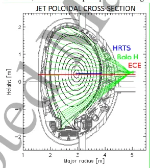
Concerning the profile of the electron temperature, both the ECE (Electron Cyclotron Emission) and the High-Resolution Thomson Scattering diagnostics [33] satisfy basic requirements to allow, in principle, the calculation of comparable peaking factors. JET ECE heterodyne radiometer consists of 96 channels over 4 data acquisition bands, allowing either first harmonic measurements (O-mode) or second harmonic measurements (X-mode) (see Figure 2). The High-Resolution Thomson Scattering (HRTS) diagnostic on JET measures electron temperature (Te) and electron density (Ne), providing 63 data points per profile with a repetition rate of 20 light pulses per second (20Hz) (see Figure 2). The spatial resolution of the measurements for the core region and the pedestal is respectively of 1.6 cm and 1 cm. Note that, HRTS has a lower time
resolution than the ECE signals. However, Te peaking factors based on the ECE diagnostic, in a not negligible
number of cases, were found to be affected by cut-off of several channels. The effect was sometimes marginal, other times was heavily jeopardizing the calculation of the peaking factor itself. Therefore, it was decided to replace ECE measurements with those of the HRTS, that in next JET campaigns is supposed to be available in real-time. In this first stage, it is indeed much more valuable to get correctly the overall picture of the parameter space where the relevant physics takes place rather than restricting the analysis with respect to real-time requirements. The same considerations apply also to other parameters that are introduced in the following, such as the safety factor on magnetic axis, for which the post-processed signals have been used.
Figure 2 – Sketch of the JET poloidal cross-section reporting the lines of sight of the main diagnostics used to derive the profile-based indicators discussed in the analysis: horizontal view bolometer camera (Bolo H) for radiation distribution,
Electron Cyclotron Emission (ECE) for Te radial profile and High-Resolution Thomson Scattering (HRTS) for Te and Ne
radial profiles.
Concerning the radiated power, the main-vessel bolometric camera with a horizontal view of the plasma cross-section (Bolo H) has been used. The camera collects the radiation along 24 chords, 8 of which in each case cross the divertor region and the region adjacent to the divertor with 8 cm separation between the chord axes. The other 16 channels cover the entire plasma. A simple pinhole structure is used to define the lines-of-sight of the camera [34]. 3 4 5 6 7 8 9 10 11 12 13 14 15 16 17 18 19 20 21 22 23 24 25 26 27 28 29 30 31 32 33 34 35 36 37 38 39 40 41 42 43 44 45 46 47 48 49 50 51 52 53 54 55 56 57 58 59 60
Accepted Manuscript
In [5], the peaking factors have been considered as features defined as a “core versus all” metric, i.e., they are defined as the ratio between the mean value of the considered radial profile (temperature, radiation, density) around the magnetic axis and the mean value of the measurements over the entire radius. The radial interval to define the “core” with respect to the magnetic axis has been empirically set to the 25% of the radial coordinate (the minor radius for poloidal mid-plane measurements) in the case of electron temperature and density profiles, and to the 10% of the vertical semi-axis of the poloidal cross section in the case of radiation profiles.
Regarding the peaking factor of the radiation, instead of considering a unique indicator to synthesize a peaking factor for the poloidal distribution of the radiation, as proposed in [5], two different indicators have been derived splitting the information carried out by the global radiation distribution according to the two main mechanisms involving a radiation collapse: the accumulation of high-Z impurities in the plasma core as opposed to edge-radiative collapse. As analyzed in [5], the main mechanisms with which the discharge is being destabilized are quite different, as well as the time scales involved in the corresponding chain of events. Nevertheless, although the initial version of the peaking factor was such that both the edge and core radiation collapse could be detected quite nicely, the two mechanisms are not mutually exclusive, and even if developing on different time scales, there are cases where both are simultaneously affecting the discharge.
As a general comment, even though in many cases it is possible to find “clean” examples of a well-defined chain of events corresponding to a specific disruption type, in other cases there is an interplay of more than one mechanism destabilizing the discharge, so that synthesizing more detailed and targeted indicators goes in the direction of a more accurate and flexible avoidance and prediction system.
Therefore, the information carried out by the peaking factor of the radiation profile is decomposed in two
separated indicators, one always based on the “core vs all metric” (Radpf-CVA) but having subtracted the
radiation in the X-point/divertor region, and the other one based on the “divertor vs all” (Radpf-XDIV) metric but
having subtracted the radiation in the core (decoupling in this way the contribution of the core radiation from the contribution of the divertor radiation). This has allowed in a sense, a decoupling of the two behaviors, improving at the same time the resolution of each of them.
To the five 1-D profile indicators (including the internal inductance as representative of the current density profile), other two dimensionless parameters have been integrated in the final dataset: the fraction of radiated
power with respect to the total input power (Pfrac) and the safety factor on magnetic axis (qAX). The first one is
a well-known indicator of the power balance. The second one is an important equilibrium parameter and, as
well-known from MHD stability theory, it is connected to the presence of the resonant surface for q=1 and the
sawtooth crashes due to the instability of the internal kink mode (m=1, n=1). This information, in connection
with the peakedness of the current profiles given by the internal inductance (Li), and the other parameters plays
a key role on the plasma stability as it will be described with some examples in the next sections. Table 1 lists the considered parameters.
Table 1. Plasma parameters
Parameter name Acronym
Peaking Factor of Temperature Tepf
Peaking Factor of Electron Density Nepf
Peaking Factor of the Radiation (excluding the contribution of the X-point/divertor region) Radpf-CVA
Peaking Factor of the Radiation (excluding the contribution of the core region) Radpf-XDIV
Internal Inductance Li
Fraction of the Radiated Power Pfrac
Safety Factor on magnetic axis qAX
As it will be discussed in the conclusions, some of these quantities might be affected by not negligible uncertainties in real-time processing. This preliminary step is needed to assess the feasibility of the approach that, at this first stage, has to be investigated separately from the uncertainties in real-time measurements.
3 4 5 6 7 8 9 10 11 12 13 14 15 16 17 18 19 20 21 22 23 24 25 26 27 28 29 30 31 32 33 34 35 36 37 38 39 40 41 42 43 44 45 46 47 48 49 50 51 52 53 54 55 56 57 58 59 60
Accepted Manuscript
The GTM models, as it will be described in the following sections, have been built using the flat top phase of non-disrupted discharges and the unstable phase of the disrupted discharges. This latter has been defined as
the phase after the time Ti, (identified as the start of the chain of events that is destabilizing the discharge), up
to the disruption time tD. For the considered discharges, these stable and unstable phases have been uniformly
sampled with a time step of 2ms.
Feature preprocessing
The selection of the discharges included in the database, both disruptions and regular terminations, has been carried out trying to preserve statistically the overall variety and variability of scenarios and experiments that
were carried out during the considered experimental campaigns. The main constraint, as described in [5], was
represented by the availability and the consistency of the signals needed to compute the features described in the previous section.
After the shot selection, the signals have been resampled with a uniform time step of 2 ms, which corresponds to the cycle time of the JET ATM network for real-time control. The basic preprocessing that has been performed takes into account real-time requirements, so that possible spikes and outliers are either discarded or smoothed out, by a causal median filtering of 40 ms width applied to each of the features. In fact, since the main objective of this work is to develop a tool for disruption avoidance, we are not interested in fast transient phenomena, but rather in destabilizing mechanisms that change the plasma state over longer time scales. A reasonable choice of the preprocessing parameters is a key element of an avoidance/prediction system to guarantee reliable detections and to avoid false alarms.
Then, a subsequent step, which is part of almost any machine learning workflow, consists of reducing the amount of data to be computationally manageable and also to overcome the classes’ unbalance that is due to longer stable phases of non-disrupted discharges with respect to the unstable phases of the disrupted ones. As previously cited, these phases have been uniformly resampled, so the non-disrupted space would be over represented with respect to the disrupted space.
Figure 3 – Probability Density Functions of Tepf, Pfrac, and Li, in arbitrary units [a.u.], before and after the data reduction for the non-disruptive space: the statistical distribution is preserved.
3 4 5 6 7 8 9 10 11 12 13 14 15 16 17 18 19 20 21 22 23 24 25 26 27 28 29 30 31 32 33 34 35 36 37 38 39 40 41 42 43 44 45 46 47 48 49 50 51 52 53 54 55 56 57 58 59 60
Accepted Manuscript
A GTM-based data reduction algorithm has been then applied shot by shot to the non-disrupted discharges reducing the number of samples by a prefixed factor. The data reduction algorithm allows to reproduce the same probability density function of the original data, as shown in Figure 3 that reports the probability density function of some of the input parameters of the original data set, on the top, and of the reduced set, on the bottom, using a reducing factor of nine. The same behavior has been found for all the other considered parameters. The peculiarity of preserving the probability distributions of high dimensional data is extremely important to avoid either the loss or the partial distortion of the statistical properties of the initial population and is not necessarily achieved by random under sampling.
IV.
Analysis of JET operational space with GTM
All the synthesized features have been used as input to build the GTM model. In order to test the generalization capability of the GTM model as disruption predictor, the data base has been split into two sets, a training set, which has been used to build the map, and a test set, to evaluate the prediction performance. The training set contains 89 disrupted shots and 70 regular terminations, whereas the test set is composed by 43 disruptions and 44 safe shots, which have never been presented to the model during the training. The selection of the training and test set has been performed in order to obtain two sets maximally independent and representative of the operational space. To this purpose, the test set contains discharges temporally subsequent to those in the training set. The different disruption classes are represented with the same percentage in the two sets, and repetition of discharges with same or similar setting are avoided.
A multi-objective Tabu Search (TS) [35] procedure has been customized to optimize the free parameters of
the GTM, i.e., the map dimension K, the number of radial basis functions M, and their width . The aim of the
optimization process is to maximize the log likelihood of the mapping of the training set, minimizing at the same time its sparsity, defined in terms of the percentage of empty clusters.
The TS is a metaheuristic method that looks for the optimal solution of an optimization problem by exploring the search space based on the use of adaptive memory. Starting from a random or a given initial point (described by the three free parameters of the GTM), at each iteration the algorithm explores all the neighbor points, selecting the best one. The TS strategy consists in exploring the search space along the coordinate directions (in this case each coordinate corresponds to a parameter of the GTM) and taking into account the most promising points to follow the search. TS avoids cycling by keeping in memory a list of examined points or their features so that the exploration of already investigated regions of the search space is inhibited and
stored in a Tabu List. The resulting optimal GTM has K=2500 latent points, and M=400 radial basis functions
with 𝜎 = 0.8, which correspond to a log likelihood of 9.85 ∙ 105 and a percentage of empty clusters of 12%,
obtained after 30 TS iterations. Note that, the stopping criteria was the maximum number of iterations (30 in our case). However, performing multiple independent TS runs with random initialization, except for the first few iterations, the others were non-improving ones.
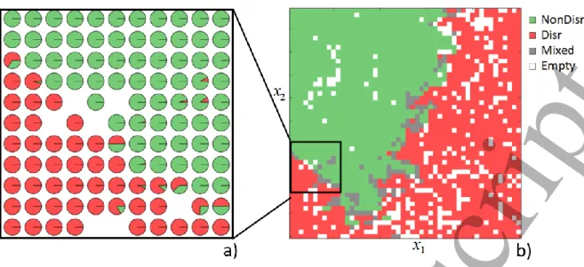
Figure 4 reports the 2-D GTM of the 7-D JET operational space corresponding to the feature set described in
the previous section, and obtained via DIS_tool. Figure 4-a reports the pie-plane representation, with reference
to the frame highlighted in Figure 4-b, of the mode of the posterior probability distribution over the latent space. Each node, or cluster, in the map represents the pie chart of the samples associated to that node. Green color refers to samples belonging to non-disruptive discharges, red color refers to samples coming from the unstable phase of the disrupted discharges. In Figure 4-b, each node in the map is colored depending on its composition: the green clusters contain only samples, the red clusters contain only samples (whereas grey clusters contain both non-disruptive and disruptive samples. The white clusters are empty. As can be seen, a well-defined separation between the two regions representing the disruptive (red) and non-disruptive (green) classes can be recognized in the 2-D latent space.
3 4 5 6 7 8 9 10 11 12 13 14 15 16 17 18 19 20 21 22 23 24 25 26 27 28 29 30 31 32 33 34 35 36 37 38 39 40 41 42 43 44 45 46 47 48 49 50 51 52 53 54 55 56 57 58 59 60
Accepted Manuscript
Figure 4 – GTM of the 7 plasma dimensionless parameters: (a) Pie plane representation (zoom of the frame selected in (b)) and (b) map colored on the basis of the node composition (each latent point is associated with a node in the 2D latent
space with coordinates x1 and x2 respectively. Note that, as usual for mappings onto a latent space, since the latent (hidden)
variables are arbitrarily normalized and do not carry on any direct information about the range of the input features, the coordinates values are not reported on the 2D map).
It can be seen how the operational spaces of the regular terminations and disruptions are well confined and quite compact; besides some isolated spots, there is only a narrow overlap on the boundary separating the two classes. This great separability of the two regions suggests the possibility to exploit with high-performance the obtained 2-D map as disruption predictor, as will be presented in the following Section V.
A further figure of merit to evaluate locally the degree of separation between classes is to analyze the composition of the clusters in the map. As can be seen by analyzing the map composition reported in Table 2, the degree of “separability” of disrupted and non-disrupted samples is quite high, the percentage of empty clusters is less than 12%, whereas the percentage of mixed clusters is less than 5%. The disrupted and non-disrupted clusters tend to aggregate according to the self-organization of the map that is driven only by similarities and differences in the probability density distribution of the input features. The unsupervised learning is shaping the 7-D input space in such a way that each of the two classes results to be predominant with respect to the other in different regions of the 2-D latent space. The optimal parameters give rise also to a quite low sparsity, suggesting that the size of the map with respect to the considered dataset is adequate.
Table 2. GTM composition
Type of cluster # clusters % clusters % samples in the clusters
% samples of a certain class belonging to clusters of the same
class Disrupted 1053 42.12 47.96 95.92 Non-disrupted 1045 41.80 47.21 94.42 Mixed 107 4.28 4.83 - Empty 295 11.8 - - 3 4 5 6 7 8 9 10 11 12 13 14 15 16 17 18 19 20 21 22 23 24 25 26 27 28 29 30 31 32 33 34 35 36 37 38 39 40 41 42 43 44 45 46 47 48 49 50 51 52 53 54 55 56 57 58 59 60
Accepted Manuscript
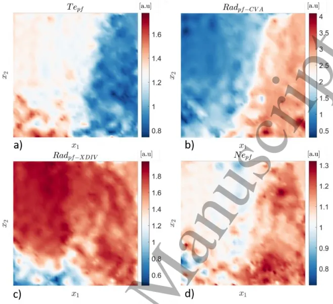
Figure 5 – Component plane representation of: (a) Peaking factor of the temperature (Tepf); (b) Peaking factor of the
radiation (Radpf-CVA); (c) Peaking factor of the radiation (Radpf-XDIV); (d) Peaking factor of the density (Nepf). The color
bars show the scale of the dimensionless variables.
Figure 5 and Figure 6 report the Component Planes that represent the relative component distributions of each of the input parameters used for the mapping. Component Planes distributions reflect univariate probability distribution (pdf) information uncovering patterns in the data. As discussed in [5], it can be seen that the individual features are already very descriptive of the different disruptive and non-disruptive behavior but what really makes the difference in the discrimination between the two spaces is how these parameters combine to capture the mechanisms destabilizing the discharge.
3 4 5 6 7 8 9 10 11 12 13 14 15 16 17 18 19 20 21 22 23 24 25 26 27 28 29 30 31 32 33 34 35 36 37 38 39 40 41 42 43 44 45 46 47 48 49 50 51 52 53 54 55 56 57 58 59 60
Accepted Manuscript
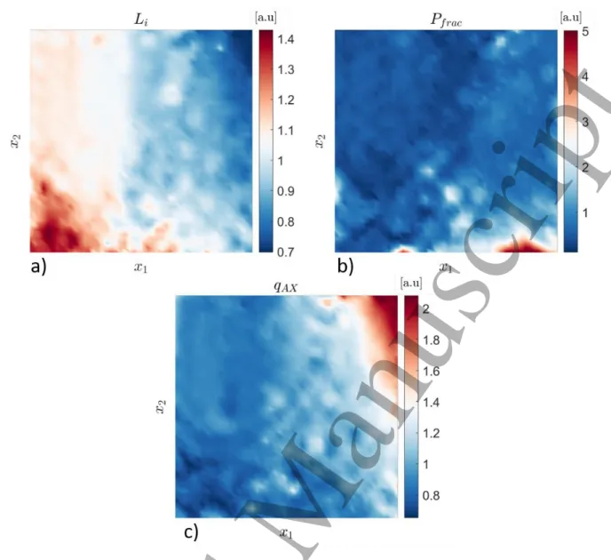
Figure 6 – Component plane representation of: (a) Internal Inductance (Li); (b) ratio of the total radiated power and the
total input power (Pfrac); (c) safety factor at the axis (qAX). The color bars show the scale of the dimensionless variables.
The basic interplay of radiation, kinetic and current density profiles have been already discussed in [5], whereas the contribution of the other components has been already described in the section dedicated to the feature construction. How each of the individual components resemble the shape highlighted in Figure 4 for the two classes depends on different factors. For instance, more than half of the disruptions composing the database are due to impurity accumulation and radiative collapse in the plasma core [18], [36], so that the distribution
of Radpf-CVA reflects quite closely the disruptive region for high values of this quantity. In this case, the
destabilizing mechanism is well described by such transition to higher values but is not the only ingredient and a fixed threshold is not enough for a reliable detection. The plasma response depends case by case by the plasma underlying conditions, the possible presence of other factors preventing, for instance, the full development of hollow temperature and current profiles. As can be seen by analyzing the component planes with respect to the regions occupied by the disruptive and non-disruptive samples, the patterns defined by the mapping cannot be easily extrapolated by considering individually the different features. The additional value of this machine learning approach is the capability to handle intrinsically the multivariate nature of complex operational spaces. This is extremely helpful for statistical analysis and visualization of the most recurrent patterns reflecting physics underlying mechanisms as well as for the interpretation of complex dependencies and relations among the different features.
As previously mention, the GTM is an unsupervised generative model, which aggregates the data, based on their probability density distributions. The map coloring used in this paper aims to highlight the discrimination
3 4 5 6 7 8 9 10 11 12 13 14 15 16 17 18 19 20 21 22 23 24 25 26 27 28 29 30 31 32 33 34 35 36 37 38 39 40 41 42 43 44 45 46 47 48 49 50 51 52 53 54 55 56 57 58 59 60
Accepted Manuscript
capability of the map in terms of classification between disrupted and non-disrupted space. Moreover, as shown in Figure 7, which is a different visualization of the GTM of Figure 4, the same boundary between disrupted and non-disrupted spaces is clearly visible both on the mode representation of the GTM in Figure 7 a), and in
the U-Matrix representation in Figure 7b). In the GTM tool [28] used in this paper, the like-Unified
Distance-Matrix (U-Distance-Matrix) plots the mean Euclidean distance between the barycenter of the samples of each cluster to its neighbors in a grayscale image. Macro regions of plasma states characterized by limited local variations are represented by lighter clusters and demarcated by darker clusters, which correspond instead to steeper local changes in the parameter space. This is consistent with the interpretation of the evolution of the plasma state significantly “deviating” during the transitions from a stable to an unstable phase. This result is particularly relevant since it has been obtained without any assumption a priori about the different nature of the two classes: it does represent an intrinsic property of the manifold where the data naturally lie. The correspondence of such intrinsic boundary separating the two regions corroborates the assumptions made with the manual selection of
the Reference Warning Times (Ref Ti).
Independently on the consistency in the selection of the warning times, one can wonder if a so clear separation and the resulting boundary are due to the global difference between non-disruptive and disruptive discharges rather than between the stable and the unstable phases. Therefore, in order to check how reliable the obtained boundary is, the non-disruptive discharges have been replaced by the stable phase of disruptions. Figure 8 a) reports the mode representation of the GTM obtained with only the disruptive discharges, whereas Figure 8 b) reports the corresponding U-Matrix. Note that, in this case, the obtained mapping is just representing the operational space of the disruptions.
As expected, the boundary is not as sharp as in the previous case and there is a larger overlapping because of the smoother transition between stable and unstable states but what is important to highlight here is that the boundary has still a similar shape. This is a clear indication that there is a common underlying structure characterizing the stable phases in the two cases. This is not obvious, and whether the “stable” phase of disruptive discharges is really close to that of non-disruptive discharges is still a debated point.
Figure 7 – (a) Mode representation (see paragraph Generative Topographic Mapping in section II) of the posterior probability distribution over the latent space for the GTM in Figure 4: green points refers to the regularly terminated discharges, whereas red points refers to the unstable phases of the disrupted discharges; (b) corresponding U-Matrix. The grey scale bar shows the value of the mean Euclidean distance between the barycenter of the samples of each cluster to its neighbors, from light grey to dark grey (from limited local variations to steeper local changes in the parameter space).
3 4 5 6 7 8 9 10 11 12 13 14 15 16 17 18 19 20 21 22 23 24 25 26 27 28 29 30 31 32 33 34 35 36 37 38 39 40 41 42 43 44 45 46 47 48 49 50 51 52 53 54 55 56 57 58 59 60
Accepted Manuscript
Figure 8 – (a) Mode representation of the GTM trained using only disrupted discharges: green clusters refer to the stable phases and red clusters refer to the unstable phases of the disrupted discharges; (b) corresponding U-Matrix. The grey scale bar shows the value of the mean Euclidean distance between the barycenter of the samples of each cluster to its neighbors, from light grey to dark grey (from limited local variations to steeper local changes in the parameter space).
V.
GTM for Disruption Avoidance
In this section, the potentialities of GTM mapping for the detection of a disruptive behavior early enough to enable avoidance actions are presented.
Tracking of the discharges on the GTM map
In addition to using the GTM map for operational boundaries studies, it can also be used for disruption prediction. In fact, the potentiality of the available toolbox for the GTM [28] allows us to track the temporal sequence of the samples on the map, depicting the movement of the operating point during a discharge. Following the trajectory on the map, it is possible to eventually recognize the proximity to an operational region where the risk of an imminent disruption is high. Based on such GTM information, an alarm would be triggered as will be described in the next subsection. In this work, furthermore, the alarm provided by the pure
GTM tracking (GTM7) will be studied also in combination with the detection of MHD modes locking
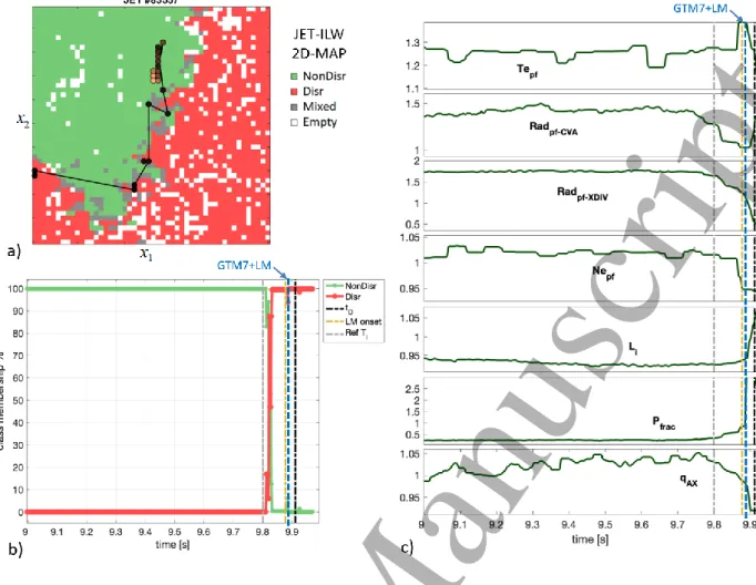
(GTM7+LM), analyzing the different contributions with respect to the involved time scales. In Figure 9 a), the
trajectory of the JET disrupted discharge #82657 is reported, where a gradually changing color scale is used to show the temporal evolution of the discharge, from the lighter in the beginning of the discharge to the darker point that corresponds to the disruption time. As it can be noted, the disruptive discharge starts in a non-disruptive cluster, firstly evolving in the stable (green) region, enters the unstable (red) region, ending in a disruptive cluster, which corresponds to the disruption time. Note that, because of the profile-based indicators defined for the analysis, all the discharges have been projected on the map for the entire time interval of the
flat-top phase (up to the disruption time tD in case of disruptions) where the plasma is in the X-point
configuration. In the following, the initial time has been named T0.
The evolution of the discharge on the map can be better visualized referring to the class membership function
shown in Figure 9b). The class membership function is defined with respect to the composition of the clusters
where the operative point is evolving. In particular, it represents the percentage of samples of the considered class in the cluster to which the sample is associated, with respect to the total number of samples in the cluster itself. The experiment referred in Figure 9, performed for fueling and impurity seeding studies with Neon, is characterized by an initial significant Tungsten event at ~13.5s, which perturbs temporarily the seven parameters provided as input to the GTM (Figure 9 c)). After that, the plasma recovers completely up to a
3 4 5 6 7 8 9 10 11 12 13 14 15 16 17 18 19 20 21 22 23 24 25 26 27 28 29 30 31 32 33 34 35 36 37 38 39 40 41 42 43 44 45 46 47 48 49 50 51 52 53 54 55 56 57 58 59 60
Accepted Manuscript
second Tungsten event, which again perturbs the parameter space, causing this time a more significant transition in the class membership functions up to the large influx of W, together with other impurities, in
correspondence to the reference warning time Ref Ti, that is slightly before 18s. This latter represents “the point
of no return”, after which the plasma is definitely destabilized, and we can observe the typical signatures of an impurity accumulation process, with the sawtooth activity stopping and the accumulation of several impurities building up in the plasma core. Because of the strong radiation from the core, as clearly showed by the radiation peaking, the temperature and the current profiles become hollow, as reflected by the temperature peaking factor
(Tepf) and the internal inductance (Li) time evolutions. This condition, where the plasma confinement is already
deteriorated, evolves until the locking of an MHD instability, a (m=2, n=1) mode, which eventually triggers
the disruption.
Figure 9 – a) Projection of the disrupted discharge # 82657 on the GTM of Figure 4. The lighter points correspond to the
beginning of the discharge, whereas the darker one corresponds to the end, at the disruption time tD; b) Class member
functions of non-disrupted (green) and disrupted (red) classes; c) Time evolution of the 7 plasma parameters used to build the GTM. The vertical dashed lines in b) and c) correspond to specific times of interest characterizing the evolution of
the discharge: the time of influx of W and other impurities, Imp. Influx (purple), the Reference Warning Time, Ref Ti, i.e.
the time indicative of the start of the chain of events leading to disruption that has been manually identified (overlapping with the third impurity influx, indicated by a grey arrow); the time where the prediction system would trigger an alarm,
GTM7+LM (blue); the time of the locked mode onset, LM onset (yellow); the disruption time, tD (black).
As can be noted, the disruption precursors caught by the peaking factors appear well in advance with respect to the onset of the locked mode, corroborating the chance of using these features for a much earlier detection of a disruptive behavior, which is an essential requirement for any action of avoidance.
3 4 5 6 7 8 9 10 11 12 13 14 15 16 17 18 19 20 21 22 23 24 25 26 27 28 29 30 31 32 33 34 35 36 37 38 39 40 41 42 43 44 45 46 47 48 49 50 51 52 53 54 55 56 57 58 59 60
Accepted Manuscript
Figure 10 – a) Projection of the non-disrupted discharge # 83852 on the GTM of Figure 4. The color of the circle depicting the movement of the operating point becomes darker and darker as the discharge is approaching to the final phase; b) Class member functions of non-disrupted (green) and disrupted (red) classes.
In Figure 10, the trajectory of the regularly terminated discharge #83852 is reported. As in the majority of the regularly terminated discharges, during the flat-top (FT) phase of the plasma current the non-disrupted discharge trajectory typically evolves within the green “stable” region. It can be noted that in the final ramp-up and in the early ramp-down phases the class-membership functions are slightly perturbed because of the rapidly varying parameters. In this case, the map, beyond the aforementioned “spikey” transitions, is clearly recognizing the non-disrupted nature of the plasma. Any significant change or transition in the plasma state is reflected to some extent in the evolution of the operating point, shifting sometimes the trajectory towards the boundary separating the non-disruptive from the disruptive region on the map. During the time evolution of regular terminations as well as during the stable phases of disruptive discharges, such transitions are mostly localized within the boundary or in a quite narrow layer across the boundary separating the stable from the unstable phases.
Trigger functions and alarm handling
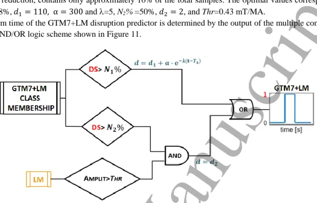
As previously described, following the trajectory on the map throughout the different regions, it is possible to recognize plasma configurations with different risk of disruption. In order to trigger an alarm, a simple criterion has been optimized, which links the disruption risk of the map clusters to the percentage of disrupted samples into the clusters. Moreover, in order to limit possible tardy or missed alarms due to disruptive processes characterized by fast time scales, or false alarms due to transients, the multiple conditions alarm scheme reported in Figure 11 has been implemented to handle the activation of an alarm. In particular, the condition derived from the GTM model is that an alarm is triggered when the trajectory stays in a disruptive or a mixed
cluster containing a percentage of disruptive samples DS>N1% for at least 𝑑 consecutive samples. Note that
for our specific application, a sample corresponds to a time unit of 2ms, that is the cycle time of the JET
real-time network (ATM). The total assertion time𝑑 has been assumed to vary with the time evolution of the
discharge with the following exponential law:
𝑑 = 𝑑1+ α ∙ e−λ(t−𝑇0)
where T0 is the time when the plasma assumes the X-point configuration. Conversely, if the operating point
lays in a mixed cluster with a percentage of disruptive samples N2%<DS<N1%, also the Locked Mode
amplitude signal, normalized with respect to the plasma current, is considered to trigger the alarm, and a fixed
value of the assertion time 𝑑2 is assumed. In order to avoid overfitting and maximize the GTM model capability
to generalize, the alarm criteria parameters N1%, 𝑑1, α, , and N2%, 𝑑2, as well as the threshold Thr [mT/MA]
3 4 5 6 7 8 9 10 11 12 13 14 15 16 17 18 19 20 21 22 23 24 25 26 27 28 29 30 31 32 33 34 35 36 37 38 39 40 41 42 43 44 45 46 47 48 49 50 51 52 53 54 55 56 57 58 59 60
Accepted Manuscript
on the Locked Mode amplitude, have been chosen by optimizing the total prediction error of the GTM on a cross validation set composed by all the training discharges. Note that, this set is completely independent from the set used to train the GTM model as far as the stable phase of disruptive discharges is concerned, whereas, regarding their unstable phase and the whole phase of non-disruptive discharges, the training set, because of the data reduction, contains only approximately 10% of the total samples. The optimal values correspond to
N1% =98%, 𝑑1= 110, α = 300 and =5, N2% =50%, 𝑑2= 2, and Thr=0.43 mT/MA.
The alarm time of the GTM7+LM disruption predictor is determined by the output of the multiple conditions in the AND/OR logic scheme shown in Figure 11.
Figure 11 – Multiple condition alarm scheme of the GTM7+LM disruption predictor.
In Figure 12 an example of disruption occurring with a quite fast time scale is shown. The stationarity of the discharge is firstly destabilized by a W event at ~9.8s, followed by an influx of low Z impurities, which through
the cooling of the plasma edge leads to the locking of the (m=2, n=1) mode. In this case, the alarm is triggered
by the bottom branch in input to the OR logic in the scheme of Figure 11, which is reacting before the top
branch. This is a situation occurring mostly when the disruptive process develops on relatively short time
scales such that the effect on the 7-D features space, also because of their processing and the assertion time d,
propagates later than the detection of the Locked Mode. Nevertheless, it is worth to note that also in this case there is a well-defined transition in the class-membership functions before the mode locking, with the operating point approaching the boundary between the two classes on the map shortly after the impurity event.
3 4 5 6 7 8 9 10 11 12 13 14 15 16 17 18 19 20 21 22 23 24 25 26 27 28 29 30 31 32 33 34 35 36 37 38 39 40 41 42 43 44 45 46 47 48 49 50 51 52 53 54 55 56 57 58 59 60
Accepted Manuscript
Figure 12 – a) Projection of the final phase of the disruptive discharge # 83557 on the GTM of Figure 4. The color of the circles depicting the evolution in time of the operating point becomes darker and darker as the discharge is approaching to the final phase; b) Class member functions of the non-disrupted (green) and disrupted (red) classes; c) Time evolution of the 7 plasma parameters used to build the GTM. The vertical dashed lines in b) and c) correspond to
specific times of interest characterizing the evolution of the discharge: the Reference Warning Time, Ref Ti (grey); the
time where the prediction system would trigger an alarm, GTM7+LM (blue); the time of the Locked Mode onset, LM
onset (yellow); the disruption time, tD (black).
Performance of the GTM as Disruption predictor
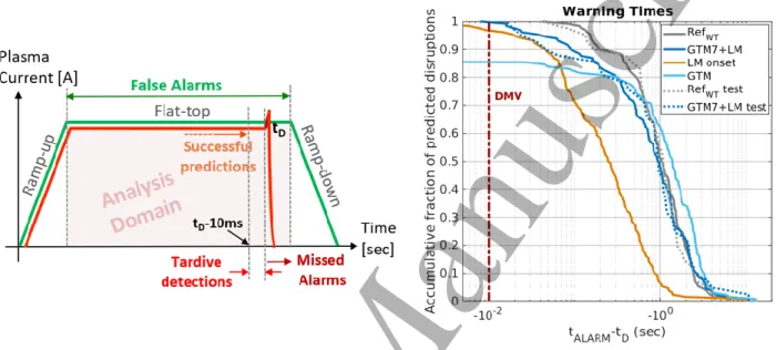
According to the literature, the performance of the proposed disruption prediction system is evaluated in terms of successful predictions on disruptions (SPs), missed alarms (MAs), tardy detections (TDs) (a detection is considered tardy if the warning time is less than 10 ms), and false alarms (FAs). A sketch to summarize the aforementioned definitions is reported in Figure 13 a). Since the main aim of the present system is the avoidance of disruptions, premature detections are not included in the present analysis, but they will be discussed in the next section. The purpose here is to obtain a distribution of the actual warning times as close
as possible to the Reference Warning Times Ref Ti, evaluated with respect to the start of the chain of events
leading to the disruptions and identified manually.
The performances on the discharges both in the test and in the training set have been evaluated resulting in all correct predictions but one tardive detection (in the training set) and 7 false detections (6%), 3 over the training and 4 over the test datasets. Regarding the “false” detections in regularly terminated discharges, a more in-depth reasoning needs to be done, and this is postponed to the next section about the analysis of the results. This very good performance is associated to a quite early detection of a disruptive behavior, as shown in Figure 13 b), which reports the cumulative warning time distribution of the proposed GTM7+LM predictor (in blue), evaluated as the difference between disruption time and GTM7+LM alarm time. A second cumulative
3 4 5 6 7 8 9 10 11 12 13 14 15 16 17 18 19 20 21 22 23 24 25 26 27 28 29 30 31 32 33 34 35 36 37 38 39 40 41 42 43 44 45 46 47 48 49 50 51 52 53 54 55 56 57 58 59 60
![Figure 3 – Probability Density Functions of Te pf , P frac , and L i , in arbitrary units [a.u.], before and after the data reduction for the non-disruptive space: the statistical distribution is preserved](https://thumb-us.123doks.com/thumbv2/123dok_us/1918334.2781885/12.892.212.686.698.1089/probability-functions-arbitrary-reduction-disruptive-statistical-distribution-preserved.webp)