Is forecasting with large models informative? Assessing the role of judgement in macroeconomic forecasts

Working PaPer SerieS

no 950 / oCToBer 2008

iS ForeCaSTing WiTh

Large ModeLS

inForMaTive?

aSSeSSing The roLe

oF judgeMenT in

ForeCaSTS

by Ricardo Mestre

and Peter McAdam

In 2008 all ECB publications feature a motif taken from the 10 banknote.

W O R K I N G PA P E R S E R I E S

N O 9 5 0 / O C T O B E R 2 0 0 8

IS FORECASTING WITH LARGE

MODELS INFORMATIVE?

ASSESSING THE ROLE OF

FORECASTS

by Ricardo Mestre

_{and Peter McAdam}

This paper can be downloaded without charge from http://www.ecb.europa.eu or from the Social Science Research Network electronic library at http://ssrn.com/abstract_id=1284926.

1 The views expressed in this paper do not necessarily reflect the views of the European Central Bank. 2 Corresponding author: European Central Bank, DG Research, Kaiserstrasse 29, D-60311

JUDGEMENT IN MACROECONOMIC

© European Central Bank, 2008 Address

Kaiserstrasse 29

60311 Frankfurt am Main, Germany Postal address

Postfach 16 03 19

60066 Frankfurt am Main, Germany Telephone +49 69 1344 0 Website http://www.ecb.europa.eu Fax +49 69 1344 6000 All rights reserved.

Any reproduction, publication and reprint in the form of a different publication, whether printed or produced electronically, in whole or in part, is permitted only with the explicit written authorisation of the ECB or the author(s).

The views expressed in this paper do not necessarily refl ect those of the European Central Bank.

The statement of purpose for the ECB Working Paper Series is available from the ECB website, http://www.ecb.europa. eu/pub/scientific/wps/date/html/index. en.html

ISSN 1561-0810 (print) ISSN 1725-2806 (online)

CONTENTS

Abstract 4

Non-technical summary 5

Introduction 7

1 Analysis of the RMSE of the forecasts 9

1.1 Pitfalls in forecasting 9

1.2 The framework 9

1.3 A RMSE decomposition 10

2 The AWM: data and specifi cation 12

3 Description of the exercise 14

3.1 The forecasting steps 15

3.2 Treatment of additional exogenous

information 16

3.3 Treatment of residuals 16

3.4 Re-estimation procedure 18

3.5 Alternative benchmark models 19

4 Results 19

4.1 Simulated out-of-sample exercise 20

4.2 In-sample exercise 21

4.3 Forecasting in EMU 23

4.4 Further exercises on infl ation trends 24

5 Conclusions 25

Acknowledgements 27

References 28

Tables and fi gures 29

Annexes 41

Abstract

We evaluate residual projection strategies in the context of a large-scale

macro model of the euro area and smaller benchmark time-series models. The

exercises attempt to measure the accuracy of model-based forecasts simulated

both out-of-sample and in-sample. Both exercises incorporate alternative

residual-projection methods, to assess the importance of unaccounted-for

breaks in forecast accuracy and off-model judgment. Conclusions reached are

that simple mechanical residual adjustments have a significant impact of

forecasting accuracy irrespective of the model in use, ostensibly due to the

presence of breaks in trends in the data. The testing procedure and

conclusions are applicable to a wide class of models and thus of general

interest.

Keywords: Macro-model, Forecast Projections, Out-of-Sample, In-Sample, Forecast Accuracy, Structural Break.

NON-TECHNICAL SUMMARY

Is forecasting with large models useful? The question is far from trivial, since most macro-models fulfil two (essentially conflicting) purposes: that of offering ‘good’ forecasts and at the same time ‘good’ stories. The first goal in a forecasting institution is clear. The second, though less conspicuous, is equally important since stories are used by staff preparing the forecast to assess their degree of mutual understanding of the resulting numbers. Stories are also needed to impress upon the public the degree of thoughtfulness and quality in the forecast. Policy-making is also about shaping expectations, and these cannot be properly handled if the forecast is presented only in terms of how well it fits past data. Stories are part of policy communication, and hence part of the credibility toolbox of policy institutions.

The alternatives to macro-models are time-series-based ones, usually of relative smaller sizes but with good fitting and forecasting properties. These models may be less apt at the business of ‘building’ stories, but have become the de-facto benchmarks in forecasting contests, see Stock and Watson (1999), Marcellino et al. (2003), McAdam and McNelis (2005). Accordingly, we shall use them as such here alongside forecasting exercises on a large macro-model.

Broadly speaking, macro-models try to capture two different economic facts: long-run static economic relationships and the dynamics inherent in the data. The two are oftentimes handled differently, with many models including a rigorous description of the steady-state that is sometimes at odds with the historic data; and dynamic mechanisms that frequently fit the data considerably better. That this is so is no coincidence: traditionally, models are made to fit the data through modelled dynamics and are made to tell stories through their modelled economic structure. The European Central Bank’s model, the Area-Wide Model (AWM), is such an example with a number of features of particular interest for the task at hand. First, it has a rich steady-state embedded in it, whose complexity lies more in the fact that steady-state conditions are endogenous rather then its sheer size. Second, it has almost-freely estimated dynamics, which ensures a degree of congruence with the business-cycle properties of the data. In short, a perfect workhorse for the forecasting exercise we plan.

However, one less well understood (or communicated) issue in the context of model-based forecasting is the trade off between “free” model-based forecasting and “judgment”. Often model-based forecasters employ judgment (i.e., shifting the residuals of behavioural equations) to impose paths that reflect some missing feature of the model (e.g., confidence effects, omitted variables); remedy some known deficiency of the model (e.g., unsatisfactory dynamics); or impose information on some sufficiently large idiosyncratic shocks (e.g., labour strikes) or off-model expert judgment (e.g., leading indicators, “flash” estimates). The imposition of judgment over an entire forecast round may reflect each or all of these or simply indicate institutional practices (such as initializing a new forecast with the previously-imposed judgment). Consequently judgment can turn out to be as or more important than traditionally-studied aspects of forecast uncertainty (e.g., parameter, specification uncertainty).

Given this, it may be considered peculiar (if not alarming) that the “black arts” of judgment strategies (e.g. their form, strengths, weakness, justification) are rarely brought to light. The purpose of this paper therefore is to shed light on the impact and interpretation of judgment on forecast accuracy; in short, to shine some hard science on these black arts. Of course, an all-encompassing analysis of residual projection strategies is a complex (and often highly model-/user- specific) task whose full analysis necessarily lies beyond our scope. We target a more tractable, constructive goal: to assess how shifts based on plausible laws of motion which capture off-model judgment end up affecting forecasts, particularly at long horizons.

The analysis has been carried out using two different versions of the AWM: the original model, as specified and estimated originally, and the same model with the addition of equations for the most important exogenous variables from a Structural Vector Auto-Regression Model (SVAR). Both were used to simulate out-of-sample and in-sample forecasts using the original estimation dataset, and an updated and revised dataset. Projections with the AWM were then benchmarked against alternative time-series-based models. Furthermore, the AWM model was subjected to a simple set of plausible yet informative strategies to project residuals, to analyze the impact of off-model information. When using the revised dataset, the alternative models were also subjected to the preferred residual-projection strategy, based on shifting residuals according to their mean over the preceding four periods. Using a decomposition of the Root Mean Square Error metric, we judge the dimensions in which different models and residual projection strategies succeed.

Based on projections for GDP growth, GDP deflator inflation and consumption deflator inflation, we conclude: the AWM (which can be taken as an example of a large model) is neither particularly hampered nor helped by its size when producing forecasts. Furthermore, many of the issues found using the model are also present in smaller, time-series-based models. Taking each variable in turn: for GDP growth, residual shifting helps in reducing forecast bias to some extent, but the increase in forecast variance brought by the method more than outweighs those gains; for inflation, bias reduction is often sufficiently important to actually improve outcomes. This result holds for most models used, foremost among them the AWM. Our understanding of these findings is that GDP growth may have been slightly higher on average in the estimation sample compared with the forecast sample, but was otherwise not strongly affected by breaks,

while inflation was more fundamentally affected by breaks between the two samples.1 _{The exercise is}

compatible with a declining trend in inflation over the estimation period and its absence in the forecast period. Unless the trend in inflation is successfully modelled, the only way to forecast inflation with some success is by using models that, while being potentially different from the data-generation process, are robust to changes in trends. To empirically assess the point, the forecasting performance of simple AR

models of 1st_{-differences of inflation (i.e., over-differencing) is checked and found to outperform the}

preferred in-sample model.

Introduction

Is forecasting with large models useful? The question is far from trivial, since most macro-models fulfil two (essentially conflicting) purposes: that of offering ‘good’ forecasts and at the same time ‘good’ stories. The first goal in a forecasting institution is clear. The second, though less conspicuous, is equally important since stories are used by staff preparing the forecast to assess their degree of mutual understanding of the resulting numbers. Stories are also needed to impress upon the public the degree of thoughtfulness and quality in the forecast. Policy-making is also about shaping expectations, and these cannot be properly handled if the forecast is presented only in terms of how well it fits past data. Stories are part of policy communication, and hence part of the credibility toolbox of policy institutions.

The alternatives to macro-models are time-series-based ones, usually of relative smaller sizes but with good fitting and forecasting properties. These models may be less apt at the business of ‘building’ stories, but have become the de-facto benchmarks in forecasting contests, see Stock and Watson (1999), Marcellino et al. (2003), McAdam and McNelis (2005). Accordingly, we shall use them as such here alongside forecasting exercises on a large macro-model.

Broadly speaking, macro-models try to capture two different economic facts: long-run static economic relationships and the dynamics inherent in the data. The two are oftentimes handled differently, with many models including a rigorous description of the steady-state that is sometimes at odds with the historic data; and dynamic mechanisms that frequently fit the data considerably better. That this is so is no coincidence: traditionally, models are made to fit the data through modelled dynamics and are made to tell stories through their modelled economic structure. The European Central Bank’s model, the Area-Wide Model (AWM), is such an example with a number of features of particular interest for the task at hand. First, it has a rich steady-state embedded in it, whose complexity lies more in the fact that steady-state conditions are endogenous rather then its sheer size. Second, it has almost-freely estimated dynamics, which ensures a degree of congruence with the business-cycle properties of the data. In short, a perfect workhorse for the forecasting exercise we plan.

However, one less well understood (or communicated) issue in the context of model-based forecasting is the trade off between “free” model-based forecasting and “judgment”. Often model-based forecasters employ judgment (i.e., shifting the residuals of behavioural equations) to impose paths that reflect some missing feature of the model (e.g., confidence effects, omitted variables); remedy some known deficiency of the model (e.g., unsatisfactory dynamics); or impose information on some sufficiently large idiosyncratic shocks (e.g., labour strikes) or off-model expert judgment (e.g., leading indicators, “flash” estimates). The imposition of judgment over an entire forecast round may reflect each or all of these or simply indicate institutional practices (such as initializing a new forecast with the previously-imposed judgment). Consequently judgment can turn out to be as or more important than traditionally-studied aspects of forecast uncertainty (e.g., parameter, specification uncertainty).

Given this, it may be considered peculiar (if not alarming) that the “black arts” of judgment strategies (e.g. their form, strengths, weakness, justification) are rarely brought to light. The purpose of this paper therefore is to shed light on the impact and interpretation of judgment on forecast accuracy; in short, to shine some hard science on these black arts. Of course, an all-encompassing analysis of residual projection strategies is a complex (and often highly model-/user- specific) task whose full analysis necessarily lies beyond our scope. We target a more tractable, constructive goal: to assess how shifts based on plausible laws of motion which capture off-model judgment end up affecting forecasts, particularly at long horizons.

The analysis has been carried out using two different versions of the AWM: the original model, as specified and estimated originally, and the same model with the addition of equations for the most important exogenous variables from a Structural Vector Auto-Regression Model (SVAR). Both were used to simulate out-of-sample and in-sample forecasts using the original estimation dataset, and an updated and revised dataset. Projections with the AWM were then benchmarked against alternative time-series-based models. Furthermore, the AWM model was subjected to a simple set of plausible yet informative strategies to project residuals, to analyze the impact of off-model information. When using the revised dataset, the alternative models were also subjected to the preferred residual-projection strategy, based on shifting residuals according to their mean over the preceding four periods. Using a decomposition of the Root Mean Square Error metric, we judge the dimensions in which different models and residual projection strategies succeed.

Based on projections for GDP growth, GDP deflator inflation and consumption deflator inflation, we conclude: the AWM (which can be taken as an example of a large model) is neither particularly hampered nor helped by its size when producing forecasts. Furthermore, many of the issues found using the model are also present in smaller, time-series-based models. Taking each variable in turn: for GDP growth, residual shifting helps in reducing forecast bias to some extent, but the increase in forecast variance brought by the method more than outweighs those gains; for inflation, bias reduction is often sufficiently important to actually improve outcomes. This result holds for most models used, foremost among them the AWM. Our understanding of these findings is that GDP growth may have been slightly higher on average in the estimation sample compared with the forecast sample, but was otherwise not strongly affected by breaks,

while inflation was more fundamentally affected by breaks between the two samples.2 _{The exercise is}

compatible with a declining trend in inflation over the estimation period and its absence in the forecast period. Unless the trend in inflation is successfully modelled, the only way to forecast inflation with some success is by using models that, while being potentially different from the data-generation process, are robust to changes in trends. To empirically assess the point, the forecasting performance of simple AR

models of 1st_{-differences of inflation (i.e., over-differencing) is checked and found to outperform the}

preferred in-sample model.

The paper proceeds as follows: Section 2 motivates the forecasting exercise; Section 3 briefly discusses the Area Wide Model; Section 4 analyses the consequences for model-based projection exercises given

different residual projection strategies in the context of the AWM, whilst section 5 presents the empirical results. Finally, we conclude.

1.

Analysis of the RMSE of the forecasts

1.1 Pitfalls in Forecasting

Hendry and Clements (1998, 1999) propose a taxonomy of potential causes for forecast failure including:

i) In-sample model mis-specification or data-based model selection;

ii) Poor estimation strategies or incorrect calculation of confidence intervals;

iii) Parameters depending on policy-regime changes;

iv) Structural un-forecastable breaks, also called deterministic shifts.

To different degrees, all these factors are worth exploring in our analysis. Points i) and ii) will be assessed by making use of alternative models to the AWM for benchmarking. Point iii) will be tackled by assessing the degree of parameter instability in the model by re-estimating the model with an artificially expanding sample. Point iv) will be assessed by suitable alternative residual adjustment and projection methods, with the goal in mind of replicating un-modelled changes in trends.

1.2 The Framework

Simple residual-projection strategies will be adopted: from projections in which residuals will be set to their in-sample average (normally around zero) to more sophisticated rules. Some of these strategies affect the steady-state of the model by causing deterministic shifts. A statistical framework is needed to assess their effects and understand the methodological approach taken. Let us thus assume that variables to be forecast (e.g., output growth, inflation) are stationary. A Wold decomposition for them can then be found, see

expression (1): variable xt is decomposed into a deterministic time-varying component μt and a stationary

moving-average of possibly infinite dimension of the process İt, itself stationary and independently

distributed. Assume (1) represents the true data generation process of the variable to be forecast, and is thus unknowable. Forecasts will be based on models that (hopefully) approximate process (1) but will in general differ in one aspect or another from it. Expression (2) expresses the forecasting models, again in the form of a Wold decomposition. f f ˜ _{, where}

¦

V

H

T

P

H

T

¦

V

K

M

Q

K

M

Forecasts with the models are as in (3), in which f_th is a stochastic forecast obtained from (2) h steps ahead. The error process in the forecast period is assumed to be given by a deterministic rule (such as e.g.

, for t belonging to the forecast horizon). It is important to stress that forecasts are stochastic because

of their conditioning on past information, itself stochastic, not because stochastic simulations will be run with the models. The fact that residual projection is deterministic means that the forecasts will sooner or later converge to a deterministic process with unit probability.

0 h t

K

^

`

>

@

> @

One important aspect of the comparison between (1) and (2) is that they can be used to formalize some potentially important sources of forecast failure. Namely, there could be a false description of trends on the

one hand (

P Q

(

T

M

former could have a much longer-lasting influence. In what follows, strategies to project residuals will be explicitly linked to the sources of forecast failure tackled in each case.

Note that the taxonomy of forecast errors described is better used with models whose dynamics are well adapted to the intrinsic dynamics in the data. If instead the dynamics in the model are strongly

mis-specified3, identifying un-forecastable breaks is significantly more challenging, as errors in forecasting

trended behaviour and dynamics get blended. It is true that errors in the modelled dynamics will only affect forecast accuracy in the short- to medium-run, but the relatively short samples used in the paper may be insufficient to offset the effects of badly-modelled dynamics. Some care will thus be taken in modelling properly the dynamics of all the models. We are now in a position to understand how forecast errors will be analyzed.

1.3 A RMSE Decomposition

Assuming that an h-step-ahead forecast f_th is generated using (3), the measures of accuracy of forecast

used in the preceding sections are given by the MSE (Mean Square Error) as in (4). Reported Root Mean Square Errors (RMSEs) are simply their root. In the expression, abusing notation, the expectation is made

conditional on information previous to the start of the forecast at T.

The expression for MSE leads naturally to a decomposition of the statistic using the Wold decomposition of

actual and forecast. Taking into account that

>

@

t t h t h t t t h t t f x f x ( P Q P Q ( ,

f Q , it is easy to show that expression (4) is equivalent to (5), which itself

can be rewritten as (6):

3 _{This could result from the imperfect modeling of those dynamics or from an explicit choice by the model builder to represent the}

>

@

P

Q

P

Q

P

Q

t var var 2 cov , bias

MSE ˜ h t t h t t f x f x (6)

This expression is interesting because it decomposes the MSE along components about some of which we can a priori say something. Namely, the distributional assumptions made means that the first element is given and outside the control of the analyst. The only hope to reduce forecast error is by ensuring that: i) no bias is introduced in the forecast and ii) the variance of the forecast error, itself depending on the variance of the forecast and the covariance between actual values and forecasts, is small. Note that point ii) will give

ceteris paribus the advantage to models in which var h t

f is small, irrespective of whether the models fit

the data well. For instance, a forecast fixed at some value for all periods may be completely uncorrelated with the actual realizations, but its null forecast variance may turn this into a powerful forecasting strategy. The trade-off between forecast variability, its correlation with actual observations and the presence of biases may mean that ‘wrong’ models may provide smaller forecast RMSE.

Furthermore, if the forecast procedure is deterministic (i.e., var

K

the variance of the forecast will shrink as the forecast horizon is increased, as shown below,

V

M

K

M

K

M

K

M

K

M

Q

¦

¦

¦

¦

Hence, lim var _th 0, which means that

hof f plim

h t

f

Q

h

o

f

phenomenon applies to the covariance between actual and forecast outcomes. This means that in (6)all the elements except the first and last ones converge to zero as the forecast horizon is increased. The obvious implication is that, in long-horizon forecasts, avoiding biases is the only thing that matters. It is interesting to find whether a sample counterpart to (6) can be found, in order to assess the relative importance of all these factors. Unfortunately, this can be achieved only at some cost.

The sample expression for the MSE is given by (8), where it is assumed that the first forecast is done at time

0 and that the variable xt spans until period T and is assumed to be present for at least h periods before time

0. A natural extension to express the MSE decomposition as in (6) would be to replace variances and means in the expression by their sample counterparts, as in (9). This expression, though, relies on the assumption

that means do not depend on t, i.e. that

P

P Q

Q

may be disadvantaged by our choice, since in their case var h t

f may not decrease at all as h increases.4

We will nevertheless use (9) to decompose shown MSEs, in the conviction that such decomposition can lead to interesting insights.

¦

¦

¦

¦

¦

¦

2.

The AWM: Data and Specification

The AWM treats the euro area as a single economy. Its structure is standard, having a long-run classical equilibrium with a vertical Phillips curve but with some short-run frictions in price/wage setting, factor demands, etc. Consequently, activity is determined in the short run by demand – given incomplete nominal adjustment – but is determined by supply in the longer run, with employment having converged to a level consistent with the exogenously given level of equilibrium unemployment (the NAIRU). In addition, stock-flow adjustments are accounted for, e.g. by the inclusion of a wealth / cumulated saving term in consumption or an explicit net foreign assets accumulation mechanism. With the exception of the forward-looking exchange rate (modelled by uncovered interest parity, UIP) the model embodies adaptive expectations.

The AWM is estimated using the European Central Bank’s area-wide database which has been widely used:

inter alia, Coenen and Vega (2001), Galȓ et al. (2001), Smets and Wouters (2003), Marcellino et al. (2003),

McAdam and Willman (2004). Applications of the model itself include examining the performance of policy rules and the monetary transmission mechanism (Adalid et al. 2005; McAdam and Morgan, 2002), policy making under a zero lower bound nominal interest rate constraint (Dieppe and McAdam, 2006), the determination of real exchange-rate paths (Detken et al. 2002), etc.

The model will be taken broadly as originally estimated, i.e. using at the time a dataset that went until around 1998Q4. Two databases have been used in the paper: initially, a simple update of the original dataset until 1999Q4; second, a much deeper revision of the dataset until 2006Q4. The latter dataset differs from the original one in many respects: the most recent periods are chain-linked data from Eurostat and most

4 _{For instance, ranking of models based on their RMSE in forecasting inflation may change if changes in sample inflation means are}

backdates come from the SNA93 revision of the OECD. Furthermore, some series have changed their definition, such as for instance a different split between private and Government consumption. All this adds up to a very significant change in the data. The analysis has been carried out using the original dataset to avoid (to the extent possible) contamination of deterministic and stochastic sources of forecast error, as the dynamics in the AWM were fine-tuned to this specific dataset. The updated dataset is used to report an enlarged set of results.

It remains to link the use of the model with the discussion on changing trends, point iv) in section 2.1. Our understanding of the point is that it encompasses any change in the data-generating process leading to a new distributional mean for the modelled variables. In terms of the AWM, this means that the joint unconditional mean of the endogenous variables has to be identified. Considering that the AWM is mainly composed of accounting identities and stochastic behavioural equations expressed as equilibrium corrections mechanisms

(ECM), a log-linear approximation of the model could be expressed by (10), in which yt is a set of I(1)

endogenous variables, zt a set of I(1) exogenous variables, dt a set of deterministic variables and ut a

stochastic residual:

DE

J

Forecasts would be made of a component of ǻyt, assumed stationary. The goal, to infer the presence of

un-forecastable breaks, is to discriminate between forecast errors due to shocks or to persistent changes in underlying trends. We will distinguish between shocks and trends by defining the latter as the deterministic long-run component of the variables. Trends will then be given by the corresponding element of the

unconditional expectation of ǻyt in (10), and the stochastic part by the difference between expectation and

actual, as in (11). In this expression, the unconditional expectation Ǽ(ǻyt) clearly results from solving the

model as a deterministic set of equations, i.e. ǻyt - Ǽ(ǻyt) is different from ut in (10).5 In other words, the

expectation in (11) is given by the model's equilibrium condition for the levels of the variables and is thus a representation of the long run of the model. It is now clear that residual projection is a natural way to implement changes to these conditions, which is precisely what is attempted below.

>

@

J

DE

The link between (11) and (3) results from the mapping x_t { '

L

P L

t

'

t t

L y y

T

H

L

L

variables in 'y_t. Accordingly, μt will be given by the implicit steady state of the model.

Finally, a couple of caveats are worth stressing at this stage:

5 _{In other words, Ǽ(ǻy}

i) The analysis will report potential problems in forecasting trends, implying that trends in the model may

be mis-specified; but there will be no attempt to re-estimate with alternative trend specifications;6

ii) Even though a link has been established between deterministic shifts and the steady state of the model, what is at stake is not the steady state itself, but a decomposition of forecast errors in finite-horizon

forecasts.7

3.

Description of the Exercise

The exercise consists in simulated out-of-sample exercises using the model and alternative, simpler models as benchmarks. The overall approach taken is in the spirit of Stock and Watson (1999) and related literature. As the AWM has a relatively dense modelling of steady-state relationships, and as there is the suspicion that deterministic shifts may affect forecasts, alternative exercises will be run with simple shifts to the constant in the equations of the model. To isolate effects on the forecast from re-estimating the model, the exercise is repeated with full-sample versions of all the models involved in the exercise, in the spirit of complementing pseudo-out-of-sample analysis with in-sample analysis, as proposed by Inoue and Kilian (2005).

The exercises have been run using two different datasets: an extension to 1999Q4 of the original dataset used in estimating the model, which originally ranged until 1998Q4; and a more recent one spanning until 2006Q4. The original dataset was needed to assess the AWM in an empirically relevant way, as the dynamics in the model were fine-tuned to this dataset and residuals in the model were, accordingly, free from auto-correlation. The most recent dataset is sufficiently different from the original one, including backdates, to question whether residuals still have this property. As said, the problem with auto-correlated residuals is that separating errors in deterministic trends and errors in the modelled dynamics (as needed in comparing (2) and (1)) is more difficult. Mistaking changes in the dynamics in the data for changes in deterministic trends, a natural consequence of the problem, would unfairly favour add-factor approaches over the use of the model unaided.

The shift to the constants will be imposed using add-factors, i.e. by off-model residual adjustment, both in order to assess their importance in the model forecasts and also in terms of looking for possible reasons why add-factors could improve the outcome. Obviously, only simple residual-projection strategies will be adopted. It should be stressed that the mechanical rules for "add-factoring" considered here are highly stylized; the setting of add-factors, in practice, is usually based on information from off-model leading indicators and expert judgment and may be applied differently in different equations.

Forecasts with the AWM involve the model as a whole, which means that forecasts for a large number of series are generated. Only three variables will be shown, though: consumption deflator inflation, GDP

deflator inflation and GDP growth.8 _{These three are a useful summary of model-based results, are relevant}

for the analysis of the euro area as a whole and are known to be forecastable with simple benchmark model

6 _{The paper will thus be about forecasting with large models, not about building them.}

7 _{The steady state of the AWM is extensively discussed in Fagan et al. (2005), based on long-run simulations.}

8 _{HICP has not been included due to the short sample available for the series in the data used, 1995 onwards. Linking HICP with}

national CPIs for previous periods is not an option in practice, due to definitional changes and detected important shifts in seasonal behavior between HICP and (aggregated) CPIs.

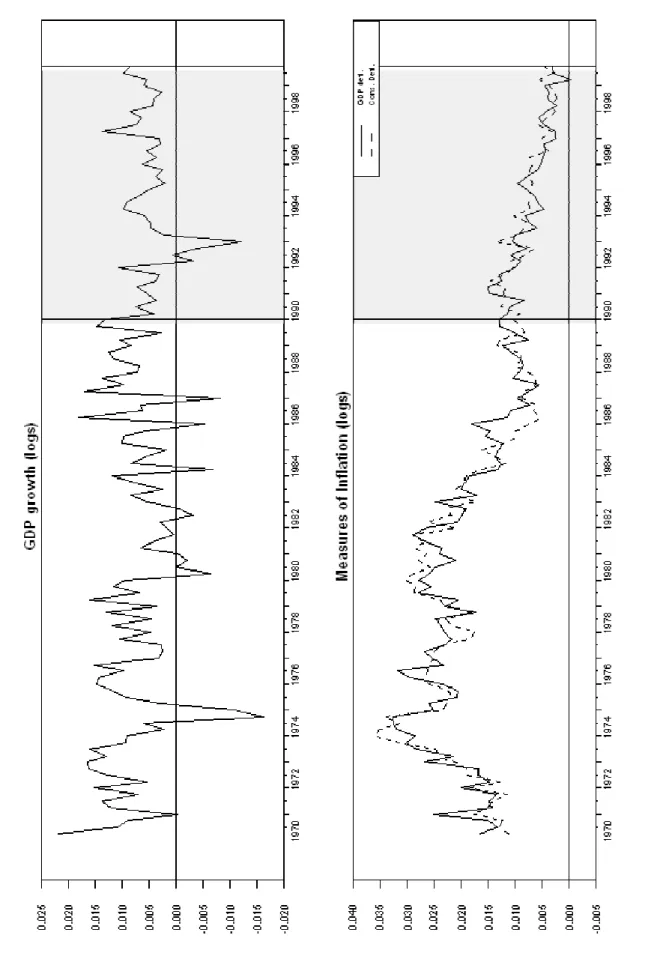
alternative to the AWM. Furthermore, they offer specific challenges in a forecasting exercise. As shown in Figure 1 (upper panel), GDP growth (in the form of first difference of log of real GDP) shows a low degree of persistence and a noticeable degree of variability. The lower panel of Figure 1 shows GDP deflator inflation and consumption deflator inflation, again in the form of first difference of log of each variable. Two outstanding facts in the figure regarding these two series is their evident higher persistence, on the one hand, and the likely presence of shifts in their underlying means, on the other. Furthermore, although both variables broadly co-move, short but conspicuous separations take place here and there.

This is as far as a simple exposition of the exercise can go, but there are obviously a large number of details that need be described for the reader to fully understand the whole exercise. These details can be presented under five general headings: how the recursive forecasts are performed; how exogenous variables are dealt with; how residuals are projected; how the model is re-estimated; and, finally, what are the alternative benchmark models. The next five sub-sections deal with these points.

3.1 The forecasting steps

The steps taken for the out-of-sample exercise were the following. For each model, a forecast for quarter-on-quarter change in the log of the variables was run starting in 1996Q1 with models (i.e., the AWM or the benchmark models) estimated using data until 1995Q4. Forecasts were run for the following eight quarters ahead and the corresponding forecast errors were collected. Thus, this forecast in particular generated one instance of 1-step-ahead to 8-step-ahead forecast errors. The models were then re-estimated using the sample until 1996Q1 and a new forecast starting in 1996Q2 was run for eight quarters, from which a new instance of 1-step-ahead to 8-step-ahead forecast errors were collected. The exercise was repeated for each quarter between 1996Q1 to 1999Q3, each time for 8 periods ahead or as many as the observations would allow. After the exercises were run, errors were collected according to the number of periods ahead to which they correspond. The final number of 1-step-ahead errors was thus 16, while the total number of 8-step-ahead errors was 9. For each of the 8 generated series of forecast errors the average mean, the standard deviation of the forecast error and the average RMSE were calculated and are reported in the tables described below.

The steps taken for the in-sample exercises were similar, with the exception that the re-estimation step was skipped: the AWM was used in its standard specification (broadly estimated until 1998Q4) and the benchmark models were used as estimated with their full sample. Rolling forecasts were started in 1990Q1 and were performed, as before, until 1999Q4. Taking advantage of the higher number of forecasts done, the longest forecast horizon was increased to 12 steps ahead, i.e. projections were run for 1- to 12-steps-ahead forecasts, generating from 40 1-step-ahead forecasts to 29 12-step-ahead forecasts.

Last but not least, both in-sample and out-of-sample forecasts were repeated with the updated dataset. Only the out-of-sample ones will be reported due to their higher relevance. The exercise was done for the European monetary union (EMU) period (1999Q1-2006Q4), using models estimated until 1998Q4 but not

re-estimated, in order to avoid forecast loses due to variability in parameters. 10

3.2 Treatment of additional exogenous information

One important issue arising was how to treat exogenous variables. Key exogenous variables that could affect the outcome comprise foreign variables (output, output prices and oil and commodity prices) and fiscal variables. As a first approximation, these were simply taken as observed. Another set of series that are

typically endogenous but (following central-bank forecasting convention) whose equations were dropped

were the exchange rate and the interest rate. The two equations describing the law of motion for these two variables were calibrated from well-known theoretical constructs, i.e. the UIP condition and a standard Taylor rule, and tend not to be seen as appropriate for a forecasting exercise. Put simply, there is no warranty that these rules are a reflection of relevant structural features in the data. These two variables were thus also kept at their observed values.

It may be argued that the use of exogenous AWM variables as observed may be problematic. As a robustness check, therefore a 7-variable VAR was estimated with the following series in levels: domestic output, domestic prices, foreign output, foreign output prices, oil and commodity prices, domestic interest rate, euro exchange rate. The VAR was estimated with and without a linear time trend, results for the former case being reported because of their higher interest. An SVAR version (using a Cholesky decomposition based on the causal ordering above) of the same was derived whose equations for foreign variables and the interest and exchange rates were then added to the AWM. Forecasts with both the AWM and the AWM

supplemented with equations from the SVAR were run for all the exercises reported. 11

3.3 Treatment of residuals

Among exogenous information needed by the model, one received a considerable amount of attention: the residuals of the estimated equations. As already stated, one of the crucial aspects of the exercise is to disentangle potential parameter instability from the presence of unaccounted-for structural breaks in assessing forecast failure. As already said, Hendry and Clements (1999) claim that “deterministic shifts” account for most systematic forecast failures, which they describe as un-forecastable breaks in equilibrium means. These breaks lead to large and persistent errors in forecasting precisely because they last for a long period, possibly forever. The fact that all the estimated equations in the AWM include a long-run component in the form of an equilibrium-correction mechanism can be exploited at this point: an intercept correction of these equations that is not subsequently reversed can be understood as reflecting a deterministic shift of this kind. Thus, how residuals are treated in these experiments is a crucial part of the exercise.

One way to assess the importance of this factor in the AWM is by testing different residual-projection

approaches and assessing their impact on forecast performance. In practice, what is done is projecting the residual of each equation using information available at the time of the forecast and a number of simple projection strategies. (Note that only stochastic equations in the model are shocked, identities are unaffected by the procedure.)

In our exercises, we have considered up to seven residual projection strategies, of which four core residual projection strategies were the preferred ones. These strategies appear plausible, mirror what forecasters tend to do in practice, and have meaningful interpretations. For completeness, we offer here the definition of the four although, in the interest of brevity, only results for two of the projection strategies will be fully discussed in the text. We formalize them as follows:

1. Flat Projection Method: for each forecast, residuals (ut) were projected according to their mean over a long period of time (1985Q1 to the period previous to the start of the forecast in the out-of-sample exercise, same starting date to end of out-of-sample in the in-out-of-sample exercise):

t

T

k

t

u

u

u

¦

,

1

,...,

This method was used in two different forms. In the out-of-sample exercise, the residual was

projected as its mean over the periods preceding the forecast. Thus, it was projected as a constant that varied slightly for each forecast, according to its initial date. In practice, residuals were not very different across forecasts, as model re-estimation did not lead to large variations in parameter

values. In the in-sample exercise, instead, the value was kept fixed across replications at full-sample

values, for the original dataset, or estimation-sample values for the new dataset.

2. Smoothed-Outlier Projection Method: for each forecast, residuals were projected at the average value observed in the last four quarters before the start of the forecast:

¦

The method tries to strike a balance between considering that all residuals are shifts in the deterministic part of the forecast and acknowledging that true outliers might be present. The way to do that is by taking a moving four-quarter average of past residuals and assuming that the resulting average is the new terminal level for the variable.

3. Outlier Projection Method: for each forecast, residuals were at their last-observed value, i.e. the period preceding the first forecast period:

k T k

u

u_{tk t}, 1,...,

This method is similar to the previous one, except for the extreme assumption that last period's equation residuals are always signalling the onset of a deterministic shift.

4. Smoothed-Trend Projection Method: for each forecast, residuals were projected according to their last-observed trend, defined as the average change over the four periods preceding the forecast.

¦

This method is even more extreme than previous ones since the trend in the deterministic component of each forecast is revised each time an exercise is run. In practice, this approach implies that the analyst suspects a major specification failure in the model.

Note that the version of the AWM including SVAR equations was run with residual shifting also applied to the latter equations.

Finally, note that a few other residual projection strategies were pursued in our exercises. For completeness, and for the interest of some readers, these are described and motivated in Annex 1.

3.4 Re-estimation procedure

In re-estimating the model it was important to use as little information as possible belonging to the period to be forecast. This was achieved by, among other things, restricting the number of parameters originally calibrated, as the calibration could be seen as reflecting prior information based on the knowledge of the full sample. Among parameters that were nevertheless taken at their original calibrated value, the capital-share parameter was the most important. Other calibrated parameters taken unchanged were those in the wage and price equations on price expectations and the ECM term in the wage equation. In addition, the NAIRU embodied in the model was left unchanged at its full-sample value. It is highly unlikely that those calibrated terms will significantly affect the outcome of the exercise, due to their limited variability over our short forecast horizon.

The equations were simplified by dropping dummy variables effective in or after 1995Q4, the first period

estimated.12 _{Another simplification was the harmonization of the end-of-sample for all the equations.}

Although original equations were estimated with varying ending points, depending on data availability at

12 _{An alternative is to alter the specification of the equations to re-introduce dummy variables after the period in which they become}

effective. The decision to keep equations unchanged over recursive re-estimations was taken to simplify the exercise. This means that outliers in the period are more disruptive than otherwise, thus possibly again biasing results against the AWM.

the time of the original estimation, in the present recursive exercises all equations were estimated until a common ending point, the last possible period before starting each forecast. Notwithstanding all these points, the equations were largely similar to those reported in Fagan et al. (2005), and relatively stable over the 4-year period used (see Annex 3).

The version of the AWM using SVAR equations applied the re-estimation procedure also to these equations.

For the in-sample exercises, the model was used as taken.

3.5 Alternative benchmark models

The AWM was tested against simpler alternative models: an AR(2) model of each variable, and an ARX(2) augmented with exogenous information (foreign GDP and prices, exchange rate and interest rate) taken at their observed values. Both benchmark models were for the first difference of the log of the variable to forecast, and included a constant and two lags of the endogenous variable. The second also included the short-term interest rate (in levels) and the first difference of the exchange rate, foreign GDP, GDP deflator and oil and commodity prices. These variables entered contemporaneously and lagged once and twice respectively. The ARX(2) models were used to assess the effect of taking foreign variables as given in the data, the way this is done with the AWM when no SVAR equations are added to the model.

Furthermore, the 7-variable VAR used to derive the SVAR equations for foreign variables described above was also used as a benchmark model.

4.

Results

For clarity, results will be presented first for the simulated out-of-sample exercise, then for the in-sample

exercise and finally for the revised dataset. The first two steps will be used to assess the importance of

add-factoring using the dataset on which the AWM was estimated. The third step more thoroughly analyses out-of-sample behaviour of all the models by running forecasts over the EMU period using models estimated with data previous to EMU. Results under each heading will be presented for consumption deflator inflation in the first instance and then for the other reported variables.

An important caveat is that no formal test of forecast comparison will be made in the text. This reflects the nature of the exercise: as is well known, out-of-sample tests for forecast comparison when models are nested have non-standard distributions. The procedure to test against the proper test sizes is to bootstrap the forecasts. Since the AWM can be deemed to nest all the alternative models contemplated, since there is an interest in analyzing multi-step forecasts, and since bootstrapping the AWM for the large number of tests considered is certainly computationally prohibitive, we follow a relatively more narrative approach.

4.1 Simulated out-of-sample exercise

4.1.1 Forecasts of consumption deflator inflation

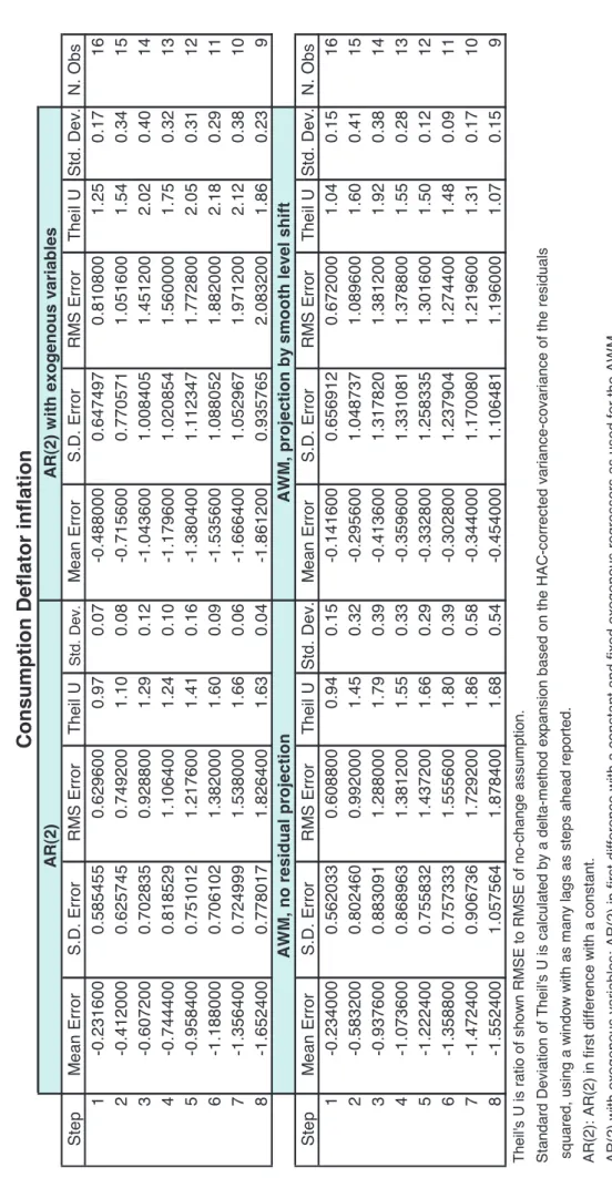
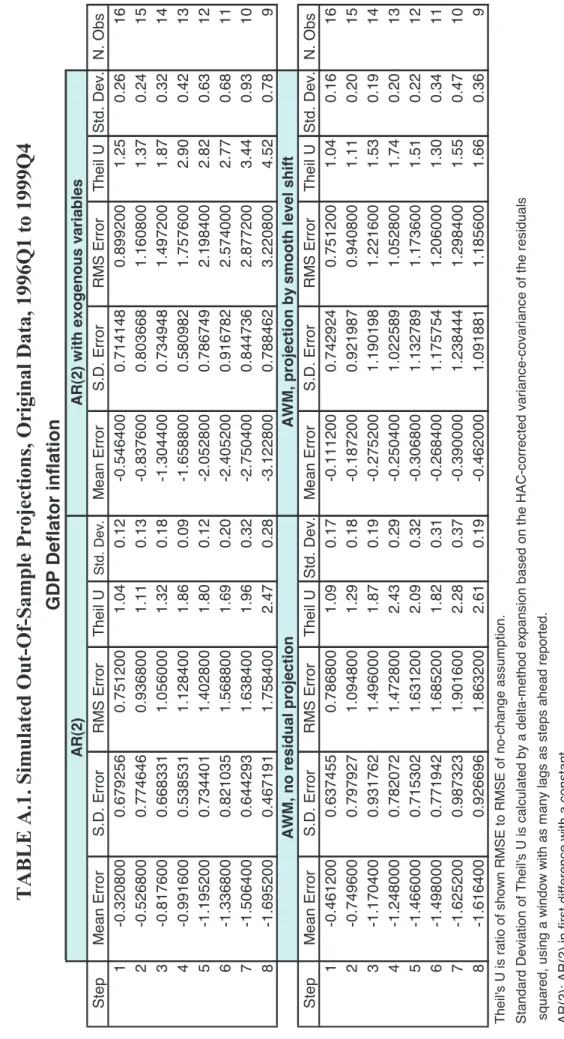
Table 1 shows the basic forecast statistics for the out-of-sample exercise for the consumption deflator quarter-on-quarter inflation. The table shows the mean error, the standard deviation (S.D.) of the forecast error, the RMSE and Theil's U statistic (together with its standard deviation) for exercises covering from 1- to 8-step ahead forecasts, run for the period 1996Q1 to 1999Q4. The mean error, the S.D. and the RMSE are reported as 400 times their estimated values, to ease their reading. Models for which results are reported are the AR(2) model, the ARX(2) model and the AWM.

[INSERT TABLE 1]

Results for the AWM are shown for the announced residual-projection strategies: no residual projection, and residuals as smooth level shifts. Theil's U statistic is the ratio between the corresponding RMSE and the RMSE resulting from a naïve forecast in which inflation is projected unchanged since it was last observed. Thus, a U statistic of less than one indicates that forecasts from the model under test is to be preferred to the naïve forecast. The standard deviation attached to each U statistic is the non-parametric estimate of the ratio of the two RMSE involved in its calculation.

A number of facts can be noticed:

None of the models clearly beats the no-change forecast at short horizons (h=1), after which all models

worsen substantially.

In terms of Theil's U statistic, the smoothed-outlier projection is clearly to be preferred to the other

models as h increases.

In terms of mean error (bias), the smoothed-outlier projection strategy is by far the better.

4.1.2 Forecasts for the other variables

It is worth pointing out to what extent these results apply to the other two variables analyzed, GDP deflator inflation and GDP growth. GDP deflator inflation is forecast with similar accuracy across models at short horizons, but not at long horizons, in which the smooth-outlier projection strategy offers the best results. Regarding forecast biases, the good performance of the AWM with smooth level shifts found with the consumption deflator inflation is also present in this case. The worst GDP growth forecasts at short and medium horizons, in terms of RMSE, are from the AWM. For longer horizons, the AR(2) is the best one and the ARX(2) the worst one, with the AWM closer to the former than to the latter. Contrary to what happens to inflation, the bias is not clearly affected by the use of add-factors: it actually increases slightly. In summary, one could argue that the AWM, although no worse than standard forecasting benchmark models, needs some help from exogenous level shifts, at least for inflation. The implications of this are that the model is not properly capturing stable long-run relationships. As will be shown, though, a deeper analysis of the RMSE leads to a partial reassessment of this conclusion. We will proceed to decompose the reported RMSE in order to show that although level shifts are important to counter model biases, their overall impact on forecast accuracy could be negative. Although deterministic shifts help reducing

first-moment discrepancies between model and the data-generation process (and this seems to be a robust finding), this happens at a cost in terms of second-order moments than at times more than balances their potential benefit.

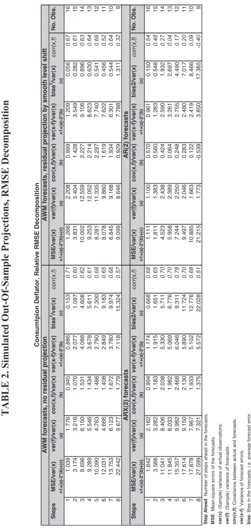
Table 2 shows the RMSE decomposition of the forecasts for the four models analyzed in Table 1. In the table, the decomposition in (12) is shown relative to the variance of the variable, in order to enhance the

readability of the table.13

[INSERT TABLE 2]

One striking feature in the table is the huge disparity in biases (squared) between the AWM with

smooth-outlier projection and the rest, at least for large h. This is the main mechanism explaining the good

behaviour of this use of the model for long-horizon forecasts. (The ARX(2) model is clearly worse on this account, though, which explains its very bad behaviour at medium to long horizons.) Finally, the relatively good performance of the AR(2) at short horizons is coming mostly from its low forecast variance. This is in contrast with the relatively low correlation between forecast and actual for this model. The low forecast variance means that AR(2)-based forecasts converge to a point faster than the other models, a feature which is not desirable per se. In a word, level shifts are adding to the AWM's forecast variance but this is balanced by a reduction in the forecast bias. Thus, level shifts seem to have a positive impact to the extent that they

get rid of bias faster than they add to forecast variability. 14

Unfortunately, no firm conclusions can be drawn from the exercise due to the small number of forecasts run, as is made clear by the large standard deviations of the U statistics. Furthermore, forecast variance depends to an unknown extent on parameter re-estimation, with more complex models bound to lose more on this account due to higher number of parameters. In a word, results in Table 2 may bias the picture against the AWM (or indeed any structural macro-model) simply because of its higher complexity. It is thus necessary to reassess results in the light of constant-parameter models.

4.2 In-sample exercise

4.2.1 Forecasts of consumption deflator inflation

As a first steps, results spanning 1996Q1 to 1999Q4 were assessed using the full-sample version of the models and lent weight to the view that model re-estimation adds significantly to the variance of the forecast without affecting much the bias. Hence, model re-estimation has in general a small beneficial impact on forecast bias, but adds to forecast variability to an extent that often more than balances this factor. The question is thus whether re-estimation is strictly necessary to test the model: according to Inoue and Kilian (2005) this is not so, as all relevant inference can be obtained in-sample. Based on the strength of their views and the evidence gathered so far in our analysis, it was decided to repeat the forecasts using the AWM in its final form, i.e. with parameters estimated using the full sample.

13 _{In other words, the raw numbers – which were very small – have been re-scaled by the variance of the observations used to}

calculate the corresponding RMSE. Please note that the column with the relative covariance, label 'cov(x,f)/var(x)', differs by construction from the correlation between actual and forecast. In order to ease interpretation of the table, a memo column with the correlation between the two has been included in each entry.

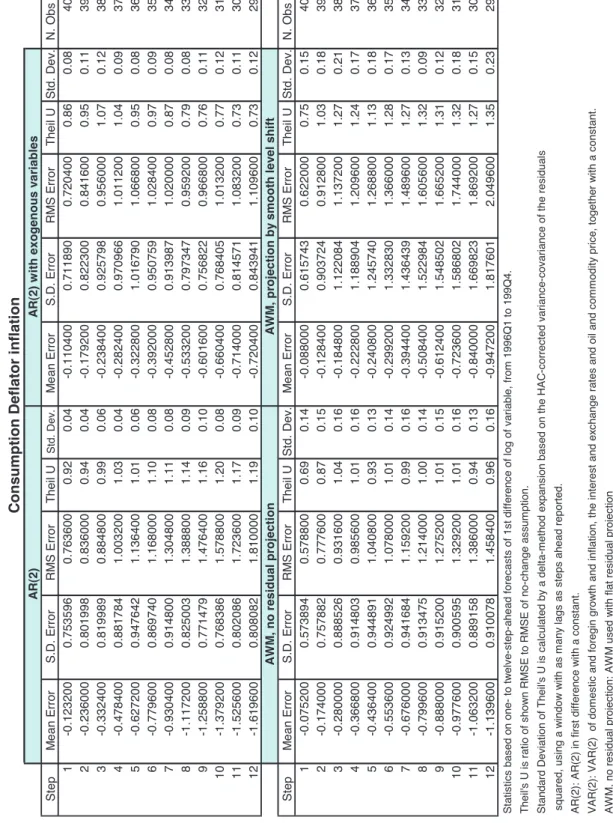
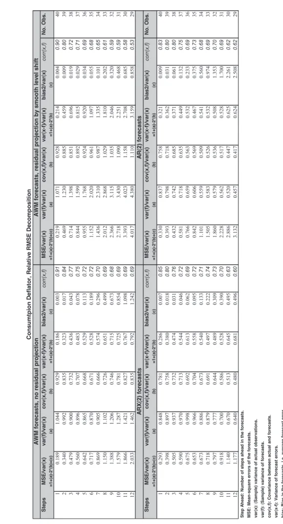
Table 3 presents results for a repetition of the exercise described in Table 1, but skipping the re-estimation step for all the models and with an extended period over which the exercise is run, i.e. 1990Q1 to 1999Q4. Table 4 presents the corresponding RMSE decomposition.

[INSERT TABLES 3 AND 4]

Results in Table 3 have been drawn from simulated in-sample forecasts (i.e., dynamic simulations) spanning the mentioned period, which means that as much as 40 forecasts were available. This has the merit of significantly reducing the variability seen in the numbers in tables 1 and 2 and considerably clarify the picture. Taking advantage of that, forecast horizon has been increased to allow for forecasts up to 12 periods ahead.

One of the main conclusions from tables 3 and 4 is that the AWM with no residual projection is now clearly better than projecting with the smooth level shift projection. As can be seen in Table 4, this stems basically from a lower variance of the forecast in the former case. Thus, although it is still the case that shifting the levels of the residuals leads to lower forecast bias, this is more than offset by forecast variability induced by shifting the levels. (In both cases the correlation between actual and forecasts is similar.) Comparing to the benchmark models, Table 3 shows that the ARX(2) model now performs better, but with the caveat that this seems to come mostly from much lower bias, implying that this model is seriously impaired by parameter re-estimation. The AR(2) model performs relatively worse than previously, at least in comparison with the no-residual projection, in particular due to higher bias.

4.2.2 Forecasts for the other variables

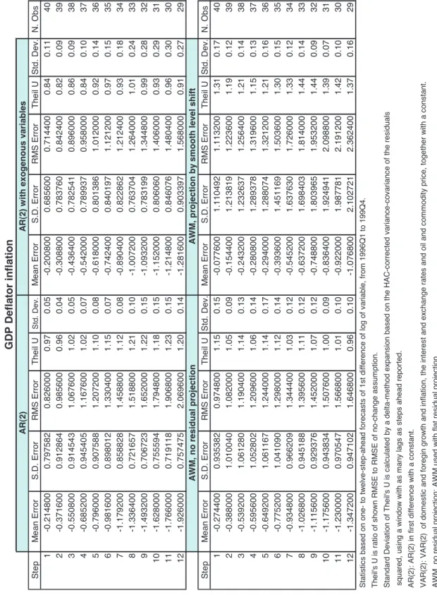
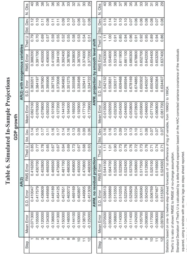
Finally, tables 5 and 6 present results for the other two variables of interest: GDP deflator inflation and GDP growth. Note that the mean error, the S.D. and the RMSE for GDP growth are multiplied by 100 (instead of 400, as for the inflation series).

[INSERT TABLE 5]

Table 5 for GDP deflator inflation clearly indicates that the AWM with no residual-projection strategy fares better than when residuals are projected with smooth level shifts, in particular at long horizons. Note, however, that biases are everywhere relatively large, sometimes as high as in the out-of-sample exercise. Compared to benchmark models, the AWM (with no residual projection) is consistently worse in short-term forecasts, but beats the AR(2) model and comes close to the ARX(2) for long-term forecasts.

Finally, Table 6 shows results for GDP growth. As was the case in the out-of-sample exercise, bias reduction from add-factoring is not clearly present. Otherwise, all models behave in a similar way, in special as regards long-term forecasts.

[INSERT TABLE 6]

In general, it is the case that the AWM without residual projection fares better than the smooth-level-shift approach, contrary to the out-of-sample findings.

Results using the VAR (with trend) beat the other models, including the AWM, in terms of RMSE for all the reported variables. Furthermore, biases were in all cases, except for GDP growth, smaller. Charts 2, 3

and 4 present the biases for the three variables and all the forecasts run using the original dataset. It may be noticed that the AWM with smooth-outlier projection is still the best, in terms of bias, for GDP growth. It

also closely tracks the VAR for short-horizon forecasts (h from 1 to 5 quarters ahead) for consumption

deflator inflation. For GDP deflator inflation, on the other hand, the VAR clearly beats all other models. It must be concluded that the VAR (the only model including an explicit trend) is clearly outstanding in terms of forecast bias for inflation. It is clearly the model to beat.

4.3 Forecasting in EMU

The last exercise involves the use of the most recent dataset spanning 1970Q1 to 2006Q4. As explained in section 3, the new data are very significantly changed from the older dataset over their entire span. In particular, the short-term dynamics of the series may have been affected, which in theory could bias results in favour of add-factoring. To assess the effects of add-factoring more thoroughly, the procedure has been applied in this section to all the models. Nevertheless, the previous in-sample results, which saw a positive impact on forecast bias but a negative impact on overall accuracy from residual projection, should be borne in mind when comparing results.

Forecasts will now focus on the EMU period, 1999Q1 to 2006Q4, for empirical- and policy-relevance reasons. The most revealing exercise involved EMU forecasts from models estimated until 1998Q4 which were not recursively re-estimated for the forecasts. Thus, the exercise was done out of sample but the RMSE of the forecasts was not affected by model estimation. Exercises were also run with recursive model re-estimation and full sample estimates (i.e., estimates going until 2006Q4) but will not be reported due to their

lower interest.15

4.3.1 Forecasts for inflation

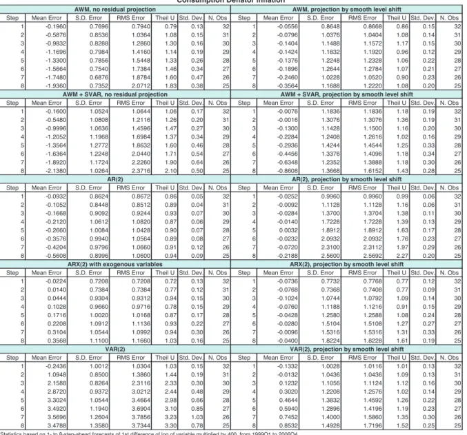
As far as results in this section are concerned, distinguishing between consumption deflator inflation and GDP deflator inflation is unnecessary. Both will be discussed under the same heading. The main findings are, in the first place, the worse performance of all models compared with the previous out-of-sample exercise; in the second place, the pervasiveness of bias reduction when add-factors are used; in the third place, the change in the ranking of models. All the results discussed below can be found on table 7.

[INSERT TABLE 7]

The first point is in all likelihood a reflection of the change in the behaviour of trend inflation across samples, discussed below, since models estimated in the first part of the sample are not suited to forecasts

the second part. The second point comes from the fact that bias 8 steps ahead has been reduced in each

single case. Furthermore, biases have often gone from being higher than forecast error variance to being much lower. Although, as said, the new dataset could bias results in favour of add-factors for the AWM , the point should not hold for the other models, whose dynamics are well adapted to the new dataset. The third point comes from the fact that the best model in the previous sections, the VAR model, is now among the

15 _{Results for recursive re-estimation of models and full-sample estimation of models are included in an annex to the working paper}

worst ones. Only subjecting the VAR to add-factor correction brings it back to the fore in terms of forecast performance.

The reading of the results should be relatively straightforward: for inflation, the evolution of the deterministic component of the underlying behaviour of the series matters (probably) more than the type of model used to produce the forecasts. Models that do not include explicit roles for trend changes, such as the AWM or the AR(2) model, tend to give consistent but lacklustre results over different samples, except if their residuals are suitably projected. Models that include explicit trends, such as the VAR, show extreme performance across samples, from exceptionally good to exceptionally bad, unless again their residuals are projected. Furthermore, the VAR is the only model consistently under-predicting inflation, as the other models mostly over-predict it. This would be the case if an underlying negative trend over the estimation period is gone in the forecast period.

It is unavoidable to conclude that the underlying deterministic or trended behaviour of inflation has significantly changed before and after EMU. Although monetary policy is the main suspect in both parts of the sample as to what caused this, proving this point is beyond the scope of this paper. Suffice to say that there is strong evidence that most estimated models used to forecast inflation are badly adapted for the EMU period. Instead, inflation forecasts should be performed with either models in which the deterministic component is modelled in sophisticated ways, or with models robust to changes in trends, independently of

how good or bad they fit the data over the estimation period.16

4.3.2 Forecasts for growth

As with inflation, add-factors reduce bias 8 steps ahead in all cases, sometimes dramatically. Contrary to inflation, though, the ranking of models in terms of their long-term ability to forecast is not seriously perturbed. The only general point of relevance is the negative bias in long-horizon forecasts across models, which would point to a slight decrease in trend GDP growth over the two samples. But certainly the previous strong evidence of a change in trend does not seem to be present.

4.4 Further exercises on inflation trends

Is the conclusion that inflation saw a change in trend over the sample borne out by further evidence? One

way to briefly check for this is to assess the extent to which models robust to changes in trend behave.17

Since this is best done with simple models, variations over the AR models used in the paper were used to assess the effects of including or excluding stochastic or deterministic trends in this basic simple model. In particular, the basic AR(2) model was changed and re-estimated, always until 1998Q4, and used to produce forecasts of consumption deflator inflation for the period 1999Q1 to 2006Q4 with the following alternative specifications:

2nd difference of the consumption deflator (in logs), with two types of deterministic components: none,

and a constant;

16 _{The obvious alternative is to wait sufficiently long to have long time series covering the EMU period.}

1st _{difference of the same variable (i.e., its inflation rate), with three types of deterministic components:}

none, a constant, and a constant and a trend.18

Lags in the equations were selected using classical LR tests, resulting in 1 lag for the 2nd_{-difference models}

and 2 lags for the 1st_{-difference ones. A summary of the models, including their roots, can be found in table}

8. All the estimations are consistent in that at least one unit root is present (as one root is always either imposed at 1 or close to 1), one further large root is present (close to one when estimated unless a trend is included) and a smaller root is present (at around -0.3). The equations were used to produce forecasts of inflation (quarter-on-quarter, as in the rest of the paper), by suitable accumulation of the raw forecasts in the

case of the 2nd_{-difference equations.}

[INSERT TABLE 8]

Note that the 1st_{-difference equation with constant and trend and the 2}nd_{-difference equation with constant}

should import the trend into the forecast period, leading to undershoots (positive bias), and that the 1st

-difference equation with constant should import the sample mean of inflation into the forecast period,

leading to overshoots (negative bias). The 2nd-difference equation with no deterministic component does not

have a terminal condition for the inflation rate and is our principal candidate for robust forecast model. Last

but not least, the 1st_{-difference model with no deterministic component implies a terminal null inflation rate}

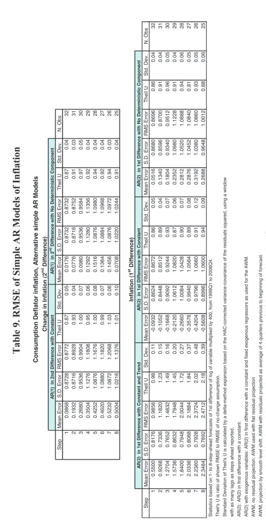
and is thus inconsistent with any meaningful DGP of the data, but is included because its quasi-unit root, probably spurious, turns this equation into basically a replicate of the previous one. Results are reported in table 9.

[INSERT TABLE 9]

From table 9, it is clear that most of the prior views above have been validated. Furthermore, the two models

identified as more robust to changes in trend turn out to be the best ones: the 2nd_{- and 1}st_{-difference models}

with no deterministic component. The 1st_{-difference model with constant comes a close second, while the}

1st_{-difference model with constant and trend is clearly the worst one, with the large terminal bias (at three}

times the standard deviation of the forecast error) explaining most of the outcome. Note that this last model is the preferred one in sample.

5.

Conclusions

We examined the performance of different residual projection strategies on forecast performance, using a large macro model of the euro area and smaller time-series-based models. The macro model, the AWM, is actively used for forecasting and policy simulation purposes. In our exercises, we attempted to outline a careful and comprehensive methodology; in effect, laying out a road map for how other macro-model users may evaluate residual projection strategies in their own environment.

Aspects of forecast failure identified in the academic literature (but typically employed with “small” systems) were applied. A number of tests were carried out trying to assess the relative predictive

18 _{Note that including a trend in the 2}nd_{-difference model was unnecessary, as the 2}nd _{difference of the consumption deflator is}