Forecasting euro area inflation:
Does aggregating forecasts by HICP component
improve forecast accuracy?
1Kirstin Hubrich2
Research Department, European Central Bank April, 2004
Abstract
Monitoring and forecasting price developments in the euro area is es-sential in light of the two-pillar framework of the ECB’s monetary pol-icy strategy. This study analyses whether the accuracy of forecasts of aggregate euro area inflation can be improved by aggregating forecasts of subindices of the Harmonized Index of Consumer Prices (HICP) as opposed to forecasting the aggregate HICP directly. The analysis includes univariate and multivariate linear time series models and dis-tinguishes between different forecast horizons, HICP components and inflation measures. Various model selection procedures are employed to select models for the aggregate and the disaggregate components. The results indicate that aggregating forecasts by component does not necessarily help forecast year-on-year inflation twelve months ahead.
JEL Codes: E31, E37, C53, C32
Keywords: euro area inflation, HICP subindex forecast aggregation, linear time series models
1A first version of the paper was drafted while the author was researcher at the Dutch
Central Bank. I thank Lutz Kilian and Peter Vlaar for helpful discussions. I also thank Filippo Altissimo, G¨unter Coenen, Peter van Els, Neil Ericsson, Gonzalo Camba-M`endez, Michael Clements, Jan Groen, David Hendry, Tohmas Karlsson, Hans-Martin Krolzig, Helmut L¨utkepohl, Massimiliano Marcellino, Jim Stock, Harald Uhlig and two anonymous referees as well as participants of the European Econometric Society Meeting (ESEM) 2002 in Venice, a conference at the Banque de France, the annual conference of the German Economic Association 2003, theEC2Conference 2003 in London and seminar participants
at the Dutch Central Bank, the Working Group of Econometric Modelling of the ESCB, CentER/Tilburg University, the Tinbergen Institute, Amsterdam, and the University of Oxford for useful comments. The usual disclaimer applies. The views expressed in this paper are those of the author and do not necessarily reflect those of the European Central Bank.
2European Central Bank, Research Department, Kaiserstrasse 29, D-60311 Frankfurt
1
Introduction
The primary objective of the ECB’s monetary policy is price stability. Price stability has been defined by the Governing Council of the ECB, according to the clarification in May 2003, as a year-on-year increase in the Harmonized Index of Consumer Prices (HICP) for the euro area of below, but ”close to 2% over the medium term” (European Central Bank, 2003b).
The European System of Central Banks (ESCB) is monitoring and pro-jecting prices under the two-pillar approach of the ECB’s monetary policy strategy to assess price developments in the euro area. Since December 2000 the ECB has been publishing its inflation projection for the euro area.3
Fur-ther insights regarding the performance of different forecasting strategies for euro area inflation are highly relevant for policy makers and ECB observers. In the context of forecasting euro area inflation the question arises to what extent the forecasting accuracy of different time series models for ag-gregate inflation can be improved by modelling subcomponents of inflation and aggregating forecasts based on these models. Contemporaneous aggre-gation of forecasts may be considered in two dimensions: the aggreaggre-gation of national HICP forecasts for euro area countries and the aggregation of HICP subcomponent forecasts for the euro area.
The forecasting accuracy of aggregating country-specific forecasts in com-parison with forecasts based on aggregated euro area wide data has been analysed on the basis of a broad range of models in Marcellino, Stock & Watson (2003). Other studies have focused on specific methods of incorpo-rating national information into forecasts of euro area wide inflation. For example, Angelini, Henry & Mestre (2001) and Cristadoro, Forni, Reichlin & Veronese (2001) employ dynamic factor models in this context.
In contrast to these studies, the aim of this analysis is to compare the accuracy of methods of forecasting aggregate HICP directly as opposed to aggregating forecasts for HICP subcomponents. The analysis presented is based on data for the euro area as a whole as these are the data rele-vant for the monetary policy of the ECB. Another study that has investi-gated aggregation across HICP subcomponents is Espasa, Senra & Albacete (2002). That study is restricted to ARIMA models and to vector error correction models (VECM) that impose cointegration relations between the HICP subindices. In contrast, in the present study a broad range of models and model selection procedures is employed, that include macroeconomic predictors for inflation. The set of methods employed in this study is dis-cussed below. Differences between the results in Espasa et al. (2002) and those presented in the current study arise due to different methods employed
3The word ’projection’ in contrast to forecasting is used by the ECB to indicate that
the published projections are based on a set of underlying technical assumptions, including the assumption of unchanged short-term interest rate. In contrast, no assumptions for the development of any of the variables over the forecast horizon are made in this study.
as well as the different transformation of HICP underlying the evaluation of the relative forecast accuracy, i.e. here I consider year-on-year inflation forecasts relevant from a monetary policy perspective instead of month-on-month inflation forecasts. Furthermore, a longer forecast horizon of up to 12 months as well as a longer sample and forecast evaluation period are employed here.
The debate about aggregation versus disaggregation in economic mod-elling goes back to Theil (1954) and Grunfeld & Griliches (1960). One strand of that literature has focussed on the effect of contemporaneous aggregation on forecast accuracy. There are two main arguments for aggregating fore-casts of disaggregated variables instead of forecasting the aggregate variable of interest directly. One rationale is that by disaggregating the individual dynamic properties can better be taken into account and, therefore, the disaggregate variables can be predicted more accurately than the aggregate variable. Modelling disaggregated variables may involve using a larger and more heterogenous information set, and specifications may vary across the disaggregate variables (see Barker & Pesaran, 1990b). A second argument in favour of disaggregation is that forecast errors of disaggregated components might cancel partly, leading to more accurate predictions of the aggregate (also see Clements & Hendry (2002) for a discussion on forecast combination as bias correction).
In contrast, it may be argued that to forecast the aggregate directly is the superior strategy. For example, the models for the disaggregate vari-ables will in practice not be correctly specified (see Grunfeld & Griliches, 1960). A misspecified disaggregate model might not improve the forecast accuracy for the aggregate, especially in the presence of shocks to some of the disaggregate variables, as will be seen in the analysis presented in this study. On the other hand, a well specified model does not necessarily imply higher forecast accuracy either. An additional argument against disaggrega-tion for forecasting the aggregate is that unexpected shocks might affect the forecast errors of some of the disaggregate variables in the same direction so that forecast errors do not cancel.
In this study, I examine whether aggregating inflation forecasts based on HICP subindices is really better than forecasting aggregate HICP inflation directly. I analyse the role of a number of factors that based on asymptotic theory and Monte Carlo simulations have been found in the literature to affect the role of disaggregation on forecasting accuracy. They include i) different forecast models, ii) different model selection procedures, iii) differ-ent forecast horizons, and iv) differdiffer-ent inflation measures (e.g. aggregate ’headline’ inflation including all subindices versus HICP inflation excluding unprocessed food and energy prices, sometimes referred to as ’core’ infla-tion).
The forecasting methods include a random walk model, a univariate au-toregressive model and vector auau-toregressive models based on various model
selection strategies. Univariate and multivariate linear time series models are chosen for the comparison since these are often used for forecasting infla-tion in Europe on a nainfla-tional or euro area wide level. Vector error correcinfla-tion models have not been included in the comparison since those models may fail badly in forecasting in the presence of structural breaks in the equilib-rium mean (see e.g. Hendry & Clements (2003)).4 Non-linear time series
models are not considered in the current paper due to the short time series available for estimation.5 Time-varying parameter models are not
consid-ered here, either. Stock & Watson (1996) suggest that gains from using time varying parameter models for forecasting are generally small or non-existent, especially for short horizons.6
Various model selection strategies are employed in this study to select models for the aggregate HICP and its disaggregate components. These include choosing an information set guided by economic theory where the same model specification is chosen for each of the subcomponents. The model selection procedures also include the Schwarz information criterion (SIC) (Inoue & Kilian, 2003) as well as a general-to-specific modelling strat-egy implemented in the software package PcGets (Hendry & Krolzig, 2001).7
The latter model selection procedures allow for varying specifications across subcomponents in terms of lag order and / or variables included.
The remainder of the paper is structured as follows: In section 2 some asymptotic and small sample simulation results from the literature regard-ing the relative forecastregard-ing performance of aggregated forecasts of time series subcomponents are discussed. Section 3 presents the data used in the anal-ysis. The forecast methods and model selection procedures on which the forecast method comparison is based are outlined in section 4. In section 5 the empirical results for the relative forecast accuracy of the aggregated versus the disaggregated approach to forecasting euro area inflation are pre-sented and discussed. Finally, in section 6 I draw some conclusions.
4Espasa et al. (2002) employ a VECM to forecast aggregate euro area inflation taking
into account cointegration between HICP subindices and find that in this case disaggre-gation improves forecast accuracy 9 months ahead for monthly inflation.
5An exposition of the forecasting performance of non-linear models can, for example,
be found in Clements & Hendry (1999, Ch.10). See also Marcellino (2004) for some promising results using non-linear models for longer euro area macroeconomic series that are extended backwards by aggregating available country data.
6See Canova (2002) for a recent more favourable evaluation of the forecasting
perfor-mance of Bayesian time varying parameter models, whereas his results for BVARs are less favourable.
7For an analysis of the role of model selection strategies on forecasting failure, see e.g.
2
Forecasting contemporaneously aggregated time
series: Some results from the literature
In empirical analysis the researcher often has to work with temporally or contemporaneously aggregated variables. Recently, there has been renewed interest in the consequences of temporal aggregation for empirical analy-sis (see e.g. Marcellino (1999)). Similarly, the effects of contemporaneous aggregation across national variables in the context of modelling euro area developments have received increasing interest.8 The focus of this study
is on analysing the effects of contemporaneous aggregation of subcompo-nents of time series variables on forecasting accuracy which in the empirical literature has received rather limited attention.9
Consider forecasting a contemporaneously aggregated variable that is defined as a variable consisting of the sum or the weighted sum of a number of different disaggregated subcomponents at time t. The contemporaneous aggregate can be written as
yaggt =w1yt1+w2y2t +...+wnytn, t= 1, ..., T,
where ytj (j = 1, ..., n) are the subcomponents of ytagg, n is the number of subcomponents considered andwj,j= 1, ..., n,are the aggregation weights. It is assumed that the aggregation weights are fixed, i.e. they do not change over time, and that wj > 0 and Pwj = 1. Thus, ytagg is assumed to be a
linear transformation of the stochastic processesytj. Two different forecasts of the aggregate will be considered in this study. The direct forecast of the aggregated variable, denoted as ˆytagg, and an indirect forecast of the aggregated variables by aggregating thensubcomponents forecasts ˆytj (j= 1, ..., n), i.e. ˆysub,tagg =Pwjyˆjt.
The issue of contemporaneous aggregation of economic variables has al-ready been discussed and analysed in an early contribution by Theil (1954) who argues that a disaggregated modelling approach improves the model specification of the aggregate. Grunfeld & Griliches (1960), however, point out that if the micro equations are not assumed to be perfectly specified, aggregation is not necessarily bad since the ’specification error’ might be higher than the ’aggregation error’.
Subsequent developments in the theoretical literature on the contem-poraneous aggregation of time series has focused on several themes. One strand has concentrated on deriving the nature of the data generating pro-cess (DGP) of the aggregated propro-cess if the subcomponents are assumed
8In addition to the papers on forecasting inflation in the euro area mentioned in the
introduction, e.g. Zellner & Tobias (2000) study the role of disaggregation in forecasting industrialized countries’ median GDP growth.
9One example is Fair & Shiller (1990) who consider disaggregated components for
to follow a certain DGP (e.g. Rose (1977) for ARIMA processes, Lippi & Forni (1990) for ARMAX models and Nijman & Sentana (1996) for GARCH models). Another strand of this literature has focussed on the effect of con-temporaneous aggregation on forecasting accuracy, for example Rose (1977), Tiao & Guttman (1980), Wei & Abraham (1981), Kohn (1982), L¨utkepohl (1984a, b,1987), Pesaran, Pierse & Kumar (1989), Van Garderen, Lee & Pesaran (2000). Leamer (1990) derives an optimal degree of disaggregation in terms of the prediction error.10
The main asymptotic and small sample simulation results that are of in-terest here are the following. If the DGPs of the individual subcomponents are known in terms of structure and coefficients, aggregating subcomponent forecasts is better in terms of a mean square forecast error (MSFE) crite-rion than forecasting the aggregate directly, MSFE(ˆysubagg) < MSFE(ˆyagg).
This result is due to the larger information set underlying the aggregated subcomponent forecasts. However, the usefulness of this result is limited because in practice the DGP is usually not known. If the assumption of a known DGP is relaxed and it is assumed that the unknown process order is estimated using a consistent order selection criterion, the relative forecast accuracy of the direct or indirect approach to forecasting the aggregate will depend on the true DGP.11 Under certain assumptions about the DGP12,
the aggregation of forecasts of the components can actually be inferior to forecasting the aggregated time series directly, MSFE(ˆyaggsub)>MSFE(ˆyagg).
The higher estimation variability of estimating the disaggregated processes instead of the aggregate process may increase the MSFE, in some cases even in large samples (L¨utkepohl, 1987, p.310). The relative forecast accuracy depends on the extent to which the systematic differences in the MSFE are offset by the effects of estimation variability.
Despite the effort to understand the theoretical aspects of the effect of disaggregation on forecasting, this line of research has yielded few practically useful insights. L¨utkepohl (1984a, 1987) presents Monte Carlo simulations to analyse the relative small sample accuracy in terms of the MSFE of directly forecasting the aggregate and aggregating subcomponent forecasts. He also includes modelling approaches where parsimonious specification is limiting estimation variability due to reduced precision of the estimates in short samples. The small sample simulations largely confirm the asymptotic
10Some related issues and results are presented in a paper by Granger & Morris (1976).
Granger (1990) provides a survey on aggregation of time series variables. Further papers, including a number of empirical studies, can be found in Barker & Pesaran (1990a).
11In case of a finite order DGP the asymptotic MSFE matrices are the same as in the
case of known process orders. In the case of an infinite order DGP an approximation of the MSFE can be derived asymptotically under the assumption that the AR orders of the processes fitted to the data approach infinity with the sample size (L¨utkepohl, 1987, p.73).
12I.e. if the true DGP does not have a representation with finite lag order and a finite
results. He finds that the small sample rankings of the two approaches are mixed and depend on the DGP. The results suggest that it is not necessarily better to aggregate the subcomponent forecasts instead of forecasting the aggregate. If the subcomponents are uncorrelated and the forecast horizon is short, then aggregating the subcomponent forecasts may lead to a lower MSFE for certain DGPs.
Overall, results from asymptotic theory and small sample simulations do not give a clear answer regarding the relative forecast accuracy of the disag-gregate versus the agdisag-gregate forecasting approach. Whether aggregation of subcomponent forecasts improves forecast accuracy is largely an empirical question. Therefore, an empirical out-of-sample forecasting experiment is carried out in this study. The aim is to gather insights about the effect of contemporaneous aggregation on forecasting accuracy for euro area HICP inflation at the center of interest of the ECB’s monetary policy.
I pay special attention to the potential role of macroeconomic predic-tors for HICP inflation. I allow for additional macroeconomic variables in a VAR framework and in this framework also consider different forecast horizons. In so doing, I employ different model selection procedures. In contrast, most of the asymptotic results regarding (dis-)aggregation in fore-casting either assume the true DGP to be known or correctly specified, or the model choice to be based on a consistent model selection criterion. In practice, estimation variability will be a main factor in reducing the relative forecast efficiency of models with a high number of parameters. Therefore, the model selection procedure is important in deriving the final model. One possibility is to employ information criteria to select the lag length of (V)AR models. L¨utkepohl (1984a) presents results for subset VARs where informa-tion criteria are also used to decide on deleting individual elements from the coefficient matrices. This model selection procedure leads to lower estima-tion variability due to parsimonious specificaestima-tion (also see Inoue & Kilian, 2003). Another possible way of choosing a parsimoniously specified model is to use the automatic general-to-specific model selection procedure of Hendry & Krolzig (2003) implemented in PcGets (Hendry & Krolzig, 2001). This model selection procedure has been included in the comparison presented below.
3
HICP aggregate data and subcomponents
The data employed in this study include aggregated overall HICP for the euro area as well as its breakdown into five subcomponents: unprocessed food, processed food, industrial goods, energy and services prices.
This particular breakdown into subcomponents has been chosen in ac-cordance with the data published in the ECB Monthly Bulletin and since the analysis of price developments of HICP subcomponents regularly presented
in the ECB Monthly Bulletin (see European Central Bank (2000, p.28)) is based on this breakdown. A range of explanatory variables for inflation is also considered.
The data employed are of monthly frequency13, starting in 1992(1) until
2001(12), i.e. T = 120 observations. This relatively short sample is deter-mined by the availability of data for the euro area and has to be split for the out-of-sample forecast experiment. A recursive simulated out-of-sample forecast experiment is carried out, where the first recursive estimation pe-riod starts in 1992(1) up to 1998(1), extending the sample by one month sequentially. The longest recursive estimation sample ends in 2000(12). This set-up allows for 36 forecast evaluation periods for the 1 to 12 step ahead forecasts (for more details, see section 5). Seasonally adjusted data have been chosen14because of the changing seasonal pattern in some of the HICP
subcomponents for some countries due to a measurement change.15,16 The
notation for the HICP subindices will be the following: HICP unprocessed food will be denoted puf, HICP processed food ppf, HICP industrial
pro-ductionpi, HICP energy pe and HICP services ps. Furthermore, aggregate
HICP will be denotedpagg.
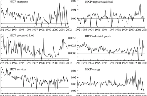
The aggregate HICP price index and the HICP subindices in logarithm are presented in Figure 1, whereas the month-on-month inflation rates (in decimals) and the year-on-year inflation rates (in %) of the indices are dis-played in Figure 2 and 3, respectively. Aggregate HICP, HICP processed food, HICP industrial production and HICP services in levels display a rela-tively smooth upward trend. In contrast, HICP unprocessed food and HICP energy exhibit a much more erratic development (see Figure 1). The annual inflation rates (see Figure 3) exhibit a downward trend for aggregate HICP, processed food prices, prices of industrial goods and service prices roughly until 1999. Unprocessed food and energy prices do not show a downward trend over the sample, but a sharp increase in 1999 due to oil price increases and animal diseases.
Diebold & Kilian (2000) show for univariate models that testing for a unit root is useful for selecting forecasting models. I have carried out Augmented Dickey Fuller (ADF) tests for all HICP (sub-)indices (in logarithm). The tests are based on the sample from 1992(1) to 2000(12), i.e. the longest of the recursively estimated samples. The tests do not reject non-stationarity for the levels of all (sub-)indices over the whole period.17 Non-stationarity
13Except for unit labour costs which are of quarterly frequency and have been
interpo-lated.
14Except for interest rates, producer prices and HICP energy that do not exhibit a
seasonal pattern.
15The data used in this study are taken from the ECB and Eurostat.
16The sensitivity of the results to using seasonally unadjusted data has been analysed on
the basis of a shorter sample. The results show no substantial change in the conclusions.
17The ADF test specification includes a constant and a linear trend for the levels and
1992 1993 1994 1995 1996 1997 1998 1999 2000 2001 2002 90 95 100 105 110 HICP aggregate 1992 1993 1994 1995 1996 1997 1998 1999 2000 2001 2002 95 100 105 110
115 HICP unprocessed food
1992 1993 1994 1995 1996 1997 1998 1999 2000 2001 2002
90 95 100 105
110 HICP processed food
1992 1993 1994 1995 1996 1997 1998 1999 2000 2001 2002
95 100 105
HICP industrial goods
1992 1993 1994 1995 1996 1997 1998 1999 2000 2001 2002 90 100 110 HICP services 1992 1993 1994 1995 1996 1997 1998 1999 2000 2001 2002 100 110 120 HICP energy
Figure 1: HICP aggregate and subindices (in logarithms)
1992 1993 1994 1995 1996 1997 1998 1999 2000 2001 2002 0.000 0.002 0.004 0.006 HICP aggregate 1992 1993 1994 1995 1996 1997 1998 1999 2000 2001 2002 0.00 0.01
0.02 HICP unprocessed food
1992 1993 1994 1995 1996 1997 1998 1999 2000 2001 2002 0.000 0.001 0.002 0.003 0.004
0.005 HICP processed food
1992 1993 1994 1995 1996 1997 1998 1999 2000 2001 2002 0.0000
0.0025
0.0050 HICP industrial goods
1992 1993 1994 1995 1996 1997 1998 1999 2000 2001 2002 0.000 0.002 0.004 0.006 HICP services 1992 1993 1994 1995 1996 1997 1998 1999 2000 2001 2002 −0.02 0.00 0.02 0.04 HICP energy
1992 1993 1994 1995 1996 1997 1998 1999 2000 2001 2002 1 2 3 HICP aggregate 1992 1993 1994 1995 1996 1997 1998 1999 2000 2001 2002 0.0 2.5 5.0 7.5
10.0 HICP unprocessed food
1992 1993 1994 1995 1996 1997 1998 1999 2000 2001 2002
1 2 3
4 HICP processed food
1992 1993 1994 1995 1996 1997 1998 1999 2000 2001 2002
1 2
3 HICP industrial goods
1992 1993 1994 1995 1996 1997 1998 1999 2000 2001 2002 2 3 4 5 HICP services 1992 1993 1994 1995 1996 1997 1998 1999 2000 2001 2002 −5 0 5 10 15 HICP energy
Figure 3: Year-on-year HICP inflation (in %), aggregate and subindices
is rejected for the first differences of all series except the aggregate HICP and HICP services. For the first differences of the latter two series, however, non-stationarity is rejected for all shorter recursive estimation samples up to 2000(8) and 2000(7), respectively. Therefore and because of the low power of the ADF test HICP (sub-)indices are assumed to be integrated of order one in the analysis and modelled accordingly.
Further variables that enter the large VAR model in the forecast ac-curacy comparison are industrial production, y, and nominal money M3, m, producer prices, pprod, import prices (extra euro area), pim,
unemploy-ment,u, unit labour costs,ucl, commodity prices (excluding energy) in euro, pcom, oil prices in euro,poil, the nominal effective exchange rate of the euro,
N EER18, as well as a short-term and a long-term nominal interest rate,
is and il. This choice of variables for the multivariate model strikes a
bal-ance between including relatively few variables due to the short data series available for the euro area, and including the key variables that influence in-flation according to economic theory. All variables except the interest rates are in logarithms.19
lag on a 5% significance level.
18ECB effective exchange rate core group of currencies against euro.
19A reliable measure of administered prices and indirect taxes to be included in the
4
Forecast Methods and Model Selection
Six different forecasting methods using different model selection procedures are employed for both direct and indirect forecast methods, i.e. forecasting HICP inflation directly versus aggregating subcomponent forecasts. In case of the first three forecasting models the specification is the same across HICP subcomponents. The random walk with drift (RW) for prices has been in-cluded in the comparison. Furthermore, a simple Phillips curve model, as e.g. in Stock & Watson (1999), is employed including inflation and the change in unemployment in the VAR with 12 lags. This model will be de-noted V ARP h(12). The third model is a large VAR with 12 endogenous
domestic and international variables described in the data section above, allowing for 2 lags only due to the short sample (V ARInt(2)). The fourth
and fifth models are chosen based on in-sample information. A univariate autoregressive (AR) model is included in the comparison where the lag or-der is parsimoniously chosen using the Schwarz criterion, denoted ARSC.
Therefore, the lag order varies across the different components. A general-to-specific model selection strategy is employed to choose a VAR (V ARIntGets), implemented in the computer package PcGets by Hendry & Krolzig (2001), where the choice of variables and lag length is based on mis-specification tests, structural break tests, t- and F-block tests, encompassing tests and information criteria. A ’liberal’ selection strategy has been chosen implying a higher probability of retaining relevant variables at the risk of retaining ir-relevant ones. Since PcGets is in principle a single-equation procedure, a LR test has been carried out to test the null hypothesis that the specific models selected by PcGets for each of the variables included in the VAR are a valid reduction of the unrestricted reduced form VAR. This test does not reject for the models employed in the analysis. The model is selected by PcGets starting with a VAR including the large potential number of domestic and in-ternational variables as included inV ARint(2). In contrast toV ARint(2), for
this model type different variables and lag lengths are possibly chosen across different HICP subcomponents and the aggregate. The two methodsARSC
andV ARInt
Gets are included to analyse whether different specifications across
subcomponents in terms of lags and variables help to improve the forecast-ing accuracy of aggregatforecast-ing subcomponent forecasts. The automated model selection procedure implemented in PcGets is particularly useful in this in-vestigation since economic theory does not provide much guidance on how to model the disaggregate components of HICP. It should be noted, how-ever, that the general-to-specific model selection procedure implemented in PcGets does not aim at improving forecast performance, but is based purely on in-sample information.20 The sixth model employed is a VAR including 20The relation between model (mis-)specification and forecast accuracy has been
dis-cussed extensively in e.g. Clements & Hendry (1999, Ch3/4, 2001); see also Hendry & Clements (2003).
the five HICP subcomponents as endogenous variables, denoted V ARsubc.
The resulting subcomponent forecasts are then aggregated. This model is included to investigate whether taking into account possible correlations be-tween the subcomponents improves the (indirect) forecast of the aggregate. A lag length of two for theV ARsubc has been selected parsimoniously using
the SIC.
For all models, except for V ARInt
Gets and V ARsubc for which PcGets and
PcGive are employed, the forecasting exercise is carried out using GAUSS. All models are re-estimated for each of the recursive samples. Regarding the model selection procedures, the ARSC is applied for each of the recursive
samples. The lag lengths for the different component models and the aggre-gate model do hardly change over the different recursive samples, however. The PcGets procedure is applied to the shortest of the recursive samples until 1998(1).21
5
Simulated out-of-sample forecast comparison
To evaluate the relative forecast accuracy of forecasting aggregate HICP directly versus aggregating the forecasts of HICP subcomponents, a simu-lated out-of-sample forecast experiment is carried out. One to twelve step ahead forecasts are performed based on different linear time series models estimated on recursive samples. The main criterion for the comparison of the forecasts employed in this study, as in a large part of the literature on forecasting, is the root mean square forecast error (RMSFE).
The out-of-sample forecasting experiment
The forecasts produced by the respective method have to be transformed, since the forecast accuracy is to be evaluated in terms of root mean square forecast error (RMSFE) of year-on-year inflation. Note that the multi-horizon MSFEs do not allow forecast comparison between different represen-tations of the same system. Furthermore, switching the basis of comparison can lead to a change in ranking of the methods in this case.22 Therefore, it
is important to note that here the focus is on the comparison of all HICP (sub-)indices in terms of their forecast accuracy for year-on-year inflation rates since those are most relevant from a monetary policy perspective.
The aggregate HICP is a weighted chain index, where the weights change each year. Since the end of all recursive estimation samples is in 1998, 1999 and 2000, respectively, the aggregation of the forecasts is carried out using the HICP subcomponent weights of the respective end year of the estimation
21PcGets has also been applied to choose a new model for each recursive sample in the
context of forecasting total euro area HICP inflation. This did not improve the relative performance in comparison with the other methods.
period (at prices of December the previous year) which would be known to the forecaster in real time.23 The forecasts from the models in first differ-ences are recalculated to level forecasts and rebased to the month 1997(12), 1998(12) and 1999(12), respectively, in accordance with the weights used. The weighted sum of the subcomponents forecasts is then rebased to the base year 1996 of the actual aggregate index and transformed into year-on-year inflation rates. Those are then compared with the respective realization of year-on-year inflation. The actual weights used, for example, for the year 2000 are 8.2 % for unprocessed food, 12.6 % for processed food, 32.6 % for industrial goods, 9.0 % for energy and 37.6 % for services prices.
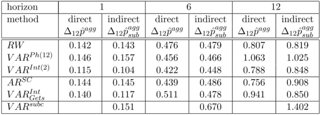
Table 1 presents the comparison of the relative forecast accuracy mea-sured in terms of RMSFE of year-on-year inflation of the direct forecast of aggregate inflation (∆12pˆagg) and the indirect forecast of aggregate inflation,
i.e. the aggregated forecasts of the subindices (∆12pˆaggsub). Graphs comparing actual and forecasted year-on-year inflation as well as tests of equal forecast accuracy are presented to evaluate the economic and statistic significance of the differences between direct and indirect forecasts.
Since different forecast horizons might lead to different rankings of the forecasting methods, the comparison is carried out for short-term to medium-term forecast horizons, 1 to 12 months ahead. In the paper, the results for 1-,6- and 12-months ahead forecasts are presented. The RMSFE evaluation is based on recursive forecasts that involve an average of the respective hori-zon forecasts over all 36 recursive samples.24 The one step ahead forecasts
are starting with the forecast for 1998(2) based on the estimation sample 1992(1) to 1998(1), the second forecast is for 1998(3) based on the estimation sample up to 1998(2), etc., the 36th forecast for 2001(1) is then based on the estimation sample up to 2000(12). Similarly, 12-period-ahead forecasts are carried out for 36 different estimation samples. The forecast for 1999(1) is based on the sample up to 1998(1), whereas the last 12 step ahead forecast is carried out for 2001(12) based on the estimation sample until 2000(12).
Other simulated out-of-sample experiments have been carried out consid-ering 3 subperiods of 12 months of the forecast evaluation period to analyse the sensitivity of the results towards a specific forecast period. The results of this analysis did not change the conclusions of the paper. The focus of the following presentation of the forecast comparison is on the longest forecast evaluation period.
23Note that therefore one source of the resulting forecast error in the simulated
out-of-sample experiment is also the change in subcomponent weights over the forecast horizon. The changes in weights from year to year are relatively small, however.
24Note that in this paper due to the short estimation and forecast evaluation period,
the forecast origins are kept the same for all forecast horizons. Additional forecasts for shorter horizons at a different forecast origin implying different parameter estimates might in this case have a comparatively large impact on the average performance of the different forecast methods.
Relative accuracy of year-on-year inflation forecasts
For a 1-month-ahead forecast horizon aggregating subcomponent forecasts tends to outperform forecasting the aggregate directly in terms of RMSFE for those methods that perform best overall (see Table 1). Whereas for the RW and theARSC both approaches show almost the same performance, for
theV ARP h(12)andV ARsubc(the latter is compared with the direct forecast
based onARSC) the direct forecast of the aggregate is more accurate.
How-ever, for large V ARint(2) and the V ARint
Gets aggregating the subcomponent
forecasts performs better, and those models perform best overall 1-month-ahead. These models are probably better at capturing the increase in energy prices and its second round effects on the other price components as well as the increase in unprocessed food prices in 2000 by explicitly including oil prices, commodity prices and producer prices, among others.
Table 1: Relative forecast accuracy, RMSFE of year-on-year infla-tion in percentage points, Recursive estimainfla-tion samples 1992(1) to 1998(1),...,2000(12)
horizon 1 6 12
method direct indirect direct indirect direct indirect ∆12pˆagg ∆12pˆaggsub ∆12pˆagg ∆12pˆaggsub ∆12pˆagg ∆12pˆaggsub
RW 0.142 0.143 0.476 0.479 0.807 0.819 V ARP h(12) 0.146 0.157 0.456 0.466 1.063 1.025 V ARInt(2) 0.115 0.104 0.422 0.448 0.788 0.848 ARSC 0.144 0.145 0.439 0.486 0.756 0.908 V ARInt Gets 0.140 0.117 0.511 0.478 0.941 0.850 V ARsubc 0.151 0.670 1.402
Note: super and subscripts indicate model selection procedure, SC: Schwarz criterion, Ph(12): Phillips curve model including inflation and unemployment, 12 lags, Int(2): model including international variables in addition to domestic ones, 2 lags, Gets: model selection with PcGets (Hendry & Krolzig, 2001)
In contrast, for a forecast horizon of 6 and 12 months, directly forecasting aggregate inflation tends to perform better in RMSFE terms. TheV ARInt
turns out to be best overall for the period considered forh= 6 for directly as well as indirectly forecasting the aggregate. Forh= 12,RW,V ARint(2)and theV ARint
Gets perform best for the indirect method. The two latter methods
exhibit a very similar forecast accuracy in RMSFE terms. This indicates that taking into account differences in dynamic properties by different model specifications across components in terms of macroeconomic predictors does not improve the accuracy of forecasting aggregate euro area inflation by
aggregating subcomponent forecasts.
The ARSC and the V ARInt(2) model perform better than the other models for the direct method and they also perform best over all direct and indirect methods. TheV ARsubc for indirectly forecasting the aggregate
does perform worse than the direct as well as the indirect method using the ARSC to forecast aggregate inflation 12 months ahead. A possible
ex-planation might relate the RMSFE increase to the estimation uncertainty due to the large number of parameters that is not compensated by taking into account correlations between subcomponents (in first differences) since those are mostly rather small (below 0.25).
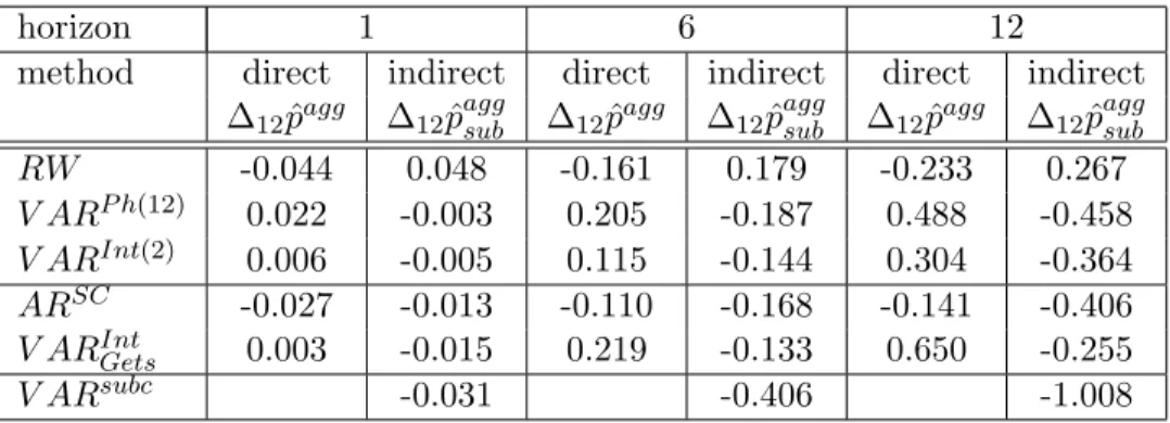
Table 2: Relative forecast accuracy, MFE of year-on-year infla-tion in percentage points, Recursive estimainfla-tion samples 1992(1) to 1998(1),...,2000(12)
horizon 1 6 12
method direct indirect direct indirect direct indirect ∆12pˆagg ∆
12pˆaggsub ∆12pˆagg ∆12pˆaggsub ∆12pˆagg ∆12pˆaggsub
RW -0.044 0.048 -0.161 0.179 -0.233 0.267 V ARP h(12) 0.022 -0.003 0.205 -0.187 0.488 -0.458 V ARInt(2) 0.006 -0.005 0.115 -0.144 0.304 -0.364 ARSC -0.027 -0.013 -0.110 -0.168 -0.141 -0.406 V ARIntGets 0.003 -0.015 0.219 -0.133 0.650 -0.255 V ARsubc -0.031 -0.406 -1.008
Note: super and subscripts indicate model selection procedure, SC: Schwarz criterion, Ph(12): Phillips curve model including inflation and unemployment, 12 lags, Int(2): model including international variables in addition to domestic ones, 2 lags, Gets: model selection with PcGets (Hendry & Krolzig, 2001), subc: all subcomponents as endogenous variables
The average RMSFE for all forecast horizons of 1, 2, 3 etc. up to 12 months ahead (not presented here to save space) has also been calculated to take into account the relative performance of the direct and indirect method for horizons other than the ones presented in Table 1. These average RMSFEs exhibit higher forecast accuracy of the direct forecast method for all models except for the V ARInt
Gets on average over the forecast horizons.
The directV ARInt forecasts are most accurate overall.
The MFE in Table 2 shows that the modulus of the bias of the forecast tends to be lower for those methods that also show a lower RMSFE for the direct or the indirect method, respectively.
The results presented in this section for aggregate HICP suggest that aggregating forecasts of disaggregate components does not necessarily help to forecast the aggregate. The best methods overall exhibit higher forecast
accuracy of directly forecasting aggregate year-on-year inflation over longer horizons, especially for the 12 months horizon of interest for monetary policy.
Do the differences in forecast accuracy matter?
To evaluate how good or bad the alternative methods are in terms of predict-ing year-on-year inflation and how much the direct forecast of the aggregate actually differs from the indirect forecast based on the same method, both forecasts are presented graphically for each method over the 36 recursive samples together with the respective realization.
1999 2000 2001 2002
1 2
3 Random Walk Model
1999 2000 2001 2002
2
4 Phillips Curve VAR
1999 2000 2001 2002 1 2 3 International VAR 1999 2000 2001 2002 1 2 3 Autoregressive Model 1999 2000 2001 2002 1 2 3 PcGets VAR 1999 2000 2001 2002 0 1 2 3 Subcomponent VAR
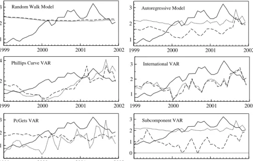
Figure 4: Year-on-year inflation rate and forecasts in %, 12 months ahead, solid: actual, dotted: aggregate forecast, dashed: aggregated subcomponent forecasts
For a one month ahead forecast horizon (the graph is not presented to save space) there are only very small differences between the direct and in-direct approach to forecasting year-on-year inflation for any of the methods. For a forecast horizon of 12 months (see Figure 4), which is more rel-evant for monetary policy, only for the RW a similar result can be seen. In contrast, the ARSC, the V ARP h(12), the V ARInt(2) and the V ARInt
Gets
forecasts differ up to more than 1 percentage points for the direct and indi-rect forecast. The least accurate indiindi-rect forecast based on theV ARsubc is
even 2 percentage points lower than the direct forecast based onARSC. For
the majority of those models that exhibit a relevant difference between the direct and indirect forecast of year-on-year inflation, i.e. ARSC,V ARInt(2)
and V ARInt
Gets, the RMSFE indicates a better performance of forecasting
the aggregate year-on-year inflation directly. The directARSC forecast also outperforms the (indirect)V ARsubc.
The predictive failure of all methods for the 12 months ahead forecast over most of the recursive samples can be explained by their failure to pre-dict several unexpected events: The increase in year-on-year changes of unprocessed food prices since early 2000 due to the effects of weather condi-tions and animal diseases (BSE and Foot-and-Mouth disease); the increase in year-on-year changes of processed food prices over the whole year 2001 due to lagged effects of the animal diseases coming from unprocessed food prices; the increase in year-on-year changes of industrial goods prices in 2001, which is to a large extent due to lagged effects of the increase of en-ergy prices and the depreciation of the euro. Furthermore, the increase in year-on-year changes of energy prices since 1999 and its decline in 2001 is not well captured by either of the methods.
Whether the differences between the direct and the indirect forecasts of year-on-year inflation are statistically significant, has been tested employing the modified version of the Diebold-Mariano test (DMmod) (Diebold &
Mar-iano, 1995) of equal forecast accuracy for non-nested models as suggested by Harvey, Leybourne & Newbold (1997) (referred to as HLN in the follow-ing).25 The test statistic is a small sample correction of the original DM statistic given byDM = ¯d/ q ˆ V( ¯d) with ¯d=N−1PNt=1dˆt, ˆdt= ˆe21t−eˆ22tand V( ¯d) approximately equal to N−1(γ 0+ 2 Ph−1 k=1γk). A consistent estimate
of V( ¯d) is obtained by estimation of the spectrum at frequency zero. West (1996) and McCracken (2000) analyse the effects of parameter estimation uncertainty on tests of equal forecast accuracy for non-nested models. Ac-cording to McCracken (2004) estimation uncertainty can be ignored when the parameters are estimated consistently and the forecast is evaluated by MSFE. Moreover, he finds in simulations that adjustment for parameter un-certainty does not provide much advantage in recursive sampling schemes. The modified DM test has been employed in the current analysis.26,27
It appears that only for the V ARInt(2) the differences between the
di-rect and the indidi-rect forecast 12 months ahead are statistically significant according to this test. To be more precise, the direct forecast is found to be significantly better than the indirect forecast of the aggregate, confirming earlier conclusions. However, the actual forecasts depicted in the graphs suggest an economically relevant difference between the direct and indirect forecasts in particular for theARSC, theV ARInt
Gets and theV ARsubc.
25This test is included following a suggestion by one of the referees. 26The detailed results are available from the author upon request.
27It should be noted that in this study forecast methods not forecast models are
com-pared. Model selection procedures have in principle to be taken into account. However, the relevant theoretical literature is still developing (see e.g. Giacomini & White (2003)).
The results from the modified DM test have to be considered with some caution due to the size and power properties of the test statistic. Harvey et al. (1997) find in their small sample simulation comparison that for a 1-step ahead forecast horizon the test has approximately the right size if the critical values from the t-statistic are used whereas for a horizonh= 10 the even the modified DM test is heavily oversized.28 This implies that the
test might falsely reject equal accuracy of the two forecasts for high forecast horizons. In their power analysis of the modified DM test carried out for 1-step ahead forecasts Harvey et al. (1997) find that for a short forecast evaluation period the power very much depends on the contemporaneous correlation between innovations underlying the forecast errors. Zero or low contemporaneous correlation leads to very low power. Only for very high correlation the power of the test improves.
Overall, the conclusions derived from economic and statistical criteria regarding the significance of the difference between the direct and indirect forecast confirm the results from the RMSFE comparison that the additional effort of modelling subcomponents and aggregating the resulting subcompo-nent forecasts does not necessarily help to increase forecast accuracy when forecasting the aggregate is the objective.
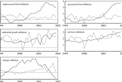
Subcomponent forecasts
Figure 5 shows the results for the V ARint model for each of the
subcom-ponents since this model performs best for the indirect method. It can be seen that unprocessed food, processed food and services inflation are over-predicted in the beginning of the forecast evaluation period, whereas especially unprocessed food and processed food inflation are substantially under-predicted for the whole year of 2001. Energy inflation is substantially over-predicted for the second half of 1999, the year 2000 and the first half of 2001. A similar picture arises for the other models. All forecast models fail badly in predicting the most volatile HICP components,puf andpe.
Ta-ble 3 presents the respective RMSFE per component. Overall, these results provide some explanation why aggregating subcomponent forecasts is not better than forecasting the aggregate inflation rate directly: The subcom-ponents are affected by certain shocks in a similar way and therefore lead to forecast failures in the same direction.
Forecast combination
The results presented so far indicate that it is not necessarily better to ag-gregate subcomponent forecasts, nor is the direct agag-gregate forecast always
28For a forecast evaluation period comparable to the analysis presented in this paper,
1999 2000 2001 2002 0
5 10
unprocessed food inflation
1999 2000 2001 2002
1 2 3 4
processed food inflation
1999 2000 2001 2002
0 1 2
industrial goods inflation
1999 2000 2001 2002 1 2 3 services inflation 1999 2000 2001 2002 0 10 energy inflation
Figure 5: Year-on-year inflation rate in %, solid: actual, dashed: V ARint
sub-component forecast, 12 months ahead
Table 3: Forecasts of HICP (sub-) indices: Forecasting accuracy, RMSFE of year-on-year inflation, forecast horizons: 1 and 12
RW V ARP h(12) V ARInt(2) ARSC V ARInt Gets V ARsubc h=1 puf 0.365 0.502 0.466 0.361 0.418 0.335 ppf 0.119 0.106 0.108 0.098 0.109 0.096 pi 0.106 0.098 0.115 0.100 0.111 0.096 pe 1.442 1.756 1.169 1.493 1.305 1.541 ps 0.149 0.104 0.122 0.097 0.110 0.114 h=12 puf 3.783 4.316 3.998 3.677 3.614 4.038 ppf 1.233 1.229 0.962 1.134 1.092 1.179 pi 0.815 0.570 0.534 0.473 0.552 0.469 pe 7.957 12.477 8.622 8.196 8.353 8.635 ps 1.409 0.604 0.592 0.532 0.776 0.943
Note: super and subscripts indicate model selection procedure, SC: Schwarz criterion, Ph(12): Phillips curve model including inflation and unemployment, 12 lags, Int(2): model including international variables in addition to domestic ones, 2 lags, Gets: model selection with PcGets (Hendry & Krolzig, 2001), subc: all subcomponents as endogenous variables
better. Therefore, the forecast accuracy of combinations of direct and indi-rect methods of forecasting the aggregate 12 months ahead are investigated in this section. Additionally it is explored whether pooling subcomponent forecasts provides a more robust forecasting method for forecasting the sub-components leading to a more accurate indirect aggregate forecast.
A comprehensive discussion of different methods of forecast combination would go beyond the scope of the paper. A discussion of the different forecast combination methods and review of the literature can be found, among others, in Clemen (1989), Diebold & Lopez (1996) and Clements & Hendry (2004).
It should be noted that in principle the aggregation of subcomponent forecasts is a way of forecast combination. As discussed above, combin-ing the subcomponent forecasts does not help to forecast the aggregate 12 months ahead since forecasts will fail in the same direction when an unex-pected shock occurs that is affecting some or all forecasts to be combined. Similarly, one might expect that combining the direct and indirect meth-ods would not necessarily improve forecast accuracy. On the other hand, combination of forecasts can improve the overall forecasts if models provide partial explanations, especially if forecasts are differentially biased (one is biased upward, one downward). Furthermore, variance reduction can be achieved by using various information sets efficiently. Sample estimation uncertainty will also influence the relative forecast accuracy. Whether fore-cast combination is an improvement on the separate forefore-casts in the present case is an open question we study below.
RMSFEs are calculated for a number of combined forecasts of euro area inflation 12 months ahead. Simple (mean) averaging is employed since that is often found to perform better than more sophisticated methods (see e.g. Clements & Hendry (2004), Stock & Watson (2003)). Pooled forecasts might provide a more robust forecasting tool for the subcomponents and this is investigated. I combine the 4 best out of 6 forecasts, i.e. discarding 1/3 of the worst forecasts, for each of the subcomponents. The resulting combined forecasts are then aggregated. The RMSFE for this forecast combination method is 0.755. This is clearly an improvement over all other indirect forecast methods of the aggregate (Table 1). In comparison with the forecast accuracy of the direct forecasts, this combination method is very similar to the best direct forecast, theARSC. Thus, despite a large effort in modelling and forecasting disaggregate components, this forecast combination method hardly improves over the best direct method in terms of forecast accuracy measured by the RMSFE.
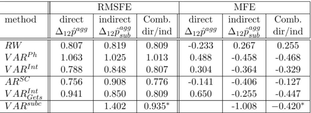
Another direction for exploring the performance of forecast combination in the present context is the following: Since neither the direct nor the indi-rect forecast of the aggregate is always better than the other, it is of interest to investigate whether taking into account the disaggregate dynamics in a combined forecast of the direct and indirect method improves the forecast
accuracy over the direct forecast and thus justifies the additional investment of modelling subcomponents when forecasting the aggregate is the objective. For five out of the six methods considered in this analysis, the direct and the indirect forecasts are actually biased in the opposite direction for 12 months ahead forecasts (see Table 2). Thus, the direct and indirect forecast for each method are combined and the respective RMSFE are presented in Table 4. Forecast combination does not improve the RMSFE over the best forecast for the respective method except forV ARP h(12)and V ARInt
Gets (see
Table 4). There is no improvement over the best forecast 12 months ahead overall. In an alternative approach, the two best forecast methods for the indirect forecast are combined and compared with the two best combined forecast methods for the direct forecast 12 months ahead. More precisely, since for the indirect forecast the RW and the V ARint(2) perform best in
RMSFE terms (Table 4), but exhibit a bias in opposite direction, those two methods are combined. For the direct forecast the V ARint(2) and the
ARSC are combined since those methods perform best in RMSFE terms.
V ARint(2) has a positive bias whereas ARSC exhibits a negative bias.
Focast combination does indeed lead to some improvement over the best re-spective forecast for both the direct and the indirect method. However, the combined direct forecast still performs best overall for the forecast combina-tions chosen (RMSFE: 0.719). It should be noted that the methods chosen for forecast combination in this case are selected based on the same forecast evaluation period as their final evaluation due to the short sample available. Alternatively, all direct and indirect forecast methods considered in this study are combined. The resulting forecast is better in RMSFE terms 12 months ahead (0.722) than any of the direct or indirect methods separately.
HICP excluding energy and unprocessed food
Another aggregate inflation measure that is of interest for the ECB is HICP inflation excluding energy and unprocessed food, sometimes referred to as ’core’ inflation. The results in terms of the RMSFE of year-on-year ’core’ inflation are presented in Table 5.
Here the results show a different pattern than for forecasting aggregate HICP inflation including all components. Three out of six methods exhibit a better accuracy for aggregating the subcomponent forecasts for a forecast horizon of 1, 6 and 12 months, i.e. all methods except for the RW, the V ARInt
Gets and the V ARsubc. The results for V ARIntGets in comparison with
theV ARInt in Table 5 also show that for the three components the varying
specification across components in terms of variables chosen to be included in the VAR does not improve but worsens the forecast accuracy of aggregating the subcomponent forecasts. Graphs (not presented here to save space) of the direct and indirect year-on-year inflation forecasts 12 months ahead show that theV ARint(2) method exhibits similar aggregate forecasts based on the
Table 4: Relative forecast accuracy, RMSFE and MFE of the di-rect, indirect and combination forecasts, 12 months ahead, year-on-year inflation in percentage points, Recursive estimation sam-ples 1992(1) to 1998(1),...,2000(12)
RMSFE MFE
method direct indirect Comb. direct indirect Comb.
∆12pˆagg ∆
12pˆaggsub dir/ind ∆12pˆagg ∆12pˆaggsub dir/ind
RW 0.807 0.819 0.809 -0.233 0.267 0.255 V ARP h 1.063 1.025 1.013 0.488 -0.458 -0.468 V ARInt 0.788 0.848 0.807 0.304 -0.364 -0.329 ARSC 0.756 0.908 0.776 -0.141 -0.406 -0.127 V ARInt Gets 0.941 0.850 0.809 0.650 -0.255 -0.447 V ARsubc 1.402 0.935∗ -1.008 −0.420∗
Note: super and subscripts indicate model selection procedure, SC: Schwarz criterion, Ph: Phillips curve model including inflation and unemployment, 12 lags, Int: model including international variables in addition to domestic ones, 2 lags, Gets: model selection with PcGets (Hendry & Krolzig, 2001), subc: all subcomponents as endogenous variables, ∗
indicates combination withARSC
Table 5: Relative forecast accuracy, RMSFE of year-on-year inflation of HICP excluding unprocessed food and energy in percentage points, Recursive estimation samples 1992(1) to 1998(1),...,2000(12)
horizon 1 6 12
method direct indirect direct indirect direct indirect
∆12pˆcore ∆
12pˆcoresub ∆12pˆcore ∆12pˆcoresub ∆12pˆcore ∆12pˆcoresub
RW 0.103 0.105 0.551 0.565 1.068 1.097 V ARP h(12) 0.065 0.060 0.244 0.226 0.584 0.570 V ARInt(2) 0.078 0.075 0.281 0.264 0.525 0.490 ARSC 0.061 0.055 0.237 0.226 0.520 0.501 V ARIntGets 0.064 0.064 0.271 0.294 0.574 0.672 V ARsubc 0.063 0.256 0.548
Note: super and subscripts indicate model selection procedure, SC: Schwarz criterion, Ph(12): Phillips curve model including inflation and unemployment, 12 lags, Int(2): model including international variables in addition to domestic ones, 2 lags, Gets: model selection with PcGets (Hendry & Krolzig, 2001), subc: all subcomponents as endogenous variables
direct and indirect method for some periods. In contrast, the difference for the other models is up to 0.8 percentage points. These findings indicate that the better RMSFE accuracy for the indirect method of aggregating subcomponent forecasts matters from a policy perspective with respect to the actual ’core’ inflation forecast.
The analysis reveals that the ’core’ inflation series including only those subindices of HICP that are less affected by shocks tends to be better fore-casted by aggregating the subcomponent forecasts. This is in contrast to the year-on-year inflation rate of HICP total that tends to be better forecasted directly over longer horizons.
6
Conclusions: Why does disaggregation not
nec-essarily help?
In this study a simulated out-of-sample experiment is carried out to compare the relative forecast accuracy of aggregating the forecasts of euro area sub-component inflation (’indirect’ method) as opposed to forecasting aggregate euro area year-on-year inflation directly (’direct’ method) in terms of their RMSFE. This study covers a broad range of models and model selection procedures.
I find that it is not necessarily better to employ the indirect rather than the direct method. For many of the forecast methods considered here that are often used by practitioners and researchers, forecasting aggregate euro area year-on-year inflation directly results in higher forecast accuracy for the medium-term forecast horizons of 12 months that are relevant for monetary policy.
Furthermore, the combination of different forecast methods for subcom-ponents as well as most of the combinations of direct and indirect forecasts are not found to improve over the best (direct) forecast 12 months ahead. The findings suggest that methods that only rely on aggregating subcom-ponent forecasts have to be considered with some caution, even when the dynamic properties of subcomponents have been taken into account by dif-ferent model specifications. Thus, for forecasting year-on-year inflation in the euro area the results presented raise the question whether modelling and forecasting the subcomponents is worthwhile if the forecast of the aggregate is the objective.
Although the details of the results in this study are of course specific to the empirical application of euro area inflation, the findings nevertheless point at some more general problems the forecaster may face when aggre-gating forecasts of disaggregate components to forecast the aggregate.
The forecast errors of the subcomponents of the euro area HICP do not cancel. This is because many shocks, e.g. the oil price shock or the shocks to unprocessed food in 2000 and 2001 in the euro area, affect several or
even all components of HICP in a similar way over the forecast evaluation period. Thus, the forecast bias is not reduced but increased by aggregating the subcomponent forecasts.
Furthermore, I have investigated the forecast performance of aggregating subcomponent forecasts for another inflation measure of interest to mone-tary policy makers: inflation excluding unprocessed food and energy prices, sometimes referred to as ’core’ inflation. The results are more favorable for aggregating subcomponent forecasts than in the analysis for overall HICP inflation. For this aggregate the best methods exhibits higher forecast ac-curacy for aggregating subcomponent forecasts. Comparing these findings with the results for overall year-on-year inflation sheds further light regard-ing the problems of aggregatregard-ing subcomponent forecasts. Aggregatregard-ing sub-component forecasts appears to be problematic when some sub-components are inherently difficult to forecast as is the case with energy and unprocessed food prices.
References
Angelini, E., Henry, J. & Mestre, R. (2001). Diffusion index-based inflation forecasts for the euro area,ECB Working Paper 61, European Central Bank.
Barker, T. & Pesaran, M. H. (1990a). Disaggregation in econometric mod-elling, Routledge, London and New York.
Barker, T. & Pesaran, M. H. (1990b). Disaggregation in econometric mod-elling - an introduction, inT. Barker & M. H. Pesaran (eds), Disaggre-gation in econometric modelling, Routledge, London and New York. Canova, F. (2002). G7 inflation forecasts, ECB Working Paper 151,
Euro-pean Central Bank.
Clemen, R. T. (1989). Combining forecasts: A review and annotated bibli-ography,International Journal of Forecasting 5: 559–583.
Clements, M. P. & Hendry, D. F. (1998).Forecasting Economic Time Series, Cambridge University Press, Cambridge, UK.
Clements, M. P. & Hendry, D. F. (1999). Forecasting Non-stationary Eco-nomic Time Series, MIT Press, Cambridge,Massechusetts.
Clements, M. P. & Hendry, D. F. (2002). Modelling methodology and fore-cast failure, Econometrics Journal 5: 319–344.
Clements, M. P. & Hendry, D. F. (2004). Pooling forecasts, Econometrics Journal, forthcoming.
Cristadoro, R., Forni, M., Reichlin, L. & Veronese, G. (2001). A core infla-tion index for the euro area, Temi di Discussione 435, Banca d’Italia. Diebold, F. X. & Kilian, L. (2000). Unit-root tests are useful for
select-ing forecastselect-ing models, Journal of Business & Economic Statistics
18(3): 265–272.
Diebold, F. X. & Lopez, J. A. (1996). Forecast evaluation and combination, in G. Maddala & C. Rao (eds),Handbook of Statistics, Vol. 14, North-Holland, Amsterdam, pp. 241–268.
Diebold, F. X. & Mariano, R. S. (1995). Comparing predictive accuracy, Journal of Business & Economic Statistics 13(3): 253–263.
Espasa, A., Senra, E. & Albacete, R. (2002). Forecasting inflation in the European Monetary Union: A disaggregated approach by countries and by sectors,European Journal of Finance 8(4): 402–421.
European Central Bank (2000). ECB Monthly Bulletin, December. European Central Bank (2003a). ECB Monthly Bulletin, March.
European Central Bank (2003b). ECB Press Release, The ECB’s monetary policy strategy, 8 May 2003, Press Release, http://www.ecb.int. Fair, R. C. & Shiller, J. (1990). Comparing information in forecasts from
econometric models, The American Economic Review 80(3): 375–389. Giacomini, R. & White, H. (2003). Tests of conditional predictive ability,
Working Paper 272, University of California, San Diego.
Granger, C. W. J. (1990). Aggregation of time-series variables: A survey, in T. Barker & M. H. Pesaran (eds), Disaggregation in econometric modelling, Routledge, London and New York, pp. 17–34.
Granger, C. W. J. & Morris, M. J. (1976). Time series modelling and interpretation, Journal of Royal Statistical Society 139: 246–257. Grunfeld, Y. & Griliches, Z. (1960). Is aggregation necessarily bad?, The
Review of Economics and StatisticsXLII(1): 1–13.
Harvey, D., Leybourne, S. & Newbold, P. (1997). Testing the equality of prediction mean squared errors, International Journal of Forecasting
13: 281–291.
Hendry, D. F. & Clements, M. P. (2003). Economic forecasting: Some lessons from recent research, Economic Modelling(20): 301–329.
Hendry, D. F. & Krolzig, H.-M. (2001). Automatic Econometric Model Se-lection Using PcGets 1.0, Timberlake Consultants Ltd., London, UK. Hendry, D. F. & Krolzig, H.-M. (2003). New developments in automatic
general-to-specific modelling, inB. P. Stigum (ed.), Econometrics and the Philosophy of Economics. Theory-Data Confrontations in Eco-nomics, Princeton University Press, Princeton.
Inoue, A. & Kilian, L. (2003). On the selection of forecasting models,ECB Working Paper 214, European Central Bank.
Kohn, R. (1982). When is an aggregate of a time series efficiently forecast by its past?, Journal of Econometrics(18): 337–349.
Leamer, E. E. (1990). Optimal aggregation of linear net export systems, in T. Barker & M. H. Pesaran (eds), Disaggregation in econometric modelling, Routledge, London and New York, pp. 150–170.
Lippi, M. & Forni, M. (1990). On the dynamic specification of aggregated models, in T. Barker & M. H. Pesaran (eds),Disaggregation in econo-metric modelling, Routledge, London and New York, pp. 150–170. L¨utkepohl, H. (1984a). Forecasting contemporaneously aggregated vector
ARMA processes,Journal of Business & Economic Statistics2(3): 201– 214.
L¨utkepohl, H. (1984b). Linear transformations of vector ARMA processes, Journal of Econometrics(26): 283–293.
L¨utkepohl, H. (1987). Forecasting Aggregated Vector ARMA Processes, Springer-Verlag.
Marcellino, M. (1999). Some consequences of temporal aggregation in em-pirical analysis,Journal of Business & Economic Statistics17(1): 129– 136.
Marcellino, M. (2004). Forecasting EMU macroeconomic variables, Inter-national Journal of Forecasting 20(2): 359–372.
Marcellino, M., Stock, J. H. & Watson, M. W. (2003). Macroeconomic fore-casting in the euro area: Country specific versus area-wide information, European Economic Review 47: 1–18.
McCracken, M. (2000). Robust out-of-sample inference, Journal of Econo-metrics99: 195–223.
McCracken, M. (2004). Parameter estimation and tests of equal forecast accuracy between non-nested models, International Journal of Fore-casting, forthcoming.
Nijman, T. & Sentana, E. (1996). Marginalization and contemporaneous aggregation in multivariate garch processes, Jounal of Econometrics
71: 71–87.
Pesaran, M. H., Pierse, R. G. & Kumar, M. S. (1989). Econometric analysis of aggregation in the context of linear prediction models,Econometrica
57: 861–888.
Rose, D. E. (1977). Forecasting aggregates of independent ARIMA pro-cesses,Journal of Econometrics (5): 323–345.
Stock, J. H. & Watson, M. W. (1996). Evidence on structural instability in macroeconomic time series relations, Journal of Business & Economic Statistics 14(1): 11–30.
Stock, J. H. & Watson, M. W. (1999). Forecasting inflation, Journal of Monetary Economics44: 293–335.
Stock, J. H. & Watson, M. W. (2003). Combination forecasts of output growth in a seven-country data set, manuscript.
Theil, H. (1954).Linear Aggregation of Economic Relations, North Holland, Amsterdam.
Tiao, G. C. & Guttman, I. (1980). Forecasting contemporal aggregates of multiple time series, Journal of Econometrics(12): 219–230.
Van Garderen, K. J., Lee, K. & Pesaran, M. H. (2000). Cross-sectional aggregation of non-linear models, Journal of Econometrics 95: 285– 331.
Wei, W. W. S. & Abraham, B. (1981). Forecasting contemporal time se-ries aggregates, Communications in Statistics - Theory and Methods
A10: 1335–1344.
West, K. D. (1996). Asymptotic inference about predictive ability, Econo-metrica 64: 1067–1084.
Zellner, A. & Tobias, J. (2000). A note on aggregation, disaggregation and forecasting performance, Journal of Forecasting19: 457–469.