Forecasting euro area inflation using dynamic factor measures of underlying inflation

W O R K I N G PA P E R S E R I E S

N O. 4 0 2 / N OV E M B E R 2 0 0 4

FORECASTING EURO

AREA INFLATION

USING DYNAMIC

FACTOR MEASURES

OF UNDERLYING

INFLATION

In 2004 all publications will carry a motif taken from the €100 banknote.

W O R K I N G PA P E R S E R I E S

N O. 4 0 2 / N OV E M B E R 2 0 0 4

FORECASTING EURO

AREA INFLATION

USING DYNAMIC

FACTOR MEASURES

OF UNDERLYING

INFLATION

and George Kapetanios

This paper can be downloaded without charge from http://www.ecb.int or from the Social Science Research Network electronic library at http://ssrn.com/abstract_id=601022.

é

© European Central Bank, 2004 Address

Kaiserstrasse 29

60311 Frankfurt am Main, Germany Postal address

Postfach 16 03 19

60066 Frankfurt am Main, Germany Telephone +49 69 1344 0 Internet http://www.ecb.int Fax +49 69 1344 6000 Telex 411 144 ecb d

All rights reserved.

Reproduction for educational and non-commercial purposes is permitted provided that the source is acknowledged.

The views expressed in this paper do not necessarily reflect those of the European Central Bank.

C O N T E N T S

Abstract 4

Non-technical summary 5

1 Introduction 6

2 Dynamic factor method 8

2.1 Dealing with large datasets 10

3 Measures of underlying inflation 11

4 Data and empirical results 14

4.1 Data 14

4.2 Empirical results 15

5 Conclusion 17

References 19

Tables an figures 22

Abstract

Standard measures of prices are often contaminated by transitory shocks. This has prompted economists to suggest the use of mea-sures of underlying inflation to formulate monetary policy and assist in forecasting observed inflation. Recent work has concentrated on In this paper we esti-mate factors from datasets of disaggregated price indices for European countries. We then assess the forecasting ability of these factor esti-mates against other measures of underlying inflation built from more traditional methods. The power to forecast headline inflation over horizons of 12 to 18 months is adopted as a valid criterion to assess forecasting. Empirical results for the five largest euro area countries as well as for the euro area are presented.

JEL-classification: E31, C13, C32.

modelling large datasets using factor models.

Non-technical summary

The aim of monetary policy in most modern economies is maintaining price stability over the medium term. A common problem faced by those respon-sible for monetary policy decisions is that standard measures of prices are often contaminated by three main types of transitory shocks: i) measurement errors, ii) regular seasonal fluctuations, and iii) other non-monetary factors, such as for example a good or bad harvest. This has prompted economists to suggest the use of ‘filtered’ versions of published price indexes as measures of underlying inflation.

Two major approaches for filtering a price index have been tradition-ally adopted. The first approach exploits the cross section dimension, and relies on modifying the weights attached to the different subcomponents of consumer price indexes. The weights are modified so that the more volatile subcomponents of consumer price indexes are either set to zero or assigned smaller values. The second approach exploits the time series dimension of the aggregate price index series, and builds a measure of underlying inflation at a point in time as the weighted sum of observations from the past and the future. The aim of this approach is to isolate the persistent component of aggregate inflation, i.e. that component that does not vanish in future periods but leaves a permanent mark.

In recent work, Kapetanios (2002) proposed a new method of estimating dynamic factor models that exploits both the cross section dimension and the time series dimension. This method is easy to implement and can also accommodate cases where the number of variables exceeds the number of observations. This method forms part of a large set of algorithms used in the engineering literature for estimating state space models called subspace algorithms.

This paper presents an assessment of the reliability of measures of under-lying inflation built from subspace algorithms against other measures built from more traditional methods. The power to forecast headline inflation over horizons of 12 to 18 months is adopted as a valid criterion to assess reliabil-ity. Empirical results for the five largest euro area countries as well as for the euro area are presented. Results show that measures of core inflation built by means of dynamic factor methods perform well in comparison to traditional measures. This paper also warns that measures of underlying inflation based on methods that ignore the time series dimension of price indexes may fail to cointegrate with headline inflation.

1

Introduction

Monetary policy in most modern economies aims at maintaining price sta-bility over the medium term. A common problem faced by those responsible for monetary policy decisions is that standard measures of prices are often contaminated by three main types of transitory shocks: i) measurement er-rors, ii) regular seasonal fluctuations, and iii) other non-monetary factors, such as for example a good or bad harvest. This has prompted economists to suggest the use of ‘filtered’ versions of published price indexes as measures of underlying inflation, see for example Bryan and Cecchetti (1994) and Vega and Wynne (2001).

Two major approaches for filtering a price index have been adopted. The first approach exploits the cross section dimension, and in effect acts upon the original series by modifying the weights attached to its different subcom-ponents. An example in this vein is a study conducted for the euro area HICP by Vega and Wynne (2001) which suggested that a trimmed mean measure of underlying inflation outperforms a measure computed by excluding un-processed food and energy prices. The second approach exploits the time series dimension of the price index series, and builds a measure of underlying inflation at a point in time as the weighted sum of observations from the past and the future. The justification for this approach follows the suggestion by Blinder (1997) to identify the persistent component of aggregate inflation as an underlying measure of inflation, i.e. that component that does not vanish in future periods but leaves a permanent mark. Bryan and Cecchetti (1993) were the first to propose a method that exploit both the cross section as well as the time series dimension. They proposed to model a vector of subcomponents of the US Consumer Price Index (CPI) by means of a dy-namic factor index model. This model has a state space representation, and maximum likelihood methods in combination with the Kalman filter can be implemented to estimate the unknown parameters, along the lines explained in Harvey (1993).1

However, maximum likelihood estimation of a state space model is not practical when the dimension of the model becomes too large due to the com-putational cost. The modelling strategy proposed by Bryan and Cecchetti (1993) is therefore difficult to implement for levels of disaggregation of the subcomponents of the price index finer than the two-digit level. Additionally, their method can not be implemented when the number of observations is smaller than the number of price subcomponents employed. In recent work, Kapetanios (2004) has proposed a new method of estimating factor models based on subspace algorithms that also exploits both the cross section dimen-sion and the time series dimendimen-sion and, importantly, the method does not require iterative estimation techniques. This makes possible a high degree of disaggregation of the price index series. This method can also accommodate cases where the number of variables exceeds the number of observations as shown also in Kapetanios (2004). The method forms part of a large set of al-gorithms used in the engineering literature for estimating state space models called subspace algorithms.

This paper presents an assessment on the reliability of measures of under-lying inflation built from subspace algorithms against other measures built from more traditional methods. The power to forecast headline inflation over horizons of 12 to 18 months is adopted as a valid criterion to assess reliabil-ity.2 Empirical results for the five largest euro area countries as well as for the euro area are presented.

The method proposed by Kapetanios (2004) is described in section 2. Section 3 describes a variety of methods used in the literature to compute measures of underlying inflation. The methods reviewed in this section will be referred to as ‘traditional’ methods in this paper. Section 4 provides details

2_{Vega and Wynne (2001) suggested also the ability to track trend inflation as a criterion}

on the nature of the forecasting exercise conducted to assess the reliability of different measures of underlying inflation and presents the empirical results. Finally, section 5 concludes.

2

Dynamic Factor Method

We consider the following state space model.

xt = Cft+Dut, t= 1, . . . , T

ft = Aft−1+But−1 (1)

xt is an n-dimensional vector of strictly stationary zero-mean variables ob-served at time t. f_tis an m-dimensional vector of unobserved states (factors) at time t and u_t is a multivariate standard white noise sequence of dimen-sion n. The aim of the analysis is to obtain estimates of the states f_t, for

t = 1, . . . , T. This state space model may not appear familiar as the presence

of the same error term in both the transition and measurement equations is non-standard. However, as Hannan and Deistler (1988, Ch. 1) show, (1), referred to as the prediction error representation of the state space model, is equivalent to the following more common representation

xt = Cft+D∗ut, t= 1, . . . , T (2)

ft = Aft−1+B∗vt−1

where u_t and v_t are multivariate standard orthogonal white noise sequences. We concentrate on (1) as it forms the basis for deriving the dynamic factor estimation algorithm.

Subspace algorithms avoid expensive iterative techniques and rely instead on matrix algebraic methods to provide estimates for the factors as well as the parameters of the state space representation. A review of existing subspace algorithms is given by Bauer (1998) in an econometric context. Another review with an engineering perspective may be found in Overschee and Moor (1996).

The starting point of most subspace algorithms is the following represen-tation of the system which follows from the state space represenrepresen-tation (2) and the assumed nonsingularity of D.

X_tf =OKX_tp+EE_tf (3) where X_tf = (x_t, x_t+1, x_t+2, . . .), X_tp = (x_t−1, x_t−2, . . .), E_tf = (u_t, u_t+1, . . .), O = [C, AC,(A2)C, . . .] K = [ ¯B,(A−BC¯ ) ¯B,(A−BC¯ )2B, . . .¯ ] where ¯B =BD−1 and E =       D 0 . . . 0 CB D . .. ... CAB . .. ... 0 .. . CB D      

The derivation of this representation is easy to see once we note that (i)

X_tf =Of_t+EE_tf and (ii)f_t=KX_tp. The best linear predictor of the future of the series at time t is given by OKX_tp. The state is given in this context by KX_tp at time t. The task is therefore to provide an estimate for K. Ob-viously, the above representation involves infinite dimensional vectors.

In practice, truncation is used to end up with finite sample approxima-tions given byX_s,tf = (x_t, x_t+1, x_t+2, . . . , x_t+s−1)andX_q,tp = (x_t−1, x_t−2, . . . , x_t−q). Then an estimate of F = OK may be obtained by regressing X_s,tf on X_q,tp . Following that, the most popular subspace algorithms use a singular value decomposition of an appropriately weighted version of the least squares es-timate of F, denoted by ˆF. In particular the algorithm we will use, due to Larimore (1983), applies a singular value decomposition to ˆΓf−1/2FˆΓˆp1/2, where ˆΓf, and ˆΓp are the sample covariances of X_s,tf and X_q,tp respectively. These weights are used to determine the importance of certain directions in

ˆ

F. Then, the estimate of K is given by ˆ

where ˆUSˆVˆ represents the singular value decomposition of ˆΓf−1/2FˆΓˆp1/2, ˆV_m denotes the matrix containing the first m columns of ˆV and ˆS_m denotes the headingm×msubmatrix of ˆS. ˆScontains the singular values of ˆΓf−1/2FˆΓˆp1/2 in decreasing order. Then, the factor estimates are given by ˆKX_tp. More de-tails on the method, including its asymptotic properties, may be found in Kapetanios and Marcellino (2003). Once an estimate of the factor is ob-tained then the parameters of the state space model may be estimated using standard regression techniques and the factor estimates in the measurement and transition equations. Thus, it is possible to produce forecasts for the factors.

2.1

Dealing with large datasets

Up to now we have outlined an existing method for estimating factors which requires that the number of observations be larger than the number of el-ements in X_tp. Given the work of Stock and Watson (2002), on modelling very large datasets with factor models, this is rather restrictive. We therefore follow Kapetanios and Marcellino (2003) who suggested a modification of the existing methodology to allow the number of series in X_tp be larger than the number of observations. The problem arises in this method because the least squares estimate ofF does not exists due to rank deficiency of XpXp where

Xp _{= (X}p

1, . . . , XTp). As we mentioned in the previous section we do not

necessarily want an estimate of F but an estimate of the states XpK. That could be obtained if we had an estimate of XpF and used a singular value decomposition of that. But it is well known (see e.g. Magnus and Neudecker (1988)) that although ˆF may not be estimable XpF always is using least squares methods. In particular, the least squares estimate of XpF is given by

Xp_{F =X}p_(Xp

Xp₎+_Xp

Xf

where Xf = (X₁f, . . . , X_Tf) and A+ denotes the unique Moore-Penrose in-verse of matrix A. Once this step is modified then the estimate of the factors

may be straightforwardly obtained by applying a singular value decompo-sition to XpF. Kapetanios (2004) chooses to set both weighting matrices to the identity matrix in this case. In our results below we will pursue two alternative subspace methods. Method 1, denoted in the tables below as SS1, relies on the singular value decomposition of Xp(XpXp)+XpXf = ˆUSˆVˆ. Then, the factor estimates are given by ˆU_mSˆ_m1/2. Method 2, denoted SS2, relies on the singular value decomposition of (XpXp)+XpXf = ˆUSˆVˆ. Here the factor estimates are given by XpUˆ_mSˆ_m1/2. Note that Xp(XpXp)+Xp =I when the number of columns of Xp exceeds its number of rows. We there-fore see that SS1 essentially decomposes Xf, and resembles the approximate dynamic factor methodology of Stock and Watson (2002) based on principal components. The SS2 method, on the other hand is genuinely dynamic in that it exploits the dynamic relationship between Xf andXp to estimate the factor.

3

Measures of Underlying Inflation

Headline inflation will be defined asπ_t = 100 ln(P_t/P_t−12), whereP_tis a price index measure. For our purposes, we defined n as the number of subcompo-nents of the price measure, and w_i for i = 1 to n as the weights associated with the i-th subcomponent, it follows that P_t = n_i=1w_iP_i,t where P_i,t is the price index for subcomponent i at time t.

Dynamic factor measures. Dynamic factor measures of underlying in-flation are built from a state space system such as that in (1), where x_t is defined as a n×1 vector with elementsx_i,t = 100 ln(P_i,t/P_i,t−12) for i= 1 to

n. The measure of underlying inflation is the first factor estimate of ˆFX_tp. As stated above, when the estimate of this first factor relies on a singular value decomposition of Xp(XpXp)+XpXf, this will be denoted by SS1 in our empirical results below, and when the first factor relies on a singular value decomposition of (XpXp)+XpXf, this will be denoted by SS2.

Excluding measures. These measures simply exclude certain subcompo-nents of the price index to compute a core inflation measure. This translates into zeroing out some of the weights w_i, and scaling the non-zero weights so that they add to one, these newly defined weights, say ˜w_i are then used to compute a new aggregate price index, ˜P_t = p_i=1w˜_iP_i,t for p < n. Four measures, corresponding to four alternative weightings will be tested in this paper. These are defined as follows: i) EX1, excludes the energy compo-nents; ii) EX2, excludes energy and food compocompo-nents; iii) EX3, excludes energy and unprocessed food components; and iv) EX4, excludes energy and seasonal food components. Additionally, and following ECB (2004, pp. 27-28) we build a measure that aims at excluding components whose prices are subject to a certatin degree of government control; i.e. this measure excludes administered prices. We will denote this measure as ADM.3

Trimmed Mean measures. Define the headline ‘ordered’ rate of inflation as: π_to = n_j=1w_joπo_j,t for j = 1 to n, where the inflation rate for the sub-components, π_j,to , are ‘ordered’ from smallest to largest, and w_jo define their corresponding weights. A trimmed measure of inflation is then defined as follows: π2α t = 1 1−2α n−p j=m+1 wo jπj,to

where m and p are chosen such that m_j=1w_jo =n_j=n−p+1w_jo =α. We have defined a total of 6 trimmed measures of underlying inflation, with the size of the trimming (2α) ranging between values of 1% to 50%. These measures are denoted as: TR1, TR5, TR10, TR20, TR30 and TR50. Note that the median in effect can be seen as a trimmed measure, that trims 50% on the left and 50% on the right. We denote the underlying measure of inflation built from the median as MED.

3_{The ADM measure excludes: tobacco, energy, sewerage collection, refuse collection,}

medical and paramedical services, dental services, hospital services, passenger transport by railway, postal services, education and social protection.

Edgeworth Index. This measure is defined as EDGE = n_j=1we_jπ_j,t for

j = 1 ton, where the weights w_je are inversely related to the volatility ofπ_j,t, and defined as follows:

we j = σ−2 i,t _n j=1σj,t−2 where E(π_j,t−Eπ_j,t)2 =σ_j,t2 .

Unobserved Component model measure. We adopt the unobserved component (UC) model proposed by Harvey and Jaeger (1993) to extract a measure of underlying inflation. This measure exploits only the time series dimension.

πt=µt+γt+εt

whereµ_tis a trend component,γ_tis a cyclical component and ε_tan irregular noise component with standard deviation σ_ε. The trend component µ_t is for our purposes a measure of underlying inflation, and will be referred to as the UC measure of underlying inflation in this paper. Details on the structure of the trend component µ_t and the stochastic cycleγ_tcan be found in Harvey and Jaeger (1993). The model can be written in State Space form and the Kalman filter implemented to extract the state component. Given that there are parameters to be estimated, maximum likelihood estimation in combination with the Kalman filter must be used.

Quah and Vahey (1995) measure. Quah and Vahey (1995) provided a method to construct a measure of underlying inflation by placing dynamic restrictions on a vector autorregression (VAR) system with ∆y and ∆π as endogenous variables, whereydenotes the logarithm of industrial production. They adopt an identification strategy similar to that in Blanchard and Quah (1989), by which they assume that the first kind of disturbance has no impact on output in the long run. Underlying inflation is defined as the movements in inflation associated with this first disturbance. This measure will be denoted as QV in the paper.

4

Data and Empirical Results

4.1

Data

Our empirical results will be conducted for the euro area (EA), and the largest five countries of the euro area in terms of GDP; namely Germany (DE), France (FR), Italy (IT), The Netherlands (NL) and Spain (SP). The Harmonised Index of Consumer Prices (HICP) is therefore the obvious choice of price measure to use. One of the principle objectives of the European Union is to promote economic and social progress, and in order to conduct its policies, there is a need for monitoring the economic performance across countries. This can only be achieved if the available statistical information is comparable.

Work on the harmonisation of consumer price indices across EU coun-tries started in 1993, and by March 1997 the first figures of a harmonised index of consumer prices (HICP) for each member state were being published. The HICP has been designed to ensure the comparability of consumer price indices across EU countries. Eugenio Domingo Solans (member of the Exec-utive Board of the ECB) has pointed out that the HICP was the only serious contender for the measurement of inflation in 1998, see Solans (2001). He further stated that from the perspective of the ECB, the HICP possesses some very attractive qualities. First, it covers a large proportion of house-hold expenditure. Second, it is available monthly and in a timely manner. Third, it is aggregable in the sense that the country pieces fit together with-out gaps or overlaps. Four, it is subject to only minor revisions. Finally, it is based on actual monetary transactions. These features and the fact that it is comparable across countries, and can therefore be aggregated, makes the HICP the optimal choice for monitoring price developments in euro area countries.

4.2

Empirical Results

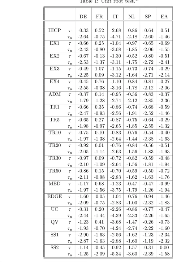
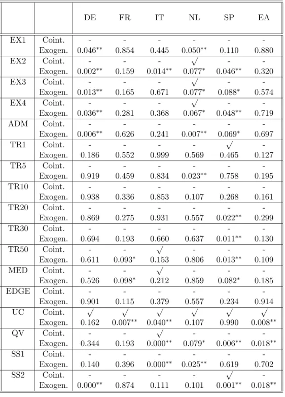
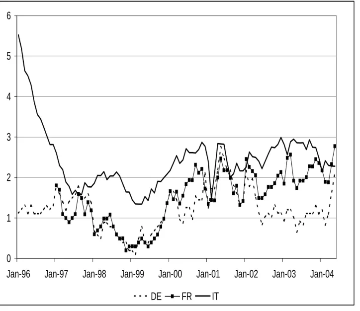
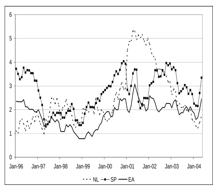
Figures 1 and 2 display the year on year changes in % the HICP for the euro area and largest five countries of the euro area, which we define in this paper as the measure of headline inflation. Table 1 shows the Augmented Dickey-Fuller statistic to test for the presence of a unit root in the series of headline inflation and in the measures of underlying inflation. The unit root hypoth-esis cannot be rejected in most cases for the sample under study (January 1996 to May 2004); only for certain underlying measures of inflation for Italy the unit root hypothesis is rejected4. Table 2 shows the results of testing for cointegration between headline inflation and the alternative measures of underlying inflation. This table suggests that measures of underlying infla-tion built from methods that exploit the cross secinfla-tion dimension but ignore the time series dimension fail to provide a series of underlying inflation that cointegrates with headline inflation. The only exception to these results is the Netherlands. This might potentially point to the fact that price devel-opments in the markets for the different subcomponents of the price index in the Netherlands may be more highly correlated than in some other coun-tries. Whenever price developments in alternative product markets follow different patterns, excluding measures of underlying inflation will not share a trend with headline inflation. We understand that the number of obser-vations available to test for cointegration is not very large, and hence these results should be treated with caution. Table 2 also provides the probability values of an exogeneity test of the underlying measure with respect to head-line inflation. Once more, these results reported in the table warn against methods that ignore the time series dimension.

There is no doubt that a measure of underlying inflation represents an ap-pealing concept for monitoring price developments because it removes those

4_{Note that the theoretical analysis of Kapetanios and Marcellino (2003) on dynamic}

factor models is carried out for stationary models. Nevertheless as they discuss in the conclusion, their results on consistency of factor estimates readily extend to unit root nonstationary processes.

fluctuations associated with short run developments and this provides rele-vant information for the implementation of monetary policy. It is also clear that, in principle and depending on the definition, it should help forecasting observed inflation by concentrating on the signal provided by the underlying measure of inflation. The problem in practice is how to discriminate between measures of underlying inflation such as those built on the basis of the sta-tistical methods described in this paper. Different measures often provide a very different picture on price developments. We follow the convention in the literature that adopts the power of the alternative measures of core inflation to forecast headline inflation over the medium to long horizon as a valid selection criterion.

This section reports predictive accuracy results for all measures of under-lying inflation. A total of 15 bivariate Vector Autorregressive (VAR) models have been estimated, all VAR models contain headline inflation as one of its variables, and a measure of underlying inflation as the second variable. We need to fit a VAR model as we do not have forecasts for most under-lying measures of inflation. For the SS1 and SS2 methods we do not need to fit a bivariate regression to observed inflation and the SS measure of un-derlying inflation. The reason is that we have a forecast of the unun-derlying inflation measure through the estimation of the state space model following estimation of the factor. So, in this case we use a univariate AR model of inflation augmented by the current value of the relevant SS measure of under-lying inflation. The use of current information in the SS forecasting models demonstrates the potential of the methodology as it provides an independent means of forecasting underlying inflation and thereby essentially exogenises underlying inflation with respect to observed inflation for forecasting. The assumption of exogeneity of underlying inflation with respect to observed inflation follows straightforwardly from the setup of the state space model assumed to underlie the evolution of the measure of underlying inflation.

autorregressive (AR) model of headline inflation. The AR model is usually taken as a benchmark model in similar forecasting analyses. The Akaike information criterion is used to select the number of lags in the VAR and AR models. The sample under study is January 1996 to May 2004. The sample used for the computation of the underlying measures of inflation is January 1996 to November 2000. The sample period for the forecasting exercise is November 2000 to May 2004. Both the alternative measures of underlying inflation and the VAR models are recursively estimated over the forecasting sample.

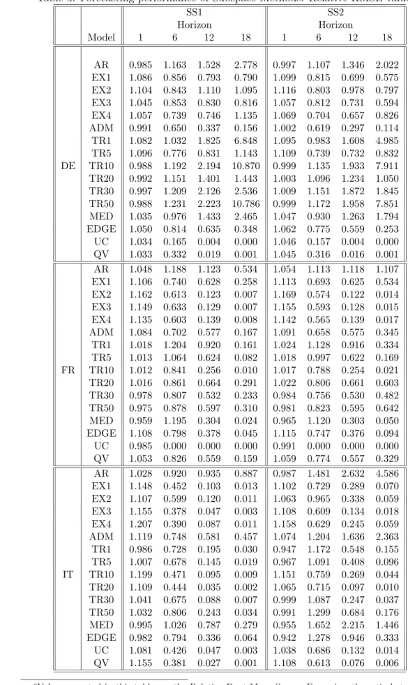
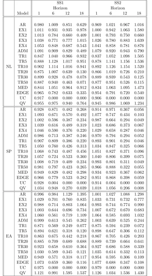
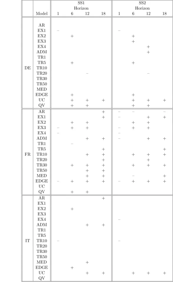
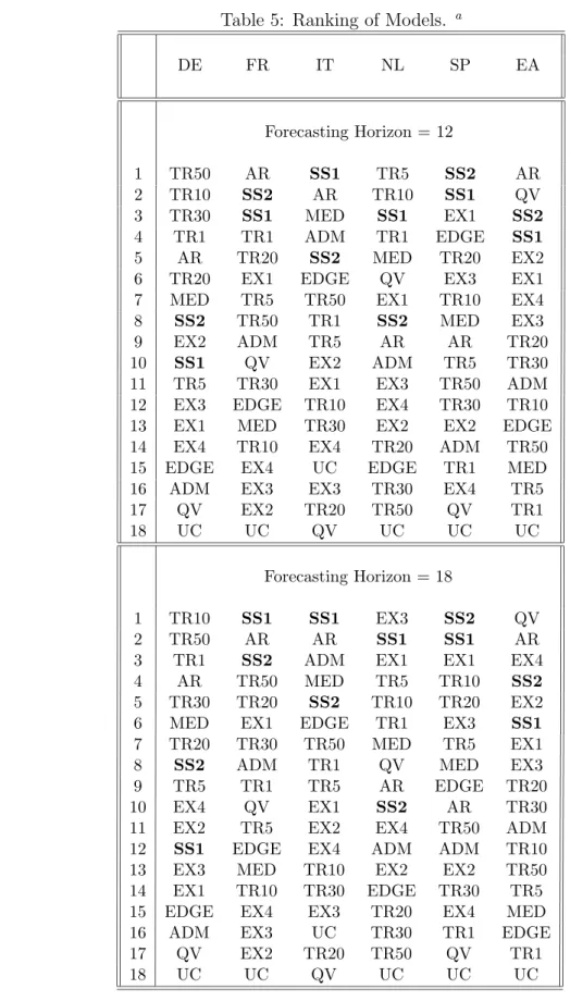
Tables 3 reports the forecasting performance of the dynamic factor meth-ods against the traditional methmeth-ods. Table 3 shows the Relative Root Mean Square Forecasting Error (RMSE) of the traditional method against the SS1 and SS2 methods. Diebold and Mariano (1995) tests of forecasting accuracy are provided in table 4. Finally, table 5 ranks all methods from best to worst according to their accuracy at forecasting inflation over a 12 and 18 month horizon.

With the exception of Germany, the dynamic factor methods provide always either the best or close to best performance. Those methods that perform best for Germany display a rather bad performance in France, Italy, the Netherlands, Spain and the euro area. This is not the case for the sub-space method SS1, which does not have a very low ranking for Germany either. The performance of the SS1 method is always very good with the exception of Germany.

5

Conclusion

This paper has explored the forecasting ability of core inflation measures built using dynamic factor methods against those built using more traditional techniques. Dynamic factor methods allow both the cross section dimension and the times series dimension of the data to be exploited in building a core inflation measure. These methods are applicable to large datasets. The

measures of core inflation built by means of dynamic factor methods are found to perform well in comparison to traditional measures in terms of their forecasting performance. This paper has also warned that measures of underlying inflation based on methods that ignore the time series dimension may fail to cointegrate with headline inflation.

References

Bauer, D. (1998): “Some Asymptotic Theory for the Estimation of Linear Systems Using Maximum Likelihood Methods or Subspace Algorithms,” Institute f. Econometrics, Operation Research and System Theory, TU Wien, Austria, PhD Thesis.

Blanchard, O. J., and D. Quah (1989): “The Dynamic Effects of Ag-gregate Demand and Supply Disturbances,” _{American Economic Review}, 79, 655–673.

Blinder, A. S. (1997): “Comment,” Federal Reserve Bank of St Louis

Review, 79(May/June), 157–160.

Bryan, M. F., and S. G. Cecchetti(1993): “The Consumer Price Index as a measure of Inflation,” _{Federal Reserve Bank of Cleveland Economic}

Review, pp. 15–24.

(1994): “Measuring Core Inflation,” in _{Monetary Policy}, ed. by N. G. Mankiw. Chicago University Press.

Diebold, F. X., and R. S. Mariano (1995): “Comparing Predictive Accuracy,” _{Journal of Business and Economic Statistics}, 13, 253–263. ECB(2004): “The impact of Developments in Direct taxes and administered

prices on inflation,” European Central Bank Monthly Bulletin, January, 2004.

Hannan, E. J., andM. Deistler(1988): The Statistical Theory of Linear

Systems. John Wiley.

Harvey, A. C. (1993): Time Series Models. Harvester and Wheatsheaf. Harvey, A. C., and A. Jaeger (1993): “Detrending, stylized facts and

Johansen, S.(1988): “Statistical analysis of cointegration vectors,”Journal

of Economic Dynamics and Control, 12, 231–254.

Kapetanios, G. (2004): “A Note on modelling Core inflation for the UK using a new dynamic factor estimation method and a large disaggregated price index dataset,”_{Economics Letters}, 85, 63–69.

Kapetanios, G., and M. Marcellino(2003): “A Parametric Estimation Method for Dynamic Factor Models of Large Dimensions,” Queen Mary, University of London Working Paper No 489, April 2003.

Larimore, W. E. (1983): “System Identification, Reduced Order Filters and Modeling via Canonical Variate Analysis,” in_{Proc. 1983 Amer.}

Con-trol Conference 2, ed. by H. S. Rao,and P. Dorato. Piscataway, NJ. IEEE Service Center.

L¨utkepohl, H. (1991): Introduction to Multiple Time Series Analysis. Springer, Berlin.

Magnus, J. R., and H. Neudecker(1988): Matrix Differential Calculus

with applications in Statistics and Econometrics. John Wiley and Sons. Overschee, P. V., and B. D. Moor (1996): Subspace Identification for

LInear Systems. Kluwer Academic Publishers.

Perron, P. (1989): “The great crash, the oil price shock and the unit root hypothesis,” _Econometrica, 57(6), 1361–1401.

Quah, D., andS. P. Vahey(1995): “Measuring Core Inflation,”Economic

Journal, 105, 1130–1140.

Solans, E. D. (2001): “Issues concerning the use and measure-ment of the Harmonised Index of Consumer Prices (HICP),” speech delivered at the CEPR/ECB Workshop on issues in the measure-ment of price indices, Frankfurt am Main, 16 November 2001. http://www.ecb.int/key/01/sp011116.htm.

Stock, J. H., and M. W. Watson (2002): “Macroeconomic forecast-ing usforecast-ing diffusion indices,” _{Journal of Business and Economic Statistics}, 20(2), 147–162.

Vega, J. L., and M. A. Wynne(2001): “An evaluation of some measures of core inflation for the euro area,” European Central Bank Working Paper No 53, April.

Wynne, M. A. (1999): “Core Inflation: A review of some conceptual is-sues,” European Central Bank, Working Paper No 5, May 1999.

Table 1: Unit root test.a DE FR IT NL SP EA HICP τ -0.33 0.52 -2.68 -0.86 -0.64 -0.51 τµ -2.64 -0.75 -4.71 -2.18 -2.60 -1.46 EX1 τ -0.66 0.25 -1.04 -0.97 -0.65 -0.69 τµ -2.43 -0.80 -3.08 -1.85 -2.06 -1.55 EX2 τ -0.67 -0.13 -1.30 -0.52 -0.80 -0.51 τµ -2.53 -1.37 -3.11 -1.75 -2.72 -2.41 EX3 τ -0.49 1.07 -1.15 -0.73 -0.74 -0.29 τµ -2.25 0.09 -3.12 -1.64 -2.71 -2.14 EX4 τ -0.45 0.76 -1.10 -0.84 -0.81 -0.27 τµ -2.55 -0.38 -3.16 -1.78 -2.12 -2.06 ADM τ -0.37 0.14 -0.95 -0.36 -0.83 -0.37 τµ -1.79 -1.28 -2.74 -2.12 -2.85 -2.36 TR1 τ -0.66 0.35 -0.86 -0.74 -0.68 -0.59 τµ -2.47 -0.93 -2.56 -1.91 -2.52 -1.46 TR5 τ -0.65 0.27 -0.87 -0.75 -0.64 -0.29 τµ -1.98 -0.97 -2.65 -1.85 -2.55 -1.32 TR10 τ -0.75 0.10 -0.83 -0.76 -0.54 -0.40 τµ -1.97 -1.38 -2.64 -1.44 -2.38 -1.63 TR20 τ -0.92 0.01 -0.76 -0.84 -0.56 -0.51 τµ -2.05 -1.14 -2.63 -1.56 -1.83 -1.93 TR30 τ -0.97 0.09 -0.72 -0.82 -0.59 -0.48 τµ -2.10 -1.09 -2.64 -1.56 -1.81 -1.94 TR50 τ -0.86 0.15 -0.70 -0.59 -0.50 -0.72 τµ -2.11 -0.98 -2.83 -1.62 -1.63 -1.76 MED τ -1.17 0.68 -1.23 -0.47 -0.47 -0.99 τµ -1.97 -1.56 -3.75 -1.79 -1.26 -1.94 EDGE τ -1.60 -0.05 -1.04 -0.76 -0.94 -1.46 τµ -2.09 -0.75 -2.83 -1.00 -2.32 -1.83 UC τ -0.31 0.20 -2.26 -0.86 -0.77 -0.47 τµ -2.44 -1.44 -4.39 -2.33 -2.26 -1.65 QV τ -1.23 0.41 -3.68 -1.47 -0.26 -0.73 τµ -1.93 -0.70 -4.24 -2.74 -2.22 -1.60 SS1 τ -2.90 -1.63 -2.56 -1.62 -1.23 -2.34 τµ -2.87 -1.63 -2.88 -1.60 -1.19 -2.32 SS2 τ -1.14 -0.45 -0.92 -1.57 -0.31 0.00 τµ -1.25 -2.09 -5.34 -3.60 -2.39 -1.58

a_{This tables presents the Augmented Dickey-Fuller statistics computed without and interceptτ and with}

and interceptτ_µ. The 5% critical values are -1.95 and -2.86 respectively. The criterium followed to determine the number of lags is that suggested by Perron (1989); namely choose a lag length such that the t-statistics

Table 2: Cointegration and Exogenity Tests.a DE FR IT NL SP EA EX1 Coint. - - - -Exogen. 0.046∗∗ 0.854 0.445 0.050∗∗ 0.110 0.880 EX2 Coint. - - - √ - -Exogen. 0.002∗∗ 0.159 0.014∗∗ 0.077∗ 0.046∗∗ 0.320 EX3 Coint. - - - √ - -Exogen. 0.013∗∗ 0.165 0.671 0.077∗ 0.088∗ 0.574 EX4 Coint. - - - √ - -Exogen. 0.036∗∗ 0.281 0.368 0.067∗ 0.048∗∗ 0.719 ADM Coint. - - - -Exogen. 0.006∗∗ 0.626 0.241 0.007∗∗ 0.069∗ 0.697 TR1 Coint. - - - - √ -Exogen. 0.186 0.552 0.999 0.569 0.465 0.127 TR5 Coint. - - - -Exogen. 0.919 0.459 0.834 0.023∗∗ 0.758 0.195 TR10 Coint. - - - -Exogen. 0.938 0.336 0.853 0.107 0.268 0.161 TR20 Coint. - - - -Exogen. 0.869 0.275 0.931 0.557 0.022∗∗ 0.299 TR30 Coint. - - - -Exogen. 0.694 0.193 0.660 0.637 0.011∗∗ 0.130 TR50 Coint. - - √ - - -Exogen. 0.611 0.093∗ 0.153 0.806 0.013∗∗ 0.109 MED Coint. - - √ - - -Exogen. 0.526 0.098∗ 0.212 0.859 0.082∗ 0.185 EDGE Coint. - - - -Exogen. 0.901 0.115 0.379 0.557 0.234 0.914 UC Coint. √ √ √ √ √ √ Exogen. 0.162 0.007∗∗ 0.040∗∗ 0.107 0.990 0.008∗∗ QV Coint. - - √ - - -Exogen. 0.344 0.193 0.000∗∗ 0.079∗ 0.006∗∗ 0.018∗∗ SS1 Coint. - - - -Exogen. 0.140 0.396 0.000∗∗ 0.025∗∗ 0.619 0.702 SS2 Coint. - - - - √ -Exogen. 0.000∗∗ 0.874 0.111 0.101 0.001∗∗ 0.018∗∗

a_{The cointegration test conducted is that of Johansen (1988). The exogeneity}

test is conducted along the lines explained in L¨utkepohl (1991, ch. 11), values reported are probability values.

Table 3: Forecasting performance of Subspace Methods. Relative RMSE values.a SS1 SS2 Horizon Horizon Model 1 6 12 18 1 6 12 18 AR 0.985 1.163 1.528 2.778 0.997 1.107 1.346 2.022 EX1 1.086 0.856 0.793 0.790 1.099 0.815 0.699 0.575 EX2 1.104 0.843 1.110 1.095 1.116 0.803 0.978 0.797 EX3 1.045 0.853 0.830 0.816 1.057 0.812 0.731 0.594 EX4 1.057 0.739 0.746 1.135 1.069 0.704 0.657 0.826 ADM 0.991 0.650 0.337 0.156 1.002 0.619 0.297 0.114 TR1 1.082 1.032 1.825 6.848 1.095 0.983 1.608 4.985 TR5 1.096 0.776 0.831 1.143 1.109 0.739 0.732 0.832 DE TR10 0.988 1.192 2.194 10.870 0.999 1.135 1.933 7.911 TR20 0.992 1.151 1.401 1.443 1.003 1.096 1.234 1.050 TR30 0.997 1.209 2.126 2.536 1.009 1.151 1.872 1.845 TR50 0.988 1.231 2.223 10.786 0.999 1.172 1.958 7.851 MED 1.035 0.976 1.433 2.465 1.047 0.930 1.263 1.794 EDGE 1.050 0.814 0.635 0.348 1.062 0.775 0.559 0.253 UC 1.034 0.165 0.004 0.000 1.046 0.157 0.004 0.000 QV 1.033 0.332 0.019 0.001 1.045 0.316 0.016 0.001 AR 1.048 1.188 1.123 0.534 1.054 1.113 1.118 1.107 EX1 1.106 0.740 0.628 0.258 1.113 0.693 0.625 0.534 EX2 1.162 0.613 0.123 0.007 1.169 0.574 0.122 0.014 EX3 1.149 0.633 0.129 0.007 1.155 0.593 0.128 0.015 EX4 1.135 0.603 0.139 0.008 1.142 0.565 0.139 0.017 ADM 1.084 0.702 0.577 0.167 1.091 0.658 0.575 0.345 TR1 1.018 1.204 0.920 0.161 1.024 1.128 0.916 0.334 TR5 1.013 1.064 0.624 0.082 1.018 0.997 0.622 0.169 FR TR10 1.012 0.841 0.256 0.010 1.017 0.788 0.254 0.021 TR20 1.016 0.861 0.664 0.291 1.022 0.806 0.661 0.603 TR30 0.978 0.807 0.532 0.233 0.984 0.756 0.530 0.482 TR50 0.975 0.878 0.597 0.310 0.981 0.823 0.595 0.642 MED 0.959 1.195 0.304 0.024 0.965 1.120 0.303 0.050 EDGE 1.108 0.798 0.378 0.045 1.115 0.747 0.376 0.094 UC 0.985 0.000 0.000 0.000 0.991 0.000 0.000 0.000 QV 1.053 0.826 0.559 0.159 1.059 0.774 0.557 0.329 AR 1.028 0.920 0.935 0.887 0.987 1.481 2.632 4.586 EX1 1.148 0.452 0.103 0.013 1.102 0.729 0.289 0.070 EX2 1.107 0.599 0.120 0.011 1.063 0.965 0.338 0.059 EX3 1.155 0.378 0.047 0.003 1.108 0.609 0.134 0.018 EX4 1.207 0.390 0.087 0.011 1.158 0.629 0.245 0.059 ADM 1.119 0.748 0.581 0.457 1.074 1.204 1.636 2.363 TR1 0.986 0.728 0.195 0.030 0.947 1.172 0.548 0.155 TR5 1.007 0.678 0.145 0.019 0.967 1.091 0.408 0.096 IT TR10 1.199 0.471 0.095 0.009 1.151 0.759 0.269 0.044 TR20 1.109 0.444 0.035 0.002 1.065 0.715 0.097 0.010 TR30 1.041 0.675 0.088 0.007 0.999 1.087 0.247 0.037 TR50 1.032 0.806 0.243 0.034 0.991 1.299 0.684 0.176 MED 0.995 1.026 0.787 0.279 0.955 1.652 2.215 1.446 EDGE 0.982 0.794 0.336 0.064 0.942 1.278 0.946 0.333

Table 3 (cont): Forecasting performance of Subspace Methods. Relative RMSE values.a SS1 SS2 Horizon Horizon Model 1 6 12 18 1 6 12 18 AR 0.980 1.009 0.851 0.629 0.969 1.021 0.967 1.016 EX1 1.011 0.931 0.935 0.978 1.000 0.942 1.063 1.580 EX2 1.013 0.784 0.660 0.409 1.001 0.793 0.750 0.660 EX3 1.038 0.771 0.777 1.015 1.026 0.780 0.883 1.639 EX4 1.053 0.848 0.687 0.543 1.041 0.858 0.781 0.876 ADM 1.091 0.909 0.829 0.489 1.079 0.920 0.943 0.790 TR1 0.847 1.040 0.966 0.932 0.837 1.052 1.098 1.505 TR5 0.888 1.128 1.017 0.951 0.878 1.141 1.156 1.536 NL TR10 0.902 1.114 1.016 0.941 0.892 1.126 1.154 1.520 TR20 0.875 1.007 0.639 0.130 0.866 1.019 0.726 0.210 TR30 0.899 0.928 0.478 0.078 0.889 0.939 0.543 0.125 TR50 0.887 0.940 0.463 0.071 0.877 0.951 0.526 0.115 MED 0.844 1.051 0.964 0.912 0.834 1.063 1.095 1.473 EDGE 0.965 0.782 0.633 0.335 0.954 0.791 0.720 0.540 UC 0.917 0.000 0.000 0.000 0.906 0.000 0.000 0.000 QV 0.955 0.975 0.940 0.764 0.945 0.986 1.069 1.234 AR 0.928 0.871 0.482 0.268 0.914 0.971 0.367 0.056 EX1 1.093 0.671 0.570 0.492 1.077 0.747 0.434 0.103 EX2 1.002 0.596 0.387 0.234 0.987 0.664 0.294 0.049 EX3 1.039 0.616 0.489 0.319 1.023 0.686 0.373 0.067 EX4 1.046 0.590 0.376 0.220 1.029 0.658 0.287 0.046 ADM 0.986 0.713 0.387 0.246 0.970 0.794 0.294 0.052 TR1 0.907 0.809 0.386 0.220 0.893 0.901 0.294 0.046 TR5 1.050 0.760 0.426 0.313 1.034 0.847 0.325 0.066 SP TR10 1.068 0.743 0.487 0.456 1.051 0.827 0.371 0.096 TR20 1.057 0.724 0.523 0.360 1.040 0.806 0.399 0.075 TR30 1.008 0.719 0.409 0.234 0.993 0.801 0.311 0.049 TR50 0.981 0.797 0.423 0.265 0.966 0.888 0.322 0.055 MED 0.949 0.829 0.482 0.298 0.934 0.923 0.367 0.062 EDGE 0.966 0.779 0.523 0.282 0.951 0.868 0.398 0.059 UC 0.928 0.004 0.000 0.000 0.914 0.004 0.000 0.000 QV 1.034 0.948 0.270 0.039 1.018 1.056 0.206 0.008 AR 0.996 0.984 1.129 1.395 1.001 1.027 1.088 1.298 EX1 1.029 0.701 0.760 0.835 1.033 0.731 0.732 0.777 EX2 0.988 0.714 0.803 1.064 0.993 0.744 0.774 0.990 EX3 1.003 0.644 0.696 0.734 1.007 0.672 0.670 0.683 EX4 1.060 0.561 0.719 1.109 1.064 0.585 0.693 1.032 ADM 0.999 0.613 0.545 0.262 1.003 0.639 0.525 0.244 TR1 0.871 0.569 0.249 0.077 0.875 0.594 0.239 0.072 TR5 0.894 0.621 0.318 0.120 0.898 0.647 0.306 0.112 EA TR10 0.863 0.675 0.442 0.218 0.867 0.705 0.426 0.203 TR20 0.885 0.709 0.689 0.688 0.889 0.739 0.664 0.641 TR30 0.923 0.658 0.610 0.364 0.927 0.686 0.588 0.339 TR50 1.030 0.589 0.345 0.121 1.035 0.614 0.332 0.113 MED 0.949 0.571 0.318 0.117 0.954 0.595 0.306 0.109 EDGE 1.073 0.659 0.360 0.116 1.077 0.688 0.347 0.108

Table 4: Forecasting performance of Subspace Methods. Diebold-Mariano tests.a SS1 SS2 Horizon Horizon Model 1 6 12 18 1 6 12 18 AR EX1 – – EX2 + + EX3 + EX4 + ADM + TR1 TR5 + + DE TR10 TR20 – – TR30 TR50 MED EDGE + + UC + + + + + + QV + + + + AR + – – – EX1 + – + + EX2 + + + + EX3 – + + – + + EX4 – – ADM + + – + + TR1 – TR5 + + FR TR10 + + + + + TR20 + + TR30 + + + + + + TR50 + + MED + + – + EDGE – + + + – + + + UC QV + + AR + EX1 EX2 + EX3 EX4 – ADM + + TR1 TR5 IT TR10 – – TR20 TR30 TR50 MED + EDGE +

Table 4 (cont): Forecasting performance of Subspace Methods. Diebold-Mariano tests.a SS1 SS2 Horizon Horizon Model 1 6 12 18 1 6 12 18 AR EX1 EX2 + + EX3 EX4 + + + ADM + TR1 TR5 – NL TR10 TR20 + + + TR30 + + + + TR50 + MED EDGE + + UC QV AR + EX1 + + + + + EX2 + + + + EX3 + EX4 ADM + + + + TR1 + + + + TR5 + SP TR10 + + + + TR20 + + + + TR30 + + + TR50 + + + + MED EDGE + + UC + + QV AR – – EX1 + + EX2 + EX3 + + EX4 + + ADM + + TR1 + + + + TR5 + + EA TR10 + + + + + + TR20 + TR30 + TR50 + + + + MED + + EDGE + + – + + UC + +

Table 5: Ranking of Models. a DE FR IT NL SP EA Forecasting Horizon = 12 1 TR50 AR SS1 TR5 SS2 AR 2 TR10 SS2 AR TR10 SS1 QV 3 TR30 SS1 MED SS1 EX1 SS2 4 TR1 TR1 ADM TR1 EDGE SS1 5 AR TR20 SS2 MED TR20 EX2

6 TR20 EX1 EDGE QV EX3 EX1

7 MED TR5 TR50 EX1 TR10 EX4

8 SS2 TR50 TR1 SS2 MED EX3

9 EX2 ADM TR5 AR AR TR20

10 SS1 QV EX2 ADM TR5 TR30

11 TR5 TR30 EX1 EX3 TR50 ADM

12 EX3 EDGE TR10 EX4 TR30 TR10

13 EX1 MED TR30 EX2 EX2 EDGE

14 EX4 TR10 EX4 TR20 ADM TR50

15 EDGE EX4 UC EDGE TR1 MED

16 ADM EX3 EX3 TR30 EX4 TR5

17 QV EX2 TR20 TR50 QV TR1

18 UC UC QV UC UC UC

Forecasting Horizon = 18

1 TR10 SS1 SS1 EX3 SS2 QV

2 TR50 AR AR SS1 SS1 AR

3 TR1 SS2 ADM EX1 EX1 EX4

4 AR TR50 MED TR5 TR10 SS2

5 TR30 TR20 SS2 TR10 TR20 EX2

6 MED EX1 EDGE TR1 EX3 SS1

7 TR20 TR30 TR50 MED TR5 EX1

8 SS2 ADM TR1 QV MED EX3

9 TR5 TR1 TR5 AR EDGE TR20

10 EX4 QV EX1 SS2 AR TR30

11 EX2 TR5 EX2 EX4 TR50 ADM

12 SS1 EDGE EX4 ADM ADM TR10

13 EX3 MED TR10 EX2 EX2 TR50

14 EX1 TR10 TR30 EDGE TR30 TR5

15 EDGE EX4 EX3 TR20 EX4 MED

16 ADM EX3 UC TR30 TR1 EDGE

17 QV EX2 TR20 TR50 QV TR1

Figure 1: Harmonised index of Consumer Prices. Year on Year changes (%).

0

1

2

3

4

5

6

Jan-96

Jan-97

Jan-98

Jan-99

Jan-00

Jan-01

Jan-02

Jan-03

Jan-04

Figure 2: Harmonised index of Consumer Prices. Year on Year changes (%).

0

1

2

3

4

5

6

Jan-96

Jan-97

Jan-98

Jan-99

Jan-00

Jan-01

Jan-02

Jan-03

Jan-04

European Central Bank working paper series

For a complete list of Working Papers published by the ECB, please visit the ECB’s website (http://www.ecb.int)

380 “Optimal monetary policy under discretion with a zero bound on nominal interest rates” by K. Adam and R. M. Billi, August 2004.

381 “Fiscal rules and sustainability of public finances in an endogenous growth model” by B. Annicchiarico and N. Giammarioli, August 2004.

382 “Longer-term effects of monetary growth on real and nominal variables, major industrial countries, 1880-2001” by A. A. Haug and W. G. Dewald, August 2004.

383 “Explicit inflation objectives and macroeconomic outcomes” by A. T. Levin, F. M. Natalucci and J. M. Piger, August 2004.

384 “Price rigidity. Evidence from the French CPI micro-data” by L. Baudry, H. Le Bihan, P. Sevestre and S. Tarrieu, August 2004.

385 “Euro area sovereign yield dynamics: the role of order imbalance” by A. J. Menkveld, Y. C. Cheung and F. de Jong, August 2004.

386 “Intergenerational altruism and neoclassical growth models” by P. Michel, E. Thibault and J.-P. Vidal, August 2004.

387 “Horizontal and vertical integration in securities trading and settlement” by J. Tapking and J. Yang, August 2004.

388 “Euro area inflation differentials” by I. Angeloni and M. Ehrmann, September 2004. 389 “Forecasting with a Bayesian DSGE model: an application to the euro area” by F. Smets

and R. Wouters, September 2004.

390 “Financial markets’ behavior around episodes of large changes in the fiscal stance” by S. Ardagna, September 2004.

391 “Comparing shocks and frictions in US and euro area business cycles: a Bayesian DSGE approach” by F. Smets and R. Wouters, September 2004.

392 “The role of central bank capital revisited” by U. Bindseil, A. Manzanares and B. Weller, September 2004.

393 ”The determinants of the overnight interest rate in the euro are” by J. Moschitz, September 2004.

396 “The short-term impact of government budgets on prices: evidence from macroeconomic models” by J. Henry, P. Hernández de Cos and S. Momigliano, October 2004.

397 “Determinants of euro term structure of credit spreads” by A. Van Landschoot, October 2004. 398 “Mergers and acquisitions and bank performance in Europe: the role of strategic similarities” 399 “Sporadic manipulation in money markets with central bank standing facilities”

by C. Ewerhart, N. Cassola, S. Ejerskov and N. Valla, October 2004.

400 “Cross-country differences in monetary policy transmission” by R.-P. Berben, A. Locarno, J. Morgan and J. Valles, October 2004.

401 “Foreign direct investment and international business cycle comovement” by W. J. Jansen and A. C. J. Stokman, October 2004.

402 “Forecasting euro area inflation using dynamic factor measures of underlying inflation” ndez and G. Kapetanios, November 2004.

by Y. Altunbas and D. Marqués Ibáñez, October 2004.

é by G. Camba-M