on Topology Analysis
Gunther H. Weber1,2 and Gerik Scheuermann1 1
AG Graphische Datenverarbeitung und Computergeometrie, FB Informatik, University of Kaiserslautern, Germany,{weber,scheuer}@informatik.uni-kl.de 2
Center for Image Processing and Integrated Computing, Dept. of Computer Science, University of California, Davis, U.S.A., [email protected]
Summary. Direct Volume Rendering (DVR) is commonly used to visualize scalar fields. Quality and significance of rendered images depend on the choice of appro-priate transfer functions that assigns optical properties (e.g., color and opacity) to scalar values. We present a method that automatically generates a transfer func-tion based on the topological behavior of a scalar field. Given a scalar field defined by piecewise trilinear interpolation over a rectilinear grid, we find a set of critical isovalues for which the topology of an isosurface, i.e., a surface representing all lo-cations where the scalar field assumes a certain valuev, changes. We then generate a transfer function that emphasizes on scalar values around those critical isoval-ues. Images rendered using the resulting transfer function reveal the fundamental topological structure of a scalar data set.
1 Introduction
Direct Volume Rendering visualizes a three-dimensional (3D) scalar field by using a transfer function to map scalar values to optical properties (e.g., color and opacity) and rendering the resulting image. This transfer function presents a user with an additional parameter that influences a resulting vi-sualization. However, quality and significance of the resulting visualization hinge on a sensible choice of the transfer function. Transfer functions are commonly determined manually by trial and error which is time-consuming and prone to errors. Several attempts were made to analyze a data set and generate appropriate transfer functions automatically to aid a user in the vi-sualization process. Pfister et al. [11] give an overview over several techniques and compare results with manually chosen transfer functions.
Apart from DVR, isosurfaces are most commonly used to visualize scalar fields f(x, y, z). An isosurface represents all locations in 3D space, where f assumes a given isovalue v, i.e., where f =v holds. By varying the isovalue v, it is possible to visualize the entire scalar field. Like choosing appropriate transfer functions, determining isovalues where “interesting” isosurface be-havior occurs is difficult. Weber et al. [12] have considered the topological properties of scalar fields defined by piecewise trilinear interpolation used on
rectilinear grids to determine for which isovalues relevant isosurface behav-ior occurs. All fundamental changes are tracked: Closed surface components emerge or vanish at local minima or maxima, and thegenusof an isosurface changes, i.e., holes appear/disappear in a surface component, or disjoint sur-face components merge at saddles. Values and locations where such changes occur are determined and used to aid a user in data exploration.
Instead of using the resulting set of critical isovalues as indicator for which isovalues expressive isosurfaces result, it is possible to use them to construct a transfer function that highlights topological properties of a scalar data set. DVR commonly uses trilinear interpolation within cells. Thus, critical isovalues extracted by Weber et al. [12] are also meaningful in a volume rendering context. We use the resulting list of critical isovalues to design transfer functions based on the work presented by Fujishiro et al. [5, 7]. We generate transfer functions that assign small opacity to all scalar values except those close to critical isovalues. Colors are assigned using an HLS color model and varying the hue component for different scalar values such that it changes more rapidly close to critical isovalues.
2 Related Work
Few authors utilize topological analysis for scalar field visualization. Bajaj et al. [1] determined acontour spectrumfor data given on tetrahedral meshes. The contour spectrum specifies contour properties like 2D contour length, 3D contour area and gradient integral as functions of the isovalue and can aid a user in identifying “interesting” isovalues. Bajaj et al. [3] also devel-oped a technique to visualize topology to enhance visualizations of trivariate scalar fields. Their method employs a C1-continuous interpolation scheme for rectilinear grids, and detects critical points of a scalar field, i.e., points where the gradient of the scalar field vanishes. Subsequently, integral curves (tangent curves) are traced starting from locations close to saddle points. These integral curves are superimposed onto volume-rendered images to con-vey structural information of the scalar field.
Fujishiro et al. [5] used ahyper-Reeb graphfor exploration of scalar fields. A Reeb graph encodes topology of a surface. The hyper-Reeb graph encodes changes of topology in an extracted isosurface. For each isovalue that cor-responds to an isosurface topology change, a node exists in the hyper-Reeb graph containing a Reeb graph encoding the topology of that isosurface. Fu-jishiro et al. [5] constructed a hyper-Reeb graph using “focusing with interval volumes,” an iterative approach that finds a subset of all critical isovalues , which has been introduced by Fujishiro and Takeshima [6]. The hyper-Reeb graph can be used, for example, for automatic generation of transfer func-tions. Fujishiro et al. [7] extended this work and used a hyper-Reeb graph for exploration of volume data. In addition to automatic transfer function de-sign, their extended method allows them to generate translucent isosurfaces
between critical isovalues. Considering just the images shown in their paper, it seems that their approach does not detect all critical isovalues of a scalar field.
Critical point behavior is also important in the context of data simplifi-cation to preserve important features of a data set. Bajaj and Schikore [2] extended previous methods to develop a compression scheme preserving topo-logical features. Their approach detects critical points of a piecewise linear bivariate scalar field f(x, y). “Critical vertices” are those vertices for which the “normal space” of the surrounding triangle platelet contains the vector (0,0,1). Integral curves are computed by tracing edges of triangles along a “ridge” or “channel.” Bajaj and Schikore’s method incorporates an error measure and can be used for topology-preserving mesh simplification.
Gerstner and Pajarola [8] defined a bisection scheme that enumerates all grid points of a rectilinear grid in a tetrahedral hierarchy. Using piecewise linear interpolation in tetrahedra, critical points can be detected. Data sets are simplified by specifying a traversal scheme that descends only as deep into the tetrahedral hierarchy as necessary to preserve topology within a cer-tain error bound. This method incorporates heuristics that assign importance values to topological features, enabling a controlled topology simplification.
3 Detecting Critical Isovalues
Our goal is to detectcritical isovaluesof a piecewise trilinear scalar field given on a regular rectilinear grid. Gerstner and Pajarola [8] developed criteria for detecting critical points of piecewise linear scalar fields defined on tetrahedral meshes and used them in mesh simplification. We provide a comprehensive analysis of the topological behavior of piecewise trilinear interpolation and develop criteria to detect critical isovalues for these scalar fields. We further develop methods to use these critical isovalues for volume data exploration.
3.1 Definitions
For aC2-continuous functionf, critical points occur where the gradient∇f assumes a value of zero, i.e., ∇f = 0. The type of a critical point can be determined by the signs of the eigenvalues of the Hermitian off. Piecewise trilinear interpolation when applied to rectilinear grids, in general, produces only C0-continuous functions. Therefore, we must define critical points dif-ferently.
Gerstner and Pajarola [8] considered piecewise linear interpolation applied to tetrahedral grids, which also leads toC0-continuous functions. Considering piecewise linear interpolation, critical points can only occur at mesh vertices. Gerstner and Pajarola’s method classifies a mesh vertex depending on its relationship with vertices in a local neighborhood. In the context of a refine-ment scheme, all tetrahedra sharing an edge that is to be collapsed define
a “surrounding polyhedron.” Vertices of this surrounding polyhedron con-stitute the considered neighborhood of a vertex. These vertices are marked with a “+” if their associated function values are greater than the value of the classified vertex; or they are marked with a “-” if their associated function values are less than the value of the classified vertex. Equal values are not considered. Edges of the surrounding polyhedron define an edge graph. In this graph, all edges connecting vertices of different polarities are deleted. A vertex is classified according to the number of connected components in the remaining graph. If this number is one, the classified vertex is a maximum or minimum (depending on the sign of the connected component). If it is two, the classified vertex is a regular point. Otherwise, the vertex is a saddle point. Connected components in an edge graph of a surrounding polyhedron correspond to connected components in a neighborhood of a vertex. This observation leads us to the following definition:
Definition 1 (Regular and Critical Points). Let F : Rd →
R, d ≥ 2, be a continuous function. A point x ∈ Rd is called a (a) regular point, (b) minimum, (c) maximum, (d) saddle, or (e) flat point of F, if for all >0 there exists a neighborhoodU ⊂Uwith the following properties: IfS˙
np
i=1Pi is a partition of the preimage of[F(s),+∞)inU−{x}into “positive” connected components andS˙nn
j=jNj is a partition of the preimage of(−∞, F(s))]inU−
{x} into “negative” connected components, then (a) np =nn = 1 andP1 6= N1, (b)np = 1 andnn= 0, (c)nn = 1 andnp= 0, (d) np+nn >2, or (e) np=nn= 1 andP1=N1.
(a) (b) (c) (d)
Fig. 1.(a) Around a regular pointx∈R3, the isosurfaceF−1(F(x)) divides space into a single connected volumeP withF >0 (dark gray) and a single connected volumeNwithF <0 (white). (b) Around a minimum, all points inUhave a larger value thanF(x). (c) Around a maximum, every point inU has a smaller value than
F(x). (d) In case of a saddle, there are more than one separated regions with values larger or smaller than the valueF(x)
Remark 1.For (a) – (d), see Fig. 1. Concerning case (e), all points inU have the same value asF(x). It is possible to extend the concept of being critical to entire regions and classify regions rather than specific locations.
Remark 2.The casesnp= 2, nn = 0 andnp= 0,nn= 2 are not possible for d≥2.
We consider piecewise trilinear interpolation, which reduces to bilinear interpolation on cell faces and to linear interpolation along cell edges. All values that trilinear interpolation assigns to positions in a cell lie between the minimal and maximal function values at the cell’s vertices (convex hull property). In fact, maxima and minima can only occur at cell vertices. If two vertices connected by an edge have the same function value, the entire edge can represent an extremum or a saddle. It is even possible that a polyline defined by multiple edges in the grid, or a region consisting of several cells, becomes critical. In these cases, it is no longer possible to determine, locally, whether a function value is a critical isovalue. To avoid these types of prob-lem, we impose the restriction on the data that function values at vertices connected by an edge must differ. Saddles can occur at cell vertices, on cell faces of a cell, and in a cell’s interior, but not on cell edges. This fact is due to the restriction that an edge cannot have one constant function value. Lemma 1 (Regular Edge Points). All points on edges of a trilinear in-terpolant with distinct edge-connected values are regular points.
Proof. By assumption, the two endpoints of the edge have different values. Interpolation along edges is linear, and the derivative differs from zero. The implicit function theorem defines neighborhoodsUi×Viand a height function hi:Ui ⇒Viin each of the four cubes around the edge, such that the isosurface is a height field in the direction of the edge. SettingU to the smallest interval and determining suitableUi defines a neighborhood such that the larger and smaller values are above and below a single height field. Therefore, a point on an edge is a regular point, because it is possible to start the construction
with an arbitrary small neighborhood aroundx. ut
Thus, in order to detect critical isovalues of a piecewise trilinear scalar field, we only need to detect critical values at vertices of a grid and saddle values within cells and on their boundary faces.
3.2 Critical Values at Vertices
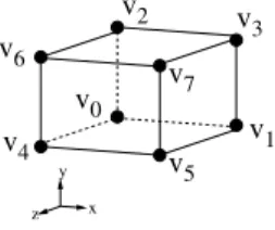
v0 v7 v5 v4 v6 v2 v 3 v1 y z x
In order to classify a vertex, i.e., to determine whether a vertex is regular or represents an extremum or a saddle, it is sufficient to consider the values at the six edge-connected vertices of a given vertex. We provide a criterion for classification in the following.
Lemma 2 (Local Maximum).Consider a cellCwith vertex numbering as shown in Fig. 2. If v0>max{v1, v2, v4}, thenv0 is a local maximum inC. Proof. Choosem:= max{v1−v0, v2−v0, v4−v0}<0 andM := max{v3− v0, v5−v0, v6−v0, v7−v0,1} ≥1. Letv0i=vi−v0. If 0< x, y, z < := | m| 3|M|, then F(x, y, z)−v0= (1−x)(1−y)(1−z)v00+x(1−y)(1−z)v01+ (1−x)y(1−z)v02+xy(1−z)v03+ (1−x)(1−y)zv04+x(1−y)zv05+ (1−x)yzv06+xyzv07 < x(1−y)(1−z)m+ (1−x)y(1−z)M+ xy(1−z)m+ (1−x)(1−y)zM+ x(1−y)zm+ (1−x)yzM+xyzM
≤m[(1−y)(1−z) + (1−x)(1−z) + (1−x)(1−y)] + M 2[1−z+ 1−x+z+ 1−y] ≤3m(1−)2+ 3M 2 = 3 |m| 3|M| sgn(m)|m| 1− |m| 3|M| 2 +M |m| 3|M| ! = |m| |M| −|m|+2 3 |m| |M|− |m|2 9|M|2 +M |m| 3|M| = |m| |M| −2 3|m|+ 2 3 |m| |M|− |m|2 9|M|2 ≤ |m| |M| −9|m| 2 |M|2 <0. ut
Lemma 3 (Linear Cell Partition).Consider a cellCwith vertex valuesvi and vertex positionspi numbered as shown in Fig. 2. Ifv:=v0=6 v1, v26=v4 holds, then for all >0 there exists a δ < such that for the intersection R = Uδ(p0)∩C the following statements hold: (a) If v > max{v1, v2, v4} thennn = 1and N1=R, i.e., all values in the region are less thanv. (b) If there existi, j, k∈ {1,2,4}, i6=j6=k, i6=k, such thatv >max{vi, vj} and v < vk, then nn =np = 1 andR completely contains a surface dividing N1 and P1. Furthermore, all values on the triangle p0pipj are less than v. (c) If there exist i, j, k ∈ {1,2,4}, i 6=j =6 k, i 6=k, such that v <min{vi, vj}
andv > vk, then nn=np= 1, andR completely contains a surface dividing N1 andP1. Furthermore, all values on the triangle p0pipj are less thanv. (d) If v <max{v1, v2, v4}, then nn = 1 andN1 =R, i.e., all values in the region are greater than v.
Proof. Cases (a) and (d) are symmetrical and follow from Lemma 2. Cases (b) and (c) are symmetrical as well, and it is sufficient to prove one of them. Similarly, the same holds when we choose any other vi asv and consider its edge-connected neighbor vertices.
Let >0. The derivative ofFatp0is (v1−v0, v2−v0, v4−v0). There exists an > δ >0 such that the derivative has rank 1 in the whole neighborhood R = Uδ(p0)∩C. In this case, the regular value theorem guarantees the existence of an isosurface with function valuev0dividingUδ(p0) into a single region with larger and a single region with lower function values. If the surface intersectsCoutsidep0,Ris split into exactly two parts. If not,p0 is a local
maximum or minimum. This fact proves the first part of (b) and (c). For small > δ >0, a calculation similar to the proof of Lemma 2 demonstrates that the face with p0,pi,pj is not intersected inside R by the isosurface in
cases (b) and (c). ut v (a) v (b) v (c) v (d)
Fig. 3.When a small neighborhood is considered, a “tetrahedral region” havingv
as a corner is partitioned in the same way as a linear tetrahedron
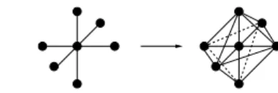
Using the L1-norm1, the intersection of a neighborhood with a cell cor-responds to a tetrahedron. According to Lemma 3, this tetrahedron is par-titioned in the same way as a tetrahedron using linear interpolation (even when, as in our case, partitioning surfaces are not necessarily planar), see Fig. 3. A vertex can be classified by considering its edge-connected neighbor vertices. We treat these vertices as part of a local implicit tetrahedrization surrounding a classified vertex, where the classified vertex and three edge-connected vertices belonging to the same rectilinear cell imply a tetrahedron, see Fig. 4.
When applying Gerstner and Pajarola’s criterion [8] for connected compo-nents in an edge graph for the resulting implicit tetrahedrization, we obtain
1 kxk1=P
Fig. 4.Edge-connected vertices as part of an implicit tetrahedrization
a case table with 26= 64 entries that maps a configuration of “+” and “-” of edge-connected vertices to a vertex classification. (It can be shown that the connected components in an edge graph correspond to connected components in a neighborhood.) We decided to generate this relatively small case table manually.
3.3 Critical Values on Faces
When linear interpolation is used, critical points can only occur at grid ver-tices. When piecewise trilinear interpolation is used, critical points can also occur on boundary faces. On a boundary face piecewise trilinear interpola-tion reduces to bilinear interpolainterpola-tion and the interpolant on a face can have a saddle. This face saddle is not necessarily a saddle of the piecewise trilin-ear interpolant. The following lemma provides a criterion to whether a face saddle is a saddle of the trilinear interpolant:
B−1 A1 D−1 D1 B1 A−1 C1 C−1 y z x A B D C
Fig. 5. Vertex numbering scheme used in Lemma 4
Lemma 4 (Face Saddle). Let pbe a point on the shared face of two cells, where both trilinear interpolants degenerate to the same bilinear interpolant. The point pis a saddle point when these two statements hold:
1. The point p is a saddle point of the bilinear interpolant defined on the face.
2. With the notations of Fig. 5, where, without loss of generality, cells are rotated such thatAandC are the values on the shared cell face having a value larger than the saddle value,C(A1−A) +A(C1−C)−D(B1−B)− B(D1−D)andC(A−1−A) +A(C−1−C)−D(B−1−B)−B(D−1−D) have the same sign.
Proof. 1. If p is not a saddle of the bilinear interpolant on the face, one partial derivative on the face is different from zero. The regular value theorem implies the existence of a dividing isosurface in both cells in a small neighborhood Uδ(p) ⊂ U(p), leading to a single isosurface in the whole neighborhood that splits into one connected component with values larger thanf(p) and one connected component smaller thanf(p). 2. Let p be a saddle point with respect to the bilinear interpolant on the face. (We adopt an idea from Chernyaev [4].) To simplify notation, we assume that the face is perpendicular to the x–coordinate axis. If we consider any planex=const, x∈[0,1], parallel to the face the function F becomesF(y, z) =Ax(1−y)(1−z) +Bxy(1−z) +Cxyz+Dx(1−y)z withAx=A(1−x) +A1x,Bx=B(1−x) +B1x,Cx=C(1−x) +C1x, Dx = D(1−x) +D1x. As pointed out by Nielson and Hamann [10], the sign of the value at the intersection of the asymptotes AxCx−BxDx
Ax+Cx−Bx−Dx determines whether the points with value higher thanF(p) or lower than F(p) are connected. Since Ax+Cx−Bx−Dx is always positive (by our choice of “cell rotation”) for small x, we must consider the sign of AxCx−BxDx. Forx= 0, this expression is 0 sincepis a saddle point of the face. Computing the derivative ofAxCx−BxDxwith respect toxat p, i.e., forx= 0, which turns out to beC(A1−A) +A(C1−C)−D(B1− B)−B(D1−D), one can determine whetherAxCx−BxDxis positive or negative abovep. If it is positive, the negative values are connected above p. Otherwise, if it is negative, the positive values are connected abovep. A value of 0 implies bilinear variation in the cube which is not possible, since we have different values along edges. The final criterion results from application of this idea to both cells sharing the face. If the negative or positive values are connected aroundpin both cubes, we have a saddle of the piecewise trilinear interpolant, otherwise we do not have a critical point of the piecewise trilinear interpolant. ut
We thus can detect face saddles of piecewise trilinear interpolation effectively by considering all cell faces for a saddle of the bilinear interpolants on faces and checking whether the criterion stated in Lemma 4 holds.
3.4 Critical Values inside a Cell
Saddles of the trilinear interpolant in the interior of a cell are easy to handle as they are always saddles of the piecewise trilinear interpolant as well. Inte-rior saddles are already used by various MC variants to determine isosurface topology within a cell. We compute these saddles by using the equations given by Nielson [9]. Inner saddles of a trilinear interpolant that coincide with a cell’s boundary faces or vertices are not necessarily saddles of a piecewise tri-linear interpolant. Tritri-linear interpolation assigns constant values to locations along coordinate-axis-parallel lines passing through the saddle. We currently rule out the possibility of an internal saddle coinciding with a vertex or an
edge. Otherwise, our requirement that edge-connected vertices differ in value would be violated. Saddles of trilinear interpolants that coincide with cell faces are also saddles of the bilinear interpolant on the face. As such they are discussed in Sec. 3.3.
4 Automatic Transfer Function Design
dmax dmin smin cv0 smax δh cvn Scalar Value Hue smin cv0 cvn smax δo ωo α Scalar Value Opacity
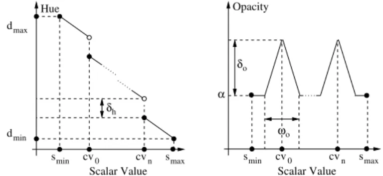
Fig. 6.Transfer function emphasizing topologically equivalent regions
Given a list of critical isovalues we construct a corresponding transfer function based on the methods described by Fujishiro et al. [7]. The domain of the transfer function corresponds to the range of scalar values [smin, smax] occurring in a data set. Outside this range the transfer function is unde-fined. Given a list of critical isovalues cvi, we either construct a transfer function emphasizing volumes containing topologically equivalent isosurfaces or a transfer function emphasizing structures close to critical values.
Fig. 6 shows the construction of a transfer function that emphasizes on topologically equivalent regions. The color transfer is chosen such that hue uniformly decreases with the mapped value, except for a constant drop ofδh at each critical value cvi. The opacity is constant for all values except for hat-like elevations around each critical valuecvi having a width ofωo and a heightδo.
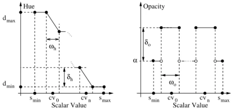
Fig. 7 shows the construction of a transfer function emphasizing details close to critical isovalues. The hue transfer function is constant except for linear descents of a fixed amount δh within an interval with a width ωh centered around each critical isovalue cvi. The opacity is constant for all values except in intervals with a widthωocentered around critical isovalues cvi where the opacity is elevated byδo.
When several isovalues are so close together that intervals with a width ωh orωo would overlap, all isovalues except the first are discarded to avoid
dmax dmin smin cv0 cvn smax δh h ω Scalar Value Hue smin cv0 cvn smax δo ωo α Opacity Scalar Value
Fig. 7. Transfer function emphasizing details close to critical isovalues
high frequencies in the transfer function that could cause aliasing artifacts in the rendered image.
5 Results
Fig. 8 shows the results of rendering a data set resulting from a simulation of fuel injection into a combustion chamber. (Data set courtesy of SFB 382 of the German Research Council (DFG), see http://www.volvis.org for details.) Fig. 8(a) emphasizes on volumes containing topologically equivalent isosurfaces. Details close to these critical isovalues are more visible in Fig. 8(b).
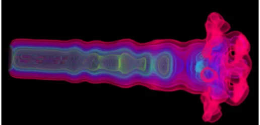
Fig. 9 shows the results of rendering a data set resulting from simulating the spatial probability distribution of the electrons in a high potential protein molecule. Fig. 9(a) emphasizes on volumes containing topologically equivalent isosurfaces. Details close to these critical isovalues are better visible in Fig. 9(b).
6 Conclusions and Future Work
We have presented a method for the detection and utilization of critical isoval-ues for the exploration of trivariate scalar fields defined by piecewise trilinear functions. Improvements to our method are possible. For example, it would be helpful to eliminate the requirement that values at edge-connected vertices of a rectilinear grid must differ. While our approach can be used on data sets that violate this requirement, it fails to detect all critical isovalues for such data. It is necessary to extend our mathematical framework and add the con-cept of “critical regions” and “polylines.” Considering the case of a properly sampled implicitly defined torus, its minimum consists of a closed polyline around which the torus appears. Similar regions of a constant value can exist
that are extrema. These extensions will require us to consider values in a larger region; and they cannot be implemented in a purely local approach. Some data sets contain a large number of critical points. Some of these crit-ical points correspond to locations/regions of actual interest, but some are the result of noise or improper sampling. We need to develop methods to eliminate such “false” critical points.
On the other hand it could be useful to consider more noisy data sets and generate a histogram with the number of topology changes for a lot of small isovalues ranges. It should be possible to automatically detect interesting isovalues by looking for values where there are many topological changes. This could be used to detect turbulence in data sets resulting from unsteady flow simulations in which turbulence is usually associated to “topological noise.” Histograms could also be used to generate meaningful transfer functions for data sets with a large number of closely spaced critical isovalues.
7 Acknowledgments
We thank the members of the AG Graphische Datenverarbeitung und Com-putergeometrie at the Department of Computer Science at the University of Kaiserslautern and the Visualization Group at the Center for Image Pro-cessing and Integrated Computing (CIPIC) at the University of California, Davis.
References
1. Chandrajit L. Bajaj, Valerio Pascucci, and Daniel R. Schikore. The contour spectrum. In: Roni Yagel and Hans Hagen, editors, IEEE Visualization ’97, pages 167–173, IEEE, ACM Press, New York, New York, October 19–24 1997. 2. Chandrajit L. Bajaj, Valerio Pascucci, and Daniel R. Schikore. Visualizing scalar topology for structural enhancement. In: David S. Ebert, Holly Rush-meier, and Hans Hagen, editors, IEEE Visualization ’98, pages 51–58, IEEE, ACM Press, New York, New York, October 18–23 1998.
3. Chandrajit L. Bajaj and Daniel R. Schikore. Topology preserving data simpli-fication with error bounds. Computers & Graphics, 22(1):3–12, 1998.
4. Evgeni V. Chernyaev. Marching cubes 33: Construction of topologically correct isosurfaces. Technical Report CN/95-17, CERN, Geneva, Switzerland, 1995. Available ashttp://wwwinfo.cern.ch/asdoc/psdir/mc.ps.gz.
5. Issei Fujishiro, Taeko Azuma, and Yuriko Takeshima. Automating transfer function design for comprehensible volume rendering based on 3D field topology analysis. In: David S. Ebert, Markus Gross, and Bernd Hamann, editors,IEEE Visualization ’99, pages 467–470, IEEE, IEEE Computer Society Press, Los Alamitos, California, October 25–29, 1999.
6. Issei Fujishiro and Yuriko Takeshima. Solid fitting: Field interval analysis for effective volume exploration. In: Hans Hagen, Gregory M. Nielson, and Frits
Post, editors, Scientific Visualization Dagstuhl ’97, pages 65–78, IEEE, IEEE Computer Society Press, Los Alamitos, California, June 1997.
7. Issei Fujishiro, Yuriko Takeshima, Taeko Azuma, and Shigeo Takahashi. Volume data mining using 3D field topology analysis. IEEE Computer Graphics and Applications, 20(5):46–51, September/October 2000.
8. Thomas Gerstner and Renato Pajarola. Topology preserving and controlled topology simplifying multiresolution isosurface extraction. In: Thomas Ertl, Bernd Hamann, and Amitabh Varshney, editors, IEEE Visualization 2000, pages 259–266, 565, IEEE, IEEE Computer Society Press, Los Alamitos, Cali-fornia, 2000.
9. Gregory M. Nielson. On marching cubes. To appear in IEEE Transactions on Visualization and Computer Graphics, 2003.
10. Gregory M. Nielson and Bernd Hamann. The asymptotic decider: Removing the ambiguity in marching cubes. In: Gregory M. Nielson and Larry J. Rosenblum, editors,IEEE Visualization ’91, pages 83–91, IEEE, IEEE Computer Society Press, Los Alamitos, California, 1991.
11. Hanspeter Pfister, Bill Lorensen, Chandrajit Bajaj, Gordon Kindlmann, Will Schroeder, Lisa Sobierajski Avila, Ken Martin, Raghu Machiraju, and Jinho Lee. The transfer-function bake-off. IEEE Computer Graphics and Applica-tions, 21(3):16–22, May/June 2001.
12. Gunther H. Weber, Gerik Scheuermann, Hans Hagen, and Bernd Hamann. Exploring scalar fields using critical isovalues. In: Robert J. Moorhead, Markus Gross, and Kenneth I. Joy, editors,IEEE Visualization 2002, pages 171–178, IEEE, IEEE Computer Society Press, Los Alamitos, California, 2002.
(a) Transfer function emphasizing topolog-ically equivalent regions.
(b) Transfer function emphasizing struc-tures close to critical isovalues.
Fig. 8.“Nucleon” data set. Data set courtesy of SFB 382 of the German Research Council (DFG), seehttp://www.volvis.org
(a) Transfer function emphasizing topologically equivalent regions.
(b) Transfer function emphasizing structures close to critical isovalues.
Fig. 9.“Neghip” data set. Data set courtesy of VolVis Distribution of SUNY Stony Brook, NY, USA, seehttp://www.volvis.org