Damping of the Second Mode Instability on a Cone in Hypersonic Flow

DAMPING OF THE SECOND MODE INSTABILITY ON A CONE IN HYPERSONIC

FLOW

Sebastian Willems and Ali G ¨ulhan

German Aerospace Center (DLR), Institute of Aerodynamics and Flow Technology, Supersonic and Hypersonic Technology Department, Linder H¨ohe, 51147 K¨oln, Germany, sebastian.willems@dlr.de

ABSTRACT

This paper presents the results of transition experiments

with a3◦half angle cone at Mach6. The transition

po-sition was measured with an infrared camera and simul-taneously the pressure fluctuations in the boundary layer with high speed pressure sensors. A segment with regular micro pores causes a measurable damping of the pressure fluctuations in the boundary layer (Mack modes) but no transition delay. In addition the influence of the nose ra-dius, of the unit Reynolds number and of the free stream temperature on the transition as well as the pressure fluc-tuations is investigated.

Key words: transition; Mack mode; damping; slender cone.

1. INTRODUCTION

The transition from a laminar to a turbulent boundary layer is attended by an increase of the heat flux and drag. An aim of the design of hypersonic vehicles is therefore to delay the transition as long as possible. In hypersonic flows over smooth surfaces the transition is most likely provoked by first and second mode instabilities. As the first modes (Tollmien-Schlichting waves) can be damped by cooled structures, the second modes (Mack modes) become dominant and their damping is the topic of sev-eral research projects. Rasheed et al. [5] could demon-strate a damping of these trapped acoustic waves and a

delay of the transition on a 5◦ half cone with a regular

porous surface at Mach5. Fedorov et al. [2] verified the

damping of the Mack mode with a7◦ half cone and a

porous coating of random micro structures at Mach6.

New transition experiments with a 3◦ half angle cone

at Mach6 were performed in the hypersonic wind

tun-nel (H2K) of the German Aerospace Center (DLR) in

Cologne. The used model is equipped with PCB high

speed pressure sensors and the main parts are made of

polyether ether ketone (PEEK). Therefore simultaneous

measurements of the transition position with an infrared camera and the pressure fluctuations in the boundary

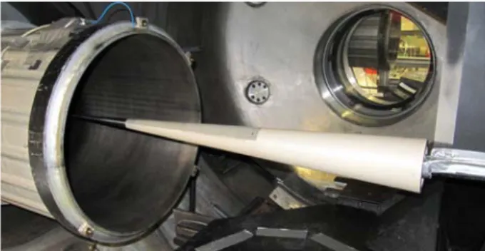
Figure 1. Test section of theH2Kwith the cone model

layer are possible. The dimensions of the micro pores drilled in the surface of one module base on the calcu-lations of Wartemann et al. [9]. They cause a measur-able damping of the pressure fluctuations in the bound-ary layer. The influence of the nose radius is investigated with the help of exchangeable metal apexes. In addition

the operating map of theH2Kallows an examination of

the effect of the unit Reynolds number and of the free stream temperature.

The objective of this paper is a more detailed investiga-tion of the dependencies of the Mack mode including the damping with a regular porous surface.

2. EXPERIMENTAL APPARATUS

2.1. Wind tunnel

The experiments were performed in the Hypersonic wind

tunnel Cologne (H2K) [4]. It is a blowdown wind tunnel

with a free jet test section and a test time of30 s. Figure 1 shows the test section with the model. For the

experi-ments aMach 6contour nozzle with an exit diameter of

600 mmwas used. The inflowing air is heated with resis-tance heaters.

_________________________________________________

Proc. of ‘7th European Symposium on Aerothermodynamics’, Brugge, Belgium 9–12 May 2011 (ESA SP-692, August 2011)

apex middle segment porous surface rear segment Ø 119 mm Ø 99 mm Ø 80 mm Ø 57 mm Ø 36 mm 5c _4c 3c _2c 1c 3a 2a 1a

Figure 2. Sketch of the model parts

2.2. Model

The basic model shape is a 3◦ half angle cone with a

base radius of 60.1 mm. The model consists of three

exchangeable segments - the apex, the middle segment and the rear segment, see also figure 2. The steel apexes

have nose radii of <0.15 mm, 1 mm, 5 mm, 10 mm

and15 mm. Therefore the model length varies between

1146 mmand877 mm. Two middle segments made of

PEEKare in use – one with a plain surface and one with

a generic porous surface formed by regular uniform blind

holes. The holes are80µmin diameter, at least1000µm

in depth and placed every 200µm, thus the porosity is

12.6 %. A close-up is shown in figure 3. The choice of the hole dimensions base on simulations from

Warte-mann with NOLOT [9] [8] and the technical feasibility.

The Fraunhofer Institute for Laser Technology (ILT) in

Aachen performed the manufacturing of these holes with

the help of laser drilling [7] using a pulsed INNOSLAB

laser. In circumferential direction on third (120◦) of the surface is perforated. The perforated area starts at a ra-dius of15.5 mmand ends at a radius of39.5 mm, thus the

porous area has a length of456 mmand contains about

660 000holes. The rear segment of the cone is also made ofPEEK. The model is supported by a central steel shaft.

Figure 3. Close-up of the porous surface

2.3. Instrumentation

The surface temperature on the PEEK segments is

cap-tured via aFLIR SC3000infrared camera [3]. The model is

equipped with four kuliteXCQ-080sensors with a35 kPa

range and a natural frequency of150 kHzfor static and

low speed surface pressure measurements. They are

con-nected to aNI PXIe-4331 bridge module. For high speed

Figure 4. Surface temperature increase @ M a= 6.0,

rN = 0.15,Re= 4·106 1_m,T0= 500 K, plain

pressure measurements the model is equipped with eight

PCB 132A31 sensors (their positions are marked in

fig-ure 2) with a350 kPa range and a resonant frequency

above1 MHz. They are connected to charge amplifiers

PCB 482C05 and their output signals are measured with AdlinkPXI-9816D/512digitizers.

2.4. Data preparation

The raw data of the infrared camera are trans-ferred into surface temperatures using ThermaCAM Re-searcher 2001. Then the temperature values along the symmetry line of the model are extracted. Afterwards the values of the last picture before the wind tunnel start is

subtracted from the values12 slater. The X-coordinates

are transformed into the path length from the apex which splits into the arc length and the generatrix. With equa-tion (1) the path lengthlon a cone with the half angleα

(hereα= ₆₀π) and the nose radiusrN can be calculated

based on the cone radiusrBat this position.

l= rB sin (α)− rN tan (α)+rN· π 2 −α (1)

The frequency spectra of thePCBsensors, shown in this

paper, base on measurements with a sampling rate of

4 MHzand a measurement period at stable flow

condi-tions of 15 s. The gained data are divided into 5999

blocks with 20 000samples each. The blocks overlap

each other by50 %. Each block is multiplied with the

Hann function and afterwards Fourier transformed. The arithmetic mean of all block results is then scaled with the static pressure of the inflow. The frequency spectra show root mean square values.

3. RESULTS

3.1. Reynolds number

Figure 5 shows the temperature increase on the plain

PEEKsegments of the cone with a nose radius of0.15 mm

for three different Reynolds numbers. The transition re-gion can be located with the help of the typical increase

Re = 4·10 1/m6 Re = 6·10 1/m6 Re = 12·10 1/m6 PCB 5a PCB 3a PCB 4a PCB 1a sensor positions: PCB 2a X [mm] ∆ T @ 1 2 s [K ] 0 200 400 600 800 1000 1200 0 10 20 30 40 50 PCB 1a PCB 2a PCB 3a PCB 4a PCB 5a dT [K]: V239: Ma = 6.0 r = 0.1 mm Re = 4e6 T = 500 K plain dT [K]: V238: Ma = 6.0 r = 0.1 mm Re = 6e6 T = 500 K plain dT [K]: V212: Ma = 6.0 r = 0.1 mm Re = 12e6 T = 500 K plain

Figure 5. Surface temperature increase dependent on Reynolds number @ M a= 6.0, rN = 0.15 mm,

T0= 500 K, plain

of the surface temperature. For a Reynolds number of

4·106 1

m the transition takes place at a path length of

620to1020 mm, for6·106 1

m at500to750 mmand for

12·106 1

m at340 to440 mm. Thus with an increasing Reynolds number the length of the transition region de-creases and moves upstream.

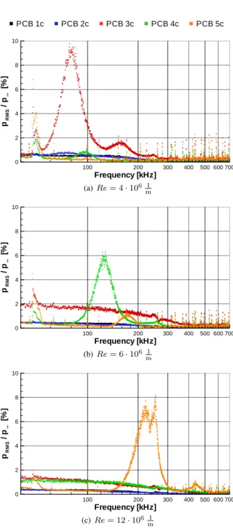
The pressure frequency spectra are shown in the figures 6(a)-(c). Their positions are also marked in figure 5. The

significant peak at50 kHzis no flow phenomenon as it

appears also at reference measurements in vacuum. Nev-ertheless, the peaks of the Mack mode are quite obvious and its increase and destruction can be observed.

For the case with a Reynolds number of 4 · 106 1_m

(fig. 6(a)) there is nothing interesting in the spectrum of the first sensor (PCB5c) at a path length of339 mm. At a path length of545 mm, this is still before the transi-tion, the sensor 4c registers a small peak at100 kHz. At

a path length of 762 mm(PCB3c), this is at the

begning of the transition, supposable the same peak has

in-creased to10%of the static pressure and moved to a

fre-quency of80 kHz. In addition a second smaller peak has

formed at a frequency of 160 kHz. At a path length of

947 mm(PCB2c), this is towards the end of the transi-tion, the peak disappeared almost completely. There is

just a small bump at75 kHz. The frequency spectrum of

the last sensor (PCB5c) at a path length of1133 mmis

again completely even.

The situation for the two other Reynolds numbers is sim-ilar, but some differences are noticeable. As indicated by the temperature profiles, all effects move upstream. With a Reynolds number of6·106 1

m(fig. 6(b)) the first peak of

the Mack modes is registered byPCB5c and the biggest

peak byPCB4c. PCB3c which is at the end of the

tran-sition region measures a broad increase of the pressure

amplitudes for frequencies below300 kHz. In

compari-son to the6·106 1

mcase the frequency of the Mack mode

at the same path lengths increases (175 kHz at PCB5c

and125 kHzatPCB4c). The reduced maximum ampli-tude and the hardly detectable second peak are not sig-nificant, as they highly depend on the sensor position in

PCB 1c PCB 2c PCB 3c PCB 4c PCB 5c Frequency [kHz] pR M S / p∞ [% ] 100 200 300 400 500 600 700 0 2 4 6 8 10 (a)Re= 4·106 1 m Frequency [kHz] pR M S / p∞ [% ] 100 200 300 400 500 600 700 0 2 4 6 8 10 (b)Re= 6·106 1 m Frequency [kHz] pR M S / p∞ [% ] 100 200 300 400 500 600 700 0 2 4 6 8 10 (c) Re= 12·106 1 m

Figure 6. Pressure frequency spectra dependent on sen-sor position @M a= 6.0,rN = 0.15 mm,T0= 500 K,

relation to the transition position. At a Reynolds num-ber of12·106 1

m the maximum amplitude of the second

Mack mode is registered fromPCB5c at a still higher

fre-quency around240 kHz. In addition there is again a

dis-tinctive second peak at440 kHz. This timePCB4c and 3c

measure a broad increase of the pressure amplitudes for

frequencies below300 kHz. The reduced noise level at

higher Reynolds number is caused by the higher pressure level.

3.2. Nose radius

Figure 7 shows the temperature increase on the plain cone

for several nose radii. The observed region of thePEEK

segments shifts regarding the path length, because of the different length of the nose segments. It is obvious that the smaller the nose radius the earlier and the shorter is the transition region.

r = 0.15 mmN r = 1.0 mmN r = 5.0 mmN r = 10.0 mmN sensor positions: r = 0.15 mmN r = 1.0 mmN r = 5.0 mmN r = 10.0 mmN X [mm] ∆ T @ 1 2 s [K ] 0 200 400 600 800 1000 1200 0 10 20 30 40 50

Figure 7. Temperature increase dependent on nose radius @M a= 6.0,Re= 12·106 1 m,T0= 500 K, plain PCB 5c r = 0.15 mmN PCB 4c r = 1.0 mmN PCB 3c r = 5.0 mmN PCB 2c r = 5.0 mmN PCB 2c r = 10.0 mmN PCB 1c r = 10.0 mmN Frequency [kHz] pR M S / p∞ [% ] 100 200 300 400 500 600 700 0 2 4 6 8 10

Figure 8. Pressure frequency spectra dependent on nose radius @M a = 6.0,Re = 12·106 1

m,T0 = 500 K,

plain

Due to the different nose lengths and the different

tran-sition potran-sitions a comparison of the pressure frequency spectra is difficult. The pressure frequency spectra of the positions marked in figure 7 are shown in figure 8. With

a nose radius of0.15 mmPCB5c at the beginning of the

transition region registers the already described

conspic-uous peak. With a nose radius of 1 mm PCB4c in the

middle of the transition region registers a smaller, less

sharp peak at a lower frequency of150 kHzbut with a

distinctive second peak at260 kHz. For a nose radius of

5 mmas well as for10 mmneither at the beginning of the

transition region (PCB3c respectivelyPCB2c) nor at the end of the transition region (PCB2c respectivelyPCB1c) there are any noticeable peaks.

3.3. Temperature

Figure 9 shows, that a change of the temperature level with the same Reynolds number has no effect on the tran-sition potran-sition. But figure 12 shows, that with the increas-ing temperature the frequency and the amplitude of the measured Mack mode increase.

T = 500 K0 T = 600 K0 T = 770 K0 sensor position: PCB 3c X [mm] ∆ T @ 1 2 s [K ] 0 200 400 600 800 1000 1200 0 10 20 30 40 50 60 70 PCB 3c dT [K]: V209: Ma = 6.0 r = 1.0 mm Re = 4e6 T = 500 K plain dT [K]: V218: Ma = 6.0 r = 1.0 mm Re = 4e6 T = 600 K plain dT [K]: V216: Ma = 6.0 r = 1.0 mm Re = 4e6 T = 770 K plain

Figure 9. Temperature increase dependent on tempera-ture @M a= 6.0,rN = 1.0 mm,Re= 4·106 1_m, plain T = 500 K0 T = 600 K0 T = 770 K0 Frequency [kHz] pR M S / p∞ [% ] 100 200 300 400 500 600 700 0 2 4 6 8 10

PCB 3c / Pstat [%]: V221: Ma = 6.0 r = 1.0 mm Re = 4e6 T = 500 K porous PCB 3c / Pstat [%]: V229: Ma = 6.0 r = 1.0 mm Re = 4e6 T = 600 K porous PCB 3c / Pstat [%]: V231: Ma = 6.0 r = 1.0 mm Re = 4e6 T = 770 K porous

Figure 10. Pressure frequency spectra dependent on tem-perature @M a= 6.0, rN = 1.0 mm, Re= 4·106 1_m,

3.4. Perforation

The effect of the porous surface was measured by replac-ing the middle section as a rotation of the whole model comes along with the need of an angle of attack adjust-ment. The experience of adjusting the yaw angle via the infrared images shows the high sensitivity of the transi-tion positransi-tion to the angle of attack. Another advantage is that the samePCBsensors are in use. But the result is that the porous surface has nearly no effect on the transition position. Figure 11 shows that it even tends to an earlier transition. Nevertheless figure 12 shows a significantly reduced amplitude of the Mack mode in the middle of the transition region. The amount of the damping is about

36%.

plain porous sensor position: PCB 3a

X [mm] ∆ T @ 1 2 s [K ] 0 200 400 600 800 1000 1200 0 10 20 30 40 50 PCB 3a dT [K]: V242: Ma = 6.0 r = 0.1 mm Re = 4e6 T = 500 K plain dT [K]: V243: Ma = 6.0 r = 0.1 mm Re = 4e6 T = 500 K porous

Figure 11. Temperature increase dependent on sur-face @ M a= 6.0, rN = 0.15 mm, Re= 4·106 1_m, T0= 500 K plain porous Frequency [kHz] pR M S / p∞ [% ] 100 200 300 400 500 600 700 0 2 4 6 8 10

PCB 3a / Pstat [%]: V242: Ma = 6.0 r = 0.1 mm Re = 4e6 T = 500 K plain PCB 3a / Pstat [%]: V243: Ma = 6.0 r = 0.1 mm Re = 4e6 T = 500 K plain

Figure 12. Pressure frequency spectra dependent on surface @M a= 6.0, rN = 0.15 mm,Re= 4·106 1_m,

T0= 500 K

4. CONCLUSION

The results of the Reynolds number, nose radius and temperature variations concerning the transition position met the expectations and agree with former investigations as from M¨uller and Henckels [3]. An increase of the Reynolds number or a decrease of the nose radius short-ens the transition region and moves it upstream. A change

of the temperature level in the examined range has no ef-fect on the transition. A delay of the transition due to the porous surface as observed by Rasheed et al. [5] could not be measured.

More interesting are the measured pressure frequency spectra. The Mack mode is detectable before the tran-sition process starts and its amplitude increases to maxi-mum within the transition region. It becomes completely destructed with the completion of the transition process. With increasing path length the frequency of the Mack mode decreases. When the Mack mode is strongly am-plified a second peak forms at about twice the frequency of the main peak, and thus can be identified as its1st

har-monic. These effects are also visible in the measurements of Roediger et al. [6] and Berridge et al. [1]. The in-crease of the Mack mode’s frequency with the Reynolds number also agrees to the results of Berridge. The in-fluence of the nose radius on the Mack mode has to be interpreted carefully. The results indicate that the Mack mode develops just with small nose radii and an increase of the nose radius reduces its frequency. The increase of the frequency with the temperature is self-evident and quantitative matches the increase of the speed of sound with the root of the temperature. Although the amplitude increase is small it has been confirmed with other

experi-ments using a nose radius of0.15 mm.

Although the transition delay could not be measured, the damping of the Mack mode with the help of a regular porous surface could be verified. The amount of damp-ing is in good agreement with the calculations done by Wartemann et al. [10].

For a more detailed investigation of the amplification and destruction of the Mack mode it would be interesting to increase the number ofPCBsensors in a row. To verify the experience of Rasheed et al. [5], which show that a tran-sition delay requires lower Reynolds numbers, a porous rear segment is needed as the transition region moves downstream. Experiments at other Mach numbers could generalize the results.

ACKNOWLEDGMENTS

These experiments are part of theDLR research project

IMENS-3C. Special thanks go to Mr. Brajdic from the

ILTin Aachen for his great personal commitment for the

realization of the porous surface. Thanks also toPJKin

Sankt Augustin for accepting the challenge of turning a

sharp3◦nose. Last but not least the commitment of the

technical staff of theH2Kis gratefully acknowledged.

REFERENCES

[1] Berridge, D. C., Casper, K. M., Rufer, S. J., Alba, C. R., Lewis, D. R., Beresh, S. J., and Schneider, S. P. (2010). Measurements and Computations of Second-Mode Instability Waves in Three Hypersonic Wind

Tunnels. In40th Fluid Dynamics Conference and Ex-hibit, AIAA, Chicago. American Institute of Aeronau-tics and AstronauAeronau-tics.

[2] Fedorov, A. V., Shiplyuk, A. N., Maslov, A. A., Burov, E. V., and Malmuth, N. D. (2003). Stabiliza-tion of a hypersonic boundary layer using an ultrason-ically absorptive coating. Journal of Fluid Mechanics, 479:99–124.

[3] M¨uller, L. and Henckels, A. (1997). Visualization of High Speed Boundary Layer Transition with FPA

Infrared Technique. InNotes on Numerical Fluid

Me-chanics, volume 60, pages 245–252.

[4] Niezgodka, F.-J. (2001). Der Hyperschallwindkanal

H2K des DLR in K¨oln-Porz (Stand 2000). DLR-Mitteilungen. Deutsches Zentrum f¨ur Luft- und Raum-fahrt e. V., K¨oln.

[5] Rasheed, A., Hornung, H. G., Fedorov, A. V.,

and Malmuth, N. D. (2002). Experiments on

Pas-sive Hypervelocity Boundary-Layer Control Using an

Ultrasonically Absorptive Surface. AIAA Journal,

40(3):481–489.

[6] Roediger, T., Knauss, H., Estorf, M., Schneider, S. P., and Smorodsky, B. V. (2009). Hypersonic In-stability Waves Measured Using Fast-Response

Heat-Flux Gauges. Journal of Spacecraft and Rockets,

46(2):266–273.

[7] Walther, K., Brajdic, M., Kelbassa, I., and Poprawe,

R. (2008). Bohren mit gepulster Laserstrahlung. wt

Werkstattstechnik online, 98(6):520–523.

[8] Wartemann, V. and L¨udeke, H. (2010). Investiga-tion of Slip Boundary CondiInvestiga-tions of Hypersonic Flow over Microporous Surfaces. In Pereira, J. C. F. and

Se-queira, A., editors, V European Conference on

Com-putational Fluid Dynamics, number June, Lisbon. [9] Wartemann, V., L¨udeke, H., and Sandham, N. D.

(2009). Stability analysis of hypersonic

bound-ary layer flow over microporous surfaces. In 16th

AIAA/DLR/DGLR International Space Planes and Hy-personic Systems and Technologies Conference, pages 1–10.

[10] Wartemann, V., L¨udeke, H., Willems, S., and

G¨ulhan, A. (2011). Stability Analyses and

Valida-tionof a Porous Surface Boundary Condition by

Hy-personic Experiments on a Cone Model. In7th

Euro-pean Aerothermodynamics Symposium, Brugge. ESA Publications Division.