Ritos, Konstantinos and Kokkinakis, Ioannis W. and Drikakis, Dimitris
(2018) Performance of high-order implicit large eddy simulations.
Computers and Fluids, 173. pp. 307-312. ISSN 0045-7930 ,
http://dx.doi.org/10.1016/j.compfluid.2018.01.030
This version is available at https://strathprints.strath.ac.uk/63146/
Strathprints
is designed to allow users to access the research output of the University of
Strathclyde. Unless otherwise explicitly stated on the manuscript, Copyright © and Moral Rights
for the papers on this site are retained by the individual authors and/or other copyright owners.
Please check the manuscript for details of any other licences that may have been applied. You
may not engage in further distribution of the material for any profitmaking activities or any
commercial gain. You may freely distribute both the url (
https://strathprints.strath.ac.uk/
) and the
content of this paper for research or private study, educational, or not-for-profit purposes without
prior permission or charge.
Any correspondence concerning this service should be sent to the Strathprints administrator:
[email protected]
The Strathprints institutional repository (https://strathprints.strath.ac.uk) is a digital archive of University of Strathclyde research outputs. It has been developed to disseminate open access research outputs, expose data about those outputs, and enable the
Contents lists available at ScienceDirect
Computers
and
Fluids
journal homepage: www.elsevier.com/locate/compluid
Performance
of
high-order
implicit
large
eddy
simulations
Konstantinos Ritos
∗, Ioannis W. Kokkinakis
, Dimitris Drikakis
∗ UniversityofStrathclyde,Glasgow,G11XJ,UKa
r
t
i
c
l
e
i
n
f
o
Articlehistory:
Received24January2017 Revised30October2017 Accepted23January2018 Availableonline31January2018
Keywords: iLES High-Ordermethods Turbulentflows Parallelcomputing
a
b
s
t
r
a
c
t
Theperformance ofparallelimplicit LargeEddySimulations(iLES) isinvestigated inconjunctionwith high-orderweightedessentiallynon-oscillatoryschemesupto11th-orderofaccuracy.Simulationswere performedfortheTaylorGreenVortexand supersonicturbulentboundarylayerflows onHigh Perfor-manceComputing(HPC)facilities.ThepresentiLESarehighlyscalableachievingperformanceof approx-imately93%and68%on1536and6144cores,respectively,forsimulationsonameshofapproximately 1.07billioncells.Thestudyalsoshowsthathigh-orderiLES attainaccuracysimilar tostrictDirect Nu-mericalSimulation(DNS)butatareducedcomputationalcost.
© 2018TheAuthors.PublishedbyElsevierLtd. ThisisanopenaccessarticleundertheCCBYlicense.(http://creativecommons.org/licenses/by/4.0/)
1. Introduction
Implicit Large Eddy Simulations (iLES) originated from the ob- servations made in [1] that the embedded dissipation of a certain class of numerical methods can be used in lieu of the explicit Sub- Grid Scale (SGS) models. Modified Equation Analysis (MEA) was developed [2] aiming at determining the stability of a difference equation by examining the truncation errors. Such an analysis was performed for the truncation error of certain schemes, e.g., [3–9] ) leading to a better understanding of the implicit sub-grid dissi- pation. In iLES, the Navier–Stokes Equations (NSE) are discretised using high-resolution methods without involving a low-pass filter- ing operation, which leads to SGS terms that require additional modelling. Instead, only the (implicit) de facto filtering introduced through the finite volume integration of the NSE over the mesh cells is utilised in conjunction with non-linear numerical schemes that adhere to a number of principles; see [10,11] , and reviews
[9,12,13] . It has been shown [7] that iLES methods need to be care- fully designed, optimised, and validated for the particular differen- tial equation to be solved. Direct MEA of high-resolution schemes for NSE is difficult to be performed, thus understanding of the nu- merical properties of these methods to date still relies on perform- ing computational experiments.
The use of iLES in free and wall-bounded flows has been justi- fied by several authors [14,15] , while a validation of the approach through theoretical analysis has been presented by Margolin et al.
[8] . In incompressible flows, it is possible to develop an optimised
∗ Correspondingauthors.
E-mail addresses: [email protected] (K. Ritos),
[email protected](D. Drikakis).
stencil with regards to numerical dissipation [16] , however, in the case of compressible flows the numerical method should be mono- tonic with respect to the thermodynamic quantities. Poggie et al.
[17] and Ritos et al. [18] applied compressible iLES to study Turbu- lent Boundary Layer (TBL) flows and showed that iLES can achieve close to strict DNS (see page 4 for definition of strict DNS) accuracy on significantly coarser meshes. Despite iLES (and similarly classi- cal LES) being computationally less demanding than DNS, it still re- quires significant computational resources for simulating near-wall turbulence at high Reynolds numbers.
To date, there has been no systematic attempt to investigate the parallel scalability of different high-order compressible iLES meth- ods in free and wall-bounded flows. The aim of this study is to present results regarding the accuracy, efficiency and parallel scal- ability of high-order iLES with reference to the Taylor Green Vortex (TGV) and supersonic TBL flows.
2. Numericalmethodsandflowcases
We have employed iLES in the framework of the CFD code CNS3D [12,15] . The Navier–Stokes equations are solved by using a finite volume Godunov-type method for the convective terms, which comprises the HLLC approximate Riemann solver [13,19] and two high-resolution schemes. The Monotone Upstream-centered Scheme for Conservation Laws (MUSCL) with second-order piece- wise linear monotonised central limiter [20] (labelled as M2), and the Weighted-Essentially Non-Oscillatory (WENO) ninth-order scheme [21] (labelled as W9). Furthermore, in order to exam- ine the parallel scalability of high-order iLES, simulations were also performed using an eleventh-order WENO scheme (labelled as W11).
https://doi.org/10.1016/j.compfluid.2018.01.030
308 K.Ritosetal./ComputersandFluids173(2018)307–312
Table1
Simulationparameters:u∞,T∞,M,P∞,ρ∞,andμ∞arethefreestream
velocity,temperature,Machnumber,pressure,densityandviscosity, respectively.Tw isthewalltemperature,Iistheturbulenceintensity
attheinletandReListheReynoldsnumberbasedonthefreestream
propertiesofairandtheplatelength,L.
L u∞ T∞ M P∞
0.061m 588m/s 170K 2.25 23.8kPa
ρ∞ Tw/T∞ μ∞ I ReL
0.488kg/m3 1.9 1.167×10⁻⁵Pas 3% 1.5×10⁶
The viscous terms are discretised using a second-order cen- tral scheme. The solution is advanced in time using a five-stage (fourth-order accurate) optimal strong-stability-preserving Runge– Kutta method [22] . Further numerical details are provided in
[15] and references therein.
The first flow case considered here is the TGV in a triple- periodic cubic domain of length 2
π
(m). A series of meshes was used: 32 3, 64 3, 128 3, 256 3 and 512 3 evenly-spaced computationalcells. The flow is initialised by solenoidal velocity profile,
u0=U0sin
(
kx)
cos(
ky)
cos(
kz)
,v
0=−U0cos(
kx)
sin(
ky)
cos(
kz)
,w0=0,
(1)
and the pressure is obtained by solving the Poisson equation:
P0=P∞+
1 16
ρ
0U2
0[2+cos
(
2kz)
]·[cos(
2kx)
+cos(
2ky)
], (2)where the wavenumber k=1 . An ideal gas equation of state is used and the Mach number, U0/
γ
P0/ρ
0, is 0.08. The results arepresented in terms of non-dimensional units; distance x∗=kx and time t∗=kU0t.
The second flow case considered here is a supersonic turbu- lent flow over a flat plate at Mach number M=2 .25 and Reynolds number of 1.5 ×10 6based on the freestream properties for air and
the length of the plate, L; see also Table 1 .
Periodic boundary conditions are used in the spanwise direction (z). In the wall-normal direction (y) a no-slip isothermal wall at temperature Tw=323 K is imposed. Supersonic outflow conditions are applied at the outlet, while far-field conditions are applied on the upper boundary opposite to the wall.
A synthetic turbulent inflow boundary condition is used to pro- duce a freestream flow with a superimposed random turbulence. The synthetic turbulent inflow boundary condition is based on the digital filter (DF) method [18,23–25] . According to DF, instead of using a white-noise random perturbation at the inlet, energy modes within the Kolmogorov inertial range scaling with k−5/3
, where k is the wavenumber, are introduced into the turbulent boundary layer. A cutoff at the maximum frequency of 50 MHz is applied since the finest mesh would under-resolve higher fre- quency values. The turbulence intensity at the inlet ( I) is set as
±3% of the intensity of the freestream velocity. This perturbation has been found to be sufficient to trigger bypass transition and tur- bulence downstream (see Fig. 1 ).
iLES have been performed on fine meshes but still coarser than DNS [17,26] . We employed four meshes with the coarsest and finest meshes containing ∼4.5 million and ∼100 million cells, re- spectively. For the calculation of the mesh spacing
y
the con- ventional inner variable scaling methody
+=uτy
/ν
w is used,where uτ=√
τ
w/ρ
w is the friction velocity;ν
w,τ
w andρ
w are the wall viscosity, shear stress and density, respectively. Typical mesh resolution recommendations for LES lie in the range of 50 <x
+<150 and 15 <z
+< 40 , and for DNS in the range of 10 <x
+<20 and 5 <z
+<10 [17,27,28] . For wall-resolved LES andDNS the near-wall spacing should be
y
+< 1 . A strict definitionTable2
Boundarylayerproperties,includingpreviousDNSand experimen-talstudies.Thecompressibleformofthemomentumthickness(θ) hasbeenusedinthedefinitionofReθandReδ2.Reτ istheReynolds
numberbasedonthefrictionvelocityuτ andtheboundarylayer
thicknessδ.Reδ2 isbasedonθ and thenear-wallviscosity μw. H= δ∗/θ istheshapefactor,whereδ∗isthedisplacement
thick-nessofcompressibleflow.
Reθ Reτ Reδ2 H M W9 2170.0 414.0 1280.6 3.56 2.25 M2 1593.8 344.6 940.5 3.72 2.25 DNS[26] 2377.0 497.0 1516.0 2.98 2.0 strictDNS[17] - - 2000.0 - 2.25 Exp[29] 5100.0 1080.0 3100.0 2.00 2.28
for DNS mesh spacing requires
x
+≤1 andy
+≤1 . The mesh spacing used in this study is in the range of 9 .06 <x
+< 27 .14 ,0 .497 <
y
+<1 .22 and 8 .53 <z
+< 24 .95 , where the smallestvalues correspond to the finest mesh. Based on the above analy- sis, the present iLES on the finest mesh can be considered as an under-resolved DNS.
The TBL properties are presented in Table 2 . To enable the com- parison of the present results with other publications, various def- initions of the Reynolds number have been employed based on the momentum thickness, the friction velocity, and the near-wall vis- cosity. The flow statistics are computed by averaging in time over three flow cycles and, spatially, in the spanwise direction. The sta- tistical convergence of the simulations based on the standard error of the mean is less than 2%.
3. Results 3.1. TGV
Instantaneous visualisations of the TGV at t∗=15 ( Fig. 2 ) show
the dominance of disorganised vortices in the decaying worm- vortex flow regime. The results were obtained using the ninth- order WENO scheme on 64 3, 128 3, 256 3 and 512 3 meshes. The
snapshots of the flow are based on the Q-criterion, which defines a vortex as a continuous fluid region with a positive second invariant of the velocity gradient [30] , i.e. Q>0. All renderings are performed at the same level ( Q= 1 ) and are coloured with the velocity mag- nitude.
The results on 256 3 and 512 3meshes are very similar with re-
spect to the turbulent structures resolved. The kinetic energy rate of dissipation,
ε
1, and pressure dilation-based dissipation rate,ε
2,are shown in Fig. 3 . The kinetic energy rate of dissipation is calcu- lated by
ε
1=−dEk/dt, where Ek= 1ρ
0V 1 2ρ
u·udV (3)is the volumetric-averaged kinetic energy. The simulations are nearly grid converged with respect to
ε
1 and agree with otherpublished results [31,32] (not shown here). The pressure dilatation- based dissipation rate is defined by
ε
2=− 1ρ
0V
p
∇
·udV. (4)ε
2measures the effect of compressibility on the dissipation of tur-bulent energy and takes small values for low Mach flows.
A widely used performance metric for assessing parallel com- putations is the speedup:
Sn=
Tre f
Tn
, (5)
where Tn is the execution time on n cores and Trefis the execution time on a reference number of processors, usually equal to a single
(a)
(b)
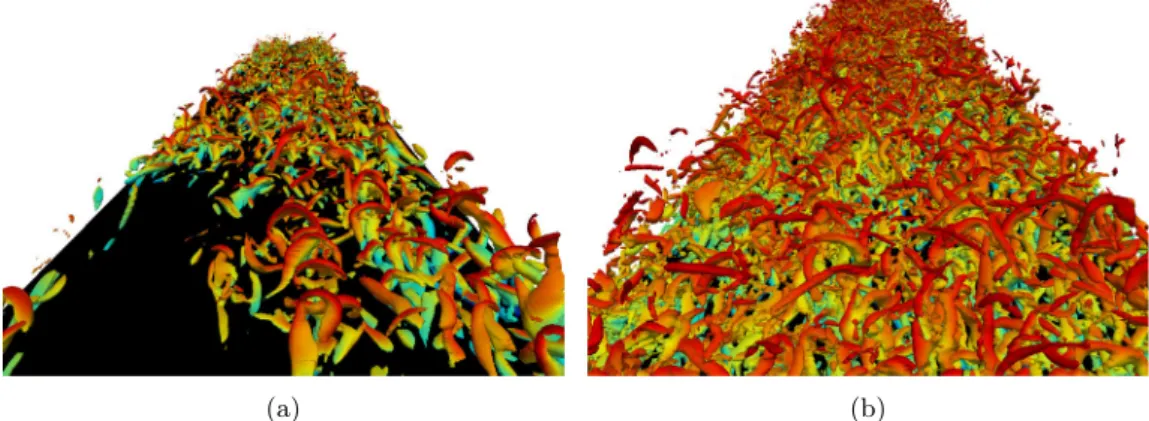
Fig.1. Iso-surfacesofQ-criterion,colouredbyMachnumber,for(a)M2and(b)W9iLESsimulations;thecomputationaldomainhasbeentruncated.(Forinterpretationof thereferencestocolourinthisfigurelegend,thereaderisreferredtothewebversionofthisarticle).
(a) mesh = 64
3(b) mesh = 128
3(c) mesh = 256
3(d) mesh = 512
3Fig.2. Iso-surfacesofQ-criterion(Q = 1)colouredbyvelocitymagnitudeatt∗= 15.The323meshisnotshownasnostructureisvisibleatthislevelofQ.AllshownTGV simulationsarewithW9.(Forinterpretationofthereferencestocolourinthisfigurelegend,thereaderisreferredtothewebversionofthisarticle).
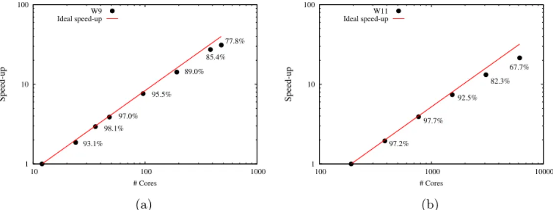
core or to the number of cores in a computational node of the HPC facility used. For the TGV simulations on meshes up to 512 3 cells,
12 cores were used as reference; one HPC node has two Intel Xeon X5650 processors with 6 cores each. The ideal speedup of paral- lel computations would be equal to n/ nref, but this efficiency is not possible due the communication overhead between the computa- tional cores and the idle time of computational nodes associated with load balancing. Fig. 4 a shows the parallel speedup for the TGV case using the ninth-order iLES, achieving 77% speed-up using 480 cores. Furthermore, for scalability purposes the parallel per- formance of the eleventh-order WENO iLES on 6144 cores for the 1024 3 simulation is shown; a Cray HPC facility compromising two
Intel E5-2697v2 processors with 12 cores each was used. The refer- ence execution time was obtained on 192 cores. The parallel per- formance of the 1024 3 simulation is approximately 93% and 68%
on 1536 and 6144 cores, respectively. The parallel performance of the second-order iLES is not shown because it involves less calcu- lations for the same mesh size and as a consequence the scalability will always be worse when comparing to higher order iLES. 3.2.TBL
The second flow case is a supersonic TBL for which DNS re- sults and experimental data at similar Mach numbers are available.
310 K.Ritosetal./ComputersandFluids173(2018)307–312
Fig.3. TGVcase:(a)Kineticenergydissipationrate(ε1)and(b)pressuredilatation-baseddissipationrate(ε2).Theresultsonthe5123meshareincloseagreementwith previouslypublishedresults[31,32](notshownhere).They-axisin(b)isstretchedbyafactorof10comparedto(a).
Fig.4. Parallelscalingof(a)9th-and(b)11th-orderiLESfortheTGVcaseon1283and10243meshes,respectively.
Fig.5. ComparisonofiLESwithDNSandexperimentaldata.(a)vanDriestvelocityprofile(b)normalReynoldsstress.StrictDNSresults[17]areincludedonlyin(b)because forthevelocityprofilestheresultsperfectlyagreewiththeavailableDNSdataofPirozzolietal.[26].“LR” denotesalowerresolutionmeshcontainingapproximately1/3of thesizeofthefinemesh.
Comparisons with DNS and/or experiments are presented for the van Driest velocity profile, uVD, and normal Reynolds stress,
τ
uu ( Fig. 5 ). The van Driest velocity profile is given byuVD= u+ 0
ρ
ρ
w du+, (6)where the superscript ‘ +’ denotes wall scalling, u+=u/uτ. Previ-
ous publications [26,33] have shown that for adiabatic walls a sat- isfactory agreement of the velocity data is expected in near-wall region. Small variations are expected for different Reynolds num- ber and the present iLES are in agreement with the DNS of Piroz- zoli et al. [26] . The ninth-order iLES is also in excellent agreement with the experimental data [29] . The second-order iLES, conducted on the same mesh resolution, shows significant deviation from the
reference DNS and experiments. Performing the ninth-order iLES on 1/3 mesh resolution shows that mesh convergence is achieved, hence the high-order iLES reliably attain high accuracy on a rela- tively coarse mesh.
In respect of
τ
uu, the second-order iLES significantly over- estimate the Reynolds normal stress, especially in the peak region of the buffer zone. The ninth-order iLES show very good agreement with the DNS results up to about y+≈20 , where the Reynoldssimilarity holds [34] . Further away from the wall it is typical to observe a strong dependence on Reynolds number for results pre- sented in inner scaling coordinates. This explains the differences in the results in the logarithmic region due to the differences in the local Reynolds number.
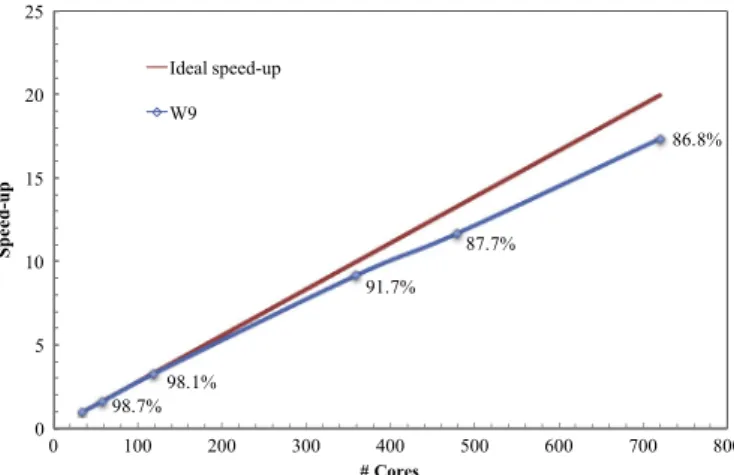
Fig.6. iLESspeed-upforthe9th-orderWENOschemeforthesupersonicTBLcase. Table3
PerformanceofsecondandninthorderiLESvsDNS[17,26]. Method Computationalcost Error1 Error2
StrictDNS ∼25(years) 0.0% 0.0%
DNS 117(days) 0.0% 6.5%
iLESW9 24(days) 1.0% 6.3%
iLESM2 10(days) 8.5% 23.7%
iLESW9-LR 7(days) 3.1% 8.1%
For the TBL case the speedup is calculated with reference to 36 cores (3 computational nodes with two Intel Xeon X5650 proces- sors each node). The 36 cores reference was imposed due to the size of the fine mesh ( ∼100 million cells). The parallel speedup is shown in Fig. 6 . The ninth-order iLES provide a computational ef- ficiency of 86% of the ideal efficiency, utilising 720 computational cores.
Table 3 shows the performance of low and high order iLES with reference to strict DNS [17] . For the DNS performance we have used the results of Pirozzoli et al. [26] , where a mesh ap- proximately 27 times coarser than the strict definition of DNS was utilised. The reported errors are averaged values calculated in the near-wall region, y+≤30 , where “Error1” and “Error2” refer to
relative difference from the reference van Driest velocity profile and normal wall stress, respectively. The computational cost has been calculated based on the assumption that simulations are per- formed on 240 cores. The computational cost for DNS are estima- tions based on the mesh size and number of cores found in the relevant publications. The results show that high-order iLES can at- tain high accuracy at a reduced computational cost, cf. iLES W9-LR with the rest of the results.
4. Conclusions
The accuracy, parallel scalability and efficiency of iLES were ex- amined for different turbulent flow cases. A mesh convergence study was presented for the TGV case achieving nearly mesh inde- pendent results for the two finest meshes. The present high-order iLES exhibit high parallel efficiencies for simulations performed up to 6144 cores on a Cray HPC facility and for meshes containing up to 1.07 billion cells.
The first and second order statistics obtained from high-order iLES of a supersonic TBL flow are in excellent agreement with pre- vious numerical and experimental data. iLES can achieve high ac- curacy in the near-wall region that is directly comparable to the results of strict DNS at a reduced computational cost. A combina- tion of high-order iLES with relatively coarse meshes provides a
more pragmatic approach than using a second order method on a significantly finer mesh.
Acknowledgements
Results were obtained using the EPSRC funded ARCHIE-WeSt High Performance Computer ( www.archie-west.ac.uk ) under EPSRC grant no. EP/K0 0 0586/1 . The authors would also like to thank EP- SRC for providing access to computational resources on the Na- tional HPC facility ARCHER through the UK Applied Aerodynamics Consortium Leadership Project “e529”.
References
[1] BorisJ,GrinsteinFF,OranE,KolbeR.Newinsightsintolargeeddysimulation. FluidDynRes1992;10(4–6):199–228.
[2] HirtC.Heuristicstabilitytheoryforfinite-differenceequations.JComputPhys 1968;2(4):339–55.
[3] MargolinLG,RiderWJ.Arationaleforimplicitturbulencemodelling.IntJ Nu-merMethods2002;39(9):821–41.
[4] Rider WJ, MargolinLG. Fromnumericalanalysis toimplicit subgrid turbu-lencemodeling.In:16thAIAAcomputationalfluiddynamicsconference;2003. p.1–11.
[5] Drikakis D, Rider WJ. High-resolution methods for incompressible and low-speedflows,1.Springer-Verlag;2004.
[6] MargolinLG,RiderWJ.ThedesignandconstructionofimplictLESmodels.Int JNumerMethods2005;47(10–11):1173–9.
[7] DomaradzkiJA,RadhakrishnanS.Effectiveeddyviscositiesinimplicit model-ingofdecayinghighReynoldsnumberturbulencewithandwithoutrotation. FluidDynRes2005;36(4–6):385–406.
[8] MargolinLG,RiderWJ,GrinsteinFF.ModelingturbulentflowwithimplicitLES. JTurbul2006;7(15).
[9] GrinsteinFF,MargolinLG,RiderWJ.Implicitlargeeddysimulation:computing turbulentfluiddynamics.CambridgeUniversityPress;2007.
[10] HartenA.Highresolutionschemesforhyperbolicconservationlaws.JComput Phys1983;49(3):357–93.
[11]HartenA.Highresolutionschemesforhyperbolicconservationlaws.JComput Phys1997;135(2):260–78.
[12] Drikakis D.Advances in turbulentflow computationsusinghigh-resolution methods.ProgAerospSci2003;39(6–7):405–24.
[13] Toro EF. Riemann solvers and numerical methodsfor fluid dynamics.3rd. Springer;2009.
[14] FurebyC,GrinsteinFF.Largeeddysimulationofhigh-Reynolds-numberfree andwall-boundedflows.JComputPhys2002;181(1):68–97.
[15] Drikakis D, HahnM, Mosedale A, Thornber B. Large eddy simulation us-ing high resolution and high order methods. Philos Trans Royal Soc A 2009;367:2985–97.
[16] HickelS,AdamsNA,DomaradzkiJA.Anadaptivelocaldeconvolutionmethod forimplicitLES.JComputPhys2006;213(1):413–36.
[17]Poggie J, Bisek NJ, Gosse R. Resolution effects in compressible, turbulent boundarylayersimulations.ComputFluids2015;120:57–69.
[18] RitosK,KokkinakisIW,DrikakisD,SpottswoodSM.Implicitlargeeddy simu-lationofacousticloadinginsupersonicturbulentboundarylayers.PhysFluids 2017;29(4):1–11.
[19] Toro EF, Spruce M, Speares W. Restoration of the contact surface in the HLL-Riemannsolver.ShockWaves1994;4(1):25–34.
[20]van Leer B. Towards the ultimate conservative difference scheme III. Up-stream-centeredfinite-differenceschemesforidealcompressibleflow.J Com-putPhys1977;23(3):263–75.
[21]BalsaraDS,ShuCW.Monotonicitypreservingweightedessentially non-oscil-latory schemes with increasingly high order of accuracy. J Comput Phys 2000;160(2):405–52.
[22]SpiteriR,RuuthSJ.Newclassofoptimalhigh-orderstrong-stability-preserving timediscretizationmethods.SIAMJNumerAnal2002;40(2):469–91.
[23]LundTS,WuX,SquiresKD.Generationofturbulentinflowdatafor spatial-ly-developingboundarylayersimulations.JComputPhys1998;140(2):233–58.
[24]KleinM,SadikiA,JanickaJ.Adigitalfilterbasedgenerationofinflowdatafor spatiallydevelopingdirectnumericaloflargeeddysimulations.JComputPhys 2003;186(2):652–65.
[25]TouberE, Sandham ND. Large-eddy simulation oflow-frequency unsteadi-nessinaturbulentshock-inducedseparationbubble.TheorComputFluidDyn 2009;23(2):79–107.
[26]PirozzoliS,BernardiniM.Turbulenceinsupersonicboundarylayersat moder-ateReynoldsnumber.JFluidMech2011;688:120–68.
[27]GeorgiadisNJ,RizzettaDP,FurebyC.Large-eddysimulation:current capabili-ties,recommendedpractices,andfutureresearch.AIAAJ2010;48(8):1772–84.
[28]ChoiH,MoinP.Grid-pointrequirementsforlargeeddysimulation:Chapman’s estimatesrevised.PhysFluids2012;24(1):011702.
[29]Piponniau S, Dussauge JP, Debiéve JF, Dupont P. A simple model for low-frequency unsteadiness in shock-induced separation. J Fluid Mech 2009;629:87–108.
[30]KoláˇrV. Vortexidentification:newrequirementsand limitations.IntJHeat FluidFlow2007;28:638–52.
312 K.Ritosetal./ComputersandFluids173(2018)307–312
[31] DebonisJ.SolutionsofTaylor–Greenvortexproblemusinghigh-resolution ex-plicit finitedifference methods.In: 51stAIAA AerospaceSciences Meeting; 2013.p.1–9.
[32]BullJR,Jameson A.SimulationoftheTaylor–Greenvortexusinghigh-order fluxreconstructionschemes.AIAAJ2015;53(9):2750–61.
[33]SmitsAJ,DussaugeJP.Turbulentshearlayersinsupersonicflow.2nd. Ameri-canInstituteofPhysics;2006.
[34]Fernholz HH,Finley PJ.The incompressiblezero-pressure-gradientturbulent boundarylayer:andassessmentofthedata.ProgAerospSci1996;32:245–311.