Buffet-Onset Constraint Formulation for Aerodynamic Shape Optimization

Buffet-Onset Constraint Formulation for

Aerodynamic Shape Optimization

Gaetan K. W. Kenway∗and Joaquim R. R. A. Martins† University of Michigan, Ann Arbor, Michigan 48109

DOI: 10.2514/1.J055172

High-fidelity computational modeling and optimization of aircraft configurations have the potential to enable engineers to create more efficient designs that require fewer unforeseen modifications late in the design process. Although aerodynamic shape optimization has the potential to produce high-performance transonic wing designs, these designs remain susceptible to buffet. To address this issue, a separation-based constraint formulation is developed that constrains buffet onset in an aerodynamic shape optimization. This separation metric is verified against a common buffet prediction method and validated against experimental wind-tunnel data. A series of optimizations based on the AIAA Aerodynamic Design Optimization Discussion Group’s wing–body–tail case are presented to show that buffet-onset constraints are required and to demonstrate the effectiveness of the proposed approach. Although both single-point and multipoint optimizations without separation constraints are vulnerable to buffeting, the optimizations using the proposed approach move the buffet boundary to make the designs feasible.

I. Introduction

N

UMERICAL optimization is a powerful tool that can complement more traditional design methodologies. Design optimization based on high-fidelity physics-based simulations, such as computational fluid dynamics (CFD) and computational structural mechanics, is especially promising [1,2]. By capturing the relevant physics of the underlying system, performance improvements predicted by numerical simulations are more likely to be realized in the real world. Effective optimization algorithms, however, invariably exploit limitations in the numerical models or in incomplete formulations of the optimization problems by violating important design constraints that are not included.

CFD-based aerodynamic shape optimization dates back to Hicks et al. [3], who first tackled airfoil design optimization problems, and has steadily evolved over the last few decades. One of the major advancements in this field was the development of adjoint methods [4–6], which in conjunction with gradient-based optimization has enabled optimization with respect to large numbers of shape parameters, a necessity in the aerodynamic shape optimization of wings [7–14] and full configurations [15–17]. Recently, a series of benchmarks that include airfoil, wing, and wing–body cases was developed by the AIAA Aircraft Design Optimization Discussion Group (ADODG). These cases allow researchers to compare the results of different design methods and to evaluate their relative strengths and weaknesses [12,13,18–21]. The adjoint technique used in aerodynamic shape optimization has also been extended to simulations that couple aerodynamics and structures, enabling the simultaneous design optimization of outer mold line shape and structural sizing while accounting for wing flexibility and aerostructural design tradeoffs [1,2,22,23]. Considering multiple disciplines in design optimization is the basic principle of multidisciplinary design optimization (MDO) [24], and the coupled adjoint technique has been extended to general MDO problems [25].

Buffet is a critical aspect of transonic wing design and has yet to be explicitly considered in aerodynamic shape optimization. Buffet may be broadly defined as a high-frequency aerodynamic instability caused by flow separation. This instability is undesirable because the resulting unsteady aerodynamic loads compromise the ability to comfortably control the aircraft and the aerodynamic performance.

In the transonic regime, as the Mach number or lift coefficient increases, shocks on the wing gradually increase in strength. The interaction of the shock-induced separation at the foot of the shock with the oscillation of the shock causes transonic buffet, which limits the maximum aircraft lift coefficient and Mach number. Because jet transport aircraft are most efficient when a combination of the cruise Mach number and lift-to-drag ratio is maximized, buffet is often an active design constraint. The maximum lift coefficient at a given Mach number decreases with increasing Mach number, effectively limiting the aircraft altitude, i.e., the aerodynamic ceiling. This ceiling is also known as the“coffin corner”because, although the Mach number may be decreased to increase the lift coefficient (and therefore achieve a higher altitude), the stall speed also increases due to the decrease in density, which reduces the difference between the stall speed and maximum speed. Ultimately, the stall and buffet boundaries intersect at a sufficiently high altitude, making the aircraft impossible to fly, hence the coffin corner.

Given that buffet crucially affects transport aircraft performance, a need exists for an effective way to formulate buffet as a design constraint. Although buffet has been considered in a few design optimization studies, it has yet to be considered as a constraint in CFD-based design optimization. Wakayama et al. [26] performed MDO of a wing using a low-fidelity method calibrated against CFD to estimate buffet onset based on Mach number, local wing sweep, thickness-to-chord ratio, and lift coefficient. The method was calibrated against flight-test and CFD calculations, and it was used in the MDO of a blended-wing–body configuration [27]. More recently, Bérard and Isikveren [28] developed another inexpensive approach to enforce a buffet-onset constraint in aircraft conceptual design optimization. Buffet has been mentioned in the context of CFD-based aerodynamic shape optimization as a requirement to verify after optimization [29,30], and it has been implicitly considered in airfoil optimization by the addition of the drag at offdesign conditions to the objective function [31]. Thus, a need exists to develop a CFD-based method to explicitly enforce a buffet-onset constraint.

By using unsteady CFD, a number of researchers have made strides toward modeling the physics of transonic buffet of airfoils [32–38]. However, unsteady CFD is currently too computationally intensive to serve as a constraint in a design optimization because it requires hundreds of objective and constraint function evaluations. To address this issue, Thomas and Dowell [39] used the frequency domain approach to model the unsteady aerodynamics: a technique Presented as Paper 2016-1294 at the 54th AIAA Aerospace Sciences

Meeting, San Diego, CA, 4–8 January 2016; received 7 March 2016; revision received 20 September 2016; accepted for publication 3 January 2017; published online 24 April 2017. Copyright © 2017 by the authors. Published by the American Institute of Aeronautics and Astronautics, Inc., with permission. All requests for copying and permission to reprint should be submitted to CCC at www.copyright.com; employ the ISSN 0001-1452 (print) or 1533-385X (online) to initiate your request. See also AIAA Rights and Permissions www.aiaa.org/randp.

*Research Investigator, Department of Aerospace Engineering. Member AIAA.

†_{Professor, Department of Aerospace Engineering. Associate Fellow}

AIAA.

1930 Vol. 55, No. 6, June 2017

that was previously used in design optimization involving unsteady phenomena [40,41]. They also implemented a discrete adjoint to obtain gradients and demonstrated the use of this approach in the optimization of an airfoil. Although they did not implement buffet onset as a constraint, they minimized the peak of the unsteady loading for a NACA 0012 airfoil.

In the present work, we are not interested in modeling actual unsteady transonic flow shock buffeting. Instead, our goal is to predict the transonic buffet-onset lift coefficient for fixed Mach and Reynolds numbers so that we can add a design constraint that keeps the wing design within the buffet boundary at1.3g. If this constraint is implemented correctly, the optimization could minimize the drag at the design lift coefficients, subject to buffet constraints. It is particularly important to implement the buffet requirement as a true optimization constraint, as opposed to adding buffet off-design points in the drag minimization because 1) the optimal solution might not actually satisfy the buffet requirement, and 2) the solution will be suboptimal with respect to the properly constrained formulation.

To quantify buffet onset in aerodynamic shape optimization, we develop a new prediction method that is based on the extent of separated flow present on the wing in a steady Reynolds-averaged Navier–Stokes (RANS) CFD computation. We then use this method to constrain the extent of separated flow near the buffet-onset boundary, which ensures that the optimized design has a sufficient buffet margin while simultaneously improving the performance at the design operating conditions. The constraint function is smooth, and its gradient with respect to the wing shape variables is computed by using a discrete adjoint method. We demonstrate the effectiveness of the proposed approach by applying it to the multipoint drag minimization of the wing–body–tail geometry defined by ADODG Case 5 [21].

This paper is organized as follows: We begin by outlining the key aspects of the computational methods used in this work; following this, we describe the separation constraint formulation and how it is used to enforce the buffet-onset constraint. We verify the proposed approach by comparing it with the results of an alternate numerical approach, and we validate it by comparing it with the results of a wind-tunnel experiment. Finally, we present a sequence of numerical aerodynamic optimization studies based on the ADODG wing– body–tail case to evaluate how the buffet-onset constraints affect transonic wing aerodynamic shape optimization.

II. Computational Methods

In this work, the aerodynamic shape optimization is done with the MDO of the aircraft configuration with high-fidelity (MACH) framework. This framework was developed for the aerostructural design optimization of aircraft configurations [1,2], and it integrates modules for CFD, structural analysis, geometry parametrization, and numerical optimization. MACH has been used extensively for both aerodynamic shape [11,12,14,17,42] and aerostructural design optimizations of aircraft [23,43–45] and hydrofoils [46]. Herein, we use only the aerodynamic capabilities of MACH, which we describe in the remainder of this section.

A. Computational Fluid Dynamics Solver

The flow solver in MACH is ADflow, which solves the RANS equations in either steady, unsteady, or time spectral modes [47,48]. ADflow applies the finite volume method to structured body-fitted multiblock grids. The discretization scheme uses central fluxes with artificial dissipation and the Spalart–Allmaras turbulence model [49]. A matrix dissipation scheme [50] is used herein, except where explicitly noted. A fully coupled Newton–Krylov method is used to simultaneously solve the mean flow and turbulence equations. A discrete adjoint method is implemented by using a combination of reverse-mode automatic differentiation and analytic methods for the efficient computation of the gradients of functions of interest. Lyu et al. [51] described the CFD adjoint implementation in more detail.

B. Geometric Parametrization

In this work, we use a free-form deformation (FFD) volume approach [52] that we implemented [53] and have used extensively in the past for aerodynamic [10–12,17,54,55] and aerostructural optimization studies [1,2,23,43]. The FFD approach may be visualized as embedding the spatial coordinates that define a geometry inside a flexible volume. The parametric locations corresponding to the baseline geometry are found by using a Newton search algorithm. Once the baseline geometry is embedded, perturbations made to the FFD volume propagate within the embedded geometry by evaluating the nodes at their parametric locations.

C. Mesh Movement

The FFD approach used to parametrize the geometry applies deformations only to the surface mesh: that is, the part of the volume mesh that lies on the physical surface. A separate procedure is then required to propagate surface perturbations throughout the remainder of the volume mesh. The mesh movement algorithm used in this work is an efficient analytic inverse distance method similar to that described by Luke et al. [56]. Updating the mesh for a new configuration is fast, typically requiring less than 0.1% of the CFD solution time. Sensitivities required for the adjoint method are provided by a combination of reverse-mode automatic differentiation and analytic methods.

D. Optimization Algorithm

The high computational cost of RANS-based optimization demands an optimization algorithm that minimizes the number of function evaluation calls. We use SNOPT (which stands for sparse nonlinear optimizer) [57] with the Python interface pyOpt [58]. SNOPT is a gradient-based optimizer that implements a sequential quadratic programming method; it is capable of solving large-scale nonlinear optimization problems with thousands of constraints and design variables. SNOPT uses an augmented Lagrangian merit function, and the Hessian of the Lagrangian is approximated using a quasi-Newton method. We have already used the SNOPT algorithm to solve a wide variety of aerodynamic and aerostructural optimization problems [1,10,12,23,42].

III. Buffet-Onset Prediction

In the broadest sense, buffet is any form of vibration caused by unsteady forces generated by separated flow. There are three main types of flow separation: 1) separation at the foot of a shock wave, 2) leading-edge separation, and 3) trailing-edge separation. Transonic (or high-speed) buffet is caused by the first type: shock-induced separation. In transonic flow, at sufficiently high lift coefficients and Mach numbers, instabilities in the interaction between the shock and the separation bubble cause self-sustaining periodic oscillations in the shock position [38], which cause large fluctuations in pressure with a frequency on the order of 10 Hz [59]. Buffet is primarily an aerodynamic phenomenon because the frequencies of the shock-induced vibrations are at least one order of magnitude greater than the natural frequencies of the wing’s primary elastic modes, so no aeroelastic computations are required to predict it. Buffet develops gradually with an increasing lift coefficient or Mach number, and buffet onset refers to the conditions at which buffet first occurs. As the Mach number increases, the buffet-onset lift coefficient decreases, defining the buffet boundary.

Buffet is undesirable because it affects the ability to control the aircraft and passenger comfort; if severe enough, it may compromise the structural integrity of the aircraft. Therefore, the Joint Aviation Requirements stipulate that commercial transport aircraft maintain at least a 30% margin from the cruise operating condition to buffet onset. This buffet margin provides a margin of maneuverability for the aircraft. This allows the aircraft to perform a1.3gmaneuver in cruise flight, which is equivalent to turning at a 40 deg bank angle. In addition to ensuring that maneuvers can be executed free of buffet, this margin also ensures that disturbances due to turbulence and

upsets due to aircraft system failures can be handled safely. In this work, we seek a way to predict the buffet onset numerically so that our aerodynamic shape optimization can stay within the boundary defined by the 30% margin.

Numerous researchers have modeled transonic buffet for airfoils with unsteady CFD using large-eddy simulations [35], detached-eddy simulations [32], and unsteady RANS [33,34,36–38]. Although such simulations have the merit of clarifying the physics, time-accurate CFD is currently too computationally costly to include in a numerical optimization process because hundreds of such time-accurate simulations would be required to complete an optimization. On the low-fidelity side, buffet constraints have been implemented in conceptual aircraft design optimization [26–28]. However, these low-fidelity methods do not consider how the detailed airfoil shape design affects buffet onset, which is critical when performing CFD-based aerodynamic shape optimization.

Therefore, the goal of the present work is to develop a CFD-based method to explicitly enforce a buffet-onset constraint. To achieve this, we do not need to model the unsteady transonic flow and the physics beyond buffet onset. Instead, by using steady RANS data, we formulate a constraint function that predicts if a design is within the buffet boundary. Although the literature is split on whether or not steady RANS accurately models transonic buffet, Rumsey et al. [60] reported steady RANS predictions that were consistent with flight data through the buffet-onset regime and up to near the maximum lift coefficient. However, they stipulated that this agreement was not well understood and might be case dependent. To clarify this question, we present verification and validation results that confirm that steady RANS is well suited for our purposes.

To ensure that a gradient-based optimization algorithm can handle the buffet constraint, the constraint function should be continuous and change smoothly upon approaching the buffet boundary. Although the actual physical behavior is highly nonlinear, buffet onset is a gradual process, so developing such a function should be possible.

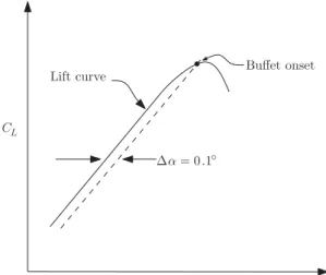
A number of techniques have been developed over the years to correlate data, typically from wind-tunnel experiments, with buffet predictions from a flight-testing program. These techniques include correlations with the RMS signals from wind-tunnel model strain gauges, trailing-edge pressure divergence, axial force break, pitching moment break, and lift curve break [61,62]. The last two methods may be employed in numerical predictions by using CFD to integrate force and moment values. One way to implement the lift curve-break method is theΔα0.1method [63]. Using this method, the linear portion of the lift curve is offset to the right by 0.1 deg. The intersection of this line with the actual lift curve is used to estimate the buffet-onset point, as illustrated in Fig. 1. We could use this method to develop a buffet-onset constraint function but, in using global aerodynamic coefficients, such asCLandCM, we would not make full use of the detailed flow solution provided by CFD. In addition, the“linear”portion of the lift curve slope is not exactly linear in

transonic flow, and identifying the slope to be used introduces ambiguity. The use of this approach with CFD requires at least two additional flow solutions (one for the slope, and one for the intersection). Finally, implementing a constraint based on this method would provide the optimizer with the opportunity to artificially affect the buffet onset by manipulating the lift curve at lower lift coefficients.

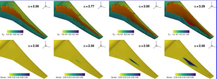
To develop a more direct way of constraining buffet onset, we focus on the physical mechanism of shock-induced flow separation, which is responsible for the loss of lift and the subsequent lowering of the lift curve slope. An example showing the typical progression of this type of separation with increasing angle of attack is shown in Fig. 2. To obtain the results shown in this figure, we performed a series of RANS solutions for the full Common Research Model (CRM) aircraft configuration (wing, fuselage, and horizontal tail), which is the same geometry that was used in the Fourth Drag Prediction Workshop [64], and it is representative of a long-range transport aircraft. The first row in Fig. 2 shows the friction lines and pressure coefficient, as well as the Lovely–Haimes shock sensor (in orange) [65].

To determine if the flow is separated at a given location on the surface, we check if the surface flow velocity has a component in the negative freestream direction (which is approximately the negative

x-axis direction), i.e., if

cosθ V⋅V∞

jVjjV∞j<0 (1)

where θ is the angle between the local surface velocity and the freestream. We can then define a separation sensor as

χ

1 if cosθ≤0

0 if cosθ>0 (2)

Thus,χ is specific to each surface location and is a Heaviside function: It is equal to one when the flow is separated, and it is equal to zero when the flow is attached. The blue areas on the surface for

α3.00 degandα3.29 degin the bottom row of Fig. 2 show the regions whereχ1, which approximately coincide with the regions where the flow is separated.

Our hypothesis is that the value of the area whereχ1correlates with buffet onset, which is given by the integral ofχover the whole surface area of the wing. Because we need to use this function as a constraint in a gradient-based optimization, we would like this function to be smooth. However, because this integral will be discretized based on a CFD surface mesh, andχis either zero or one for a given cell, the value of this area does not change continuously with the design variables. To address this issue, we use a smooth Heaviside function to blend the discontinuity as follows:

χ 1

1e2kcosθλ (3)

In this equation,kandλare free parameters, wherekdetermines the sharpness of the transition andλis a parameter that can be used to shift the smoothing function to the left or right as a function of the angle. For our cell-centered solver, the values forVare taken from the state variables at the cell center immediately adjacent to the wall because the velocities at the wall are zero when enforcing the no-slip condition. Figure 3 shows smooth Heaviside functions forλ−0.1, to 0, and 1; andk10. A value ofk10is used for all results in this paper. The bottom row of Fig. 2 shows the value of the smoothed separation sensor [Eq. (4)] on the wing surface atM0.85. The smooth Heaviside function smoothes outVxaround the separated

flow region. This area formulation can also be applied to constrain other undesirable phenomena, including cavitation [46,66].

Next, we can integrate the smooth separation sensor [Eq. (3)] over the surface and normalize it by the aircraft reference area to obtain the proposed separation metric:

Fig. 1 Estimating the buffet boundary with theΔα0.1method.

Ssep 1 Sref Z S χdS (4)

This is equivalent to performing a weighted area integration of the sensor value shown in the bottom row of Fig. 2.

To find out if the separation metric [Eq. (4)] is correlated to buffet onset, we use theΔα0.1method as a reference. We start by using the Δα0.1 method to compute the buffet boundary for the baseline CRM configuration [64] at a flight altitude of 37,000 ft and for Mach numbers ranging from 0.8 to 0.9. The resulting reference buffet boundary is shown as the orange line in Fig. 4 (Δα0.1

method). We then plot the lines corresponding to various values of the separation metric, and we determine that a cutoff value of

χ4%yields the best agreement when compared with theΔα

0.1method.

The overall shape of the buffet onset is consistent with the separation-based criteria, although some discrepancy exists. The discrepancy can be explained by analyzing the slopes of the lift curves for the baseline configuration, which we plot in Fig. 5. The figure also shows the application of theΔα0.1method, where the line slopes are based on the first two analysis points at the lowestCL

values for each Mach number. The lift curves are close to linear, but the slope of the lift curve increases for Mach numbers in the range 0.81–0.86. Therefore, at these Mach numbers, theΔα0.1method

overpredicts buffet onset compared with the separation-based method because the slope of the lift curve must decrease more to intersect the offset line. For Mach numbers greater than 0.86, the opposite effect occurs: The lift curves exhibit a reduced slope and intersect the linear offset at lowerCL values, underpredicting the

buffet onset. The differences in Fig. 4 are consistent with this effect. As we can see, the separation-based approach varies more smoothly

Fig. 2 Progression of separated flow for the CRM configuration atM0.85with increasing angle of attack. Top row shows the surface streamlines and pressure coefficient, as well as the reversed flow (red) and the shock (orange). Bottom row shows the value of the separation area integrand from Eq. (4).

0 30 60 90 120 150 180 0 0.5 1 λ= -0.1 λ= 0 θ (°) χ λ= 0.1

Fig. 3 Smoothed separation sensor value [Eq. (3)] versus angle of surface flow. Withk10, the smooth transition occurs over15 deg.

3% cutoff 2% cutoff Mach CL 0.8 0.82 0.84 0.86 0.88 0.9 0.3 0.35 0.4 0.45 0.5 0.55 0.6 0.65 0.7 0.75 0.8 Δα= 0.1 method Separation (_λ= -0.1, 4% cutoff)

Fig. 4 Results of the Δα0.1method compared with those of the proposed separation-metric method.

CL 0.2 0.3 0.4 0.5 0.6 0.7 0.8 0.9 Mach: 0.805 0.82 0.835 0.85 0.865 0.88 0.895 2o Δα

Fig. 5 Baseline configuration lift curves andΔα0.1linear offset for Mach 0.8–0.9. Successive lift curves are offset by 0.5 deg.

with respect to Mach number, which is beneficial for gradient-based design optimization. Because the separation-based approach is more representative of the actual physics, we believe that it is the more accurate of the two methods.

Figure 6 shows how the separation-metric approach is used to construct the buffet-onset boundary. For eachαsweep at a fixed Mach number, the intersection of the separation curve with the specified cutoff value determines the boundary. With nearly fully attached flow on the wing upper surface, the sensor metric is close to zero. Next, as α increases, the sensor metric rapidly increases as shock-induced flow separation becomes more severe. The large slope of the separation sensor curve means that theCL

value predicted for buffet is not particularly sensitive to the selected cutoff value.

To validate the proposed separation metric as a way to constrain buffet-onset, we compare the results obtained by using this approach with the experimental results by Balakrishna and Acheson [67], who tested the CRM wind-tunnel model. They estimated the buffet onset by making high-speed measurements of the strain at the wing root. Buffet onset can be identified by the increase in the strain-gauge signal amplitude, which is caused by the shock oscillations

interacting with the separated flow. Based on this increase in signal amplitude, they defined the buffet coefficientCB.

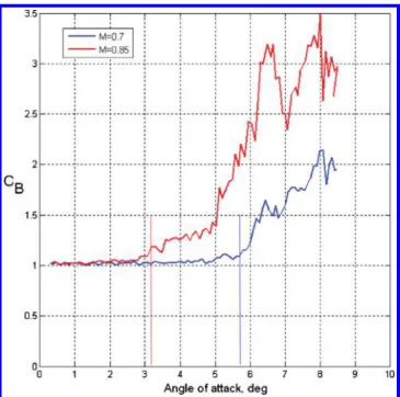
Figure 7, which is reproduced from figure 4 in the work of Balakrishna and Acheson [67], shows the evolution of the buffet coefficient for two Mach numbers: a high subsonic Mach number (M0.70), and a transonic Mach number (M0.85). We overlay lines atαvalues, for which our method yields a separation sensor value of 4%, withλ−0.1. We see that the results of the separation sensor method correlate well with the increase inCB, providing more

evidence that the separation-metric approach correctly predicts buffet onset.

Figure 8 shows the surface distribution ofCpand the smoothed

separation sensor for the two flow conditions. Due to the differing freestream Mach numbers, the types of separation and the corresponding separation locations are different. For theM0.70

case, a separation bubble appears just aft of the small leading-edge sonic region, whereas for theM0.85case, the separated flow appears near the midchord position at the foot of a strong normal shock. Although more comparisons with experimental results are required, the separation sensor adequately predicts buffet onset at both high subsonic and transonic flow conditions for this aircraft geometry.

IV. Full-Configuration Aerodynamic Shape Optimization Benchmark

We now demonstrate the need to consider buffet-onset criteria and the effectiveness of the proposed approach for transonic aerodynamic shape optimization by solving a series of aerodynamic design optimization problems based on the AIAA ADODG Case 5 benchmark [21].

A. Baseline Geometry

The baseline geometry defined in ADODG Case 5 is taken directly from the Fourth Drag Prediction Workshop’s “wing–body–tail

iH0”aircraft configuration [68]. This configuration is known as

the Common Research Model and is representative of a twin-aisle long-range transport. The main reference parameters for the CRM are listed in Table 1.

B. Computational Meshes

We generated a sequence of four CFD meshes for the CRM wing– body–tail configuration using the meshing software ICEM CFD. The meshes are divided into two families: the“1 series”and the“0.5 series.”Each 0.5-series mesh has approximately 2.5 times more cells than the corresponding coarser 1-series mesh below it and has approximately 3.3 times fewer cells than the next finer 1-series mesh above it. The two coarsest grids (L2 and L1.5) are used for optimization, whereas the two finest grids (L1 and L0.5) are used only for postoptimization verification purposes. The mesh metrics are summarized in Table 2. Figure 9 compares the surface mesh resolution of the four meshes. Grid-convergence studies for the baseline mesh and all optimized configuration meshes are presented in Sec. V.C.

C. Optimization Problem Statement

A sequence of seven design optimizations are solved to study the aerodynamic shape optimization of the ADODG full CRM configuration, as well as to demonstrate the effectiveness of the proposed approach for satisfying buffet requirements. These cases, numbered 5.1 through 5.7, are summarized in Table 3. Only cases 5.1 and 5.2 are currently specified by the ADODG [21]. We added the other cases (cases 5.3 through 5.7) to further study the effects of including buffet-onset conditions on the optimized geometries. The objective of all optimizations (except for case 5.7, which is discussed separately) is to reduce the weighted drag coefficient at the N

operating conditions. The optimization problem statement is summarized in Table 4.

Each flight conditioniis assigned a weightWithat specifies to

what extent the drag of the given flight condition influences the CL S e pa ra tion ( % ) 0.2 0.3 0.4 0.5 0.6 0.7 0.8 0 1 2 3 4 5 6 7 Mach: 0.8 0.82 0.84 0.86 0.88 0.9 Increasing α Cutoff=4% Baseline

Fig. 6 Separation sensor curves forαsweeps and for a range of Mach numbers. The cutoff value indicates the estimated buffet boundary.

Fig. 7 Buffet coefficient CB obtained from wind-tunnel data [67]. Vertical lines are the buffet-onset locations predicted by the separation sensor.

objective function. The lift and moment coefficient constraints ensure that the aircraft is trimmed at each flight condition, which can be achieved by the appropriate combination of angle of attack and tail rotation angle. The thicknesstjis computed at 750 points arranged in a25×30 regular grid in the chordwise and spanwise directions, respectively. These thicknesses are constrained to be greater than or equal to the original thicknesses of the CRM geometry at the corresponding points. Because making the wing as thin as possible is desirable in transonic flow [14], these constraints ensure that the wing does not become too thin, which would result in a significant increase

in structural weight. Imposing thickness constraints means that only changes in the wing camber are available to the optimizer.

Only cases 5.4, 5.5, and 5.7 use the separation constraint to satisfy the buffet margin. In these cases, the separation constraint is only enforced for the last two flight conditions, and the drag coefficient for these conditions does not contribute to the objective function (i.e., Wi0). Therefore, the adjoint for CD is not

evaluated for the buffet-onset conditions. Conversely, the separation-metric adjoint is not evaluated for the conditions where the drag coefficient weights are nonzero. This results in a total of three adjoint solutions being required for both the cruise and buffet flight conditions, which is desirable from a computational load-balancing perspective.

The ADODG specification for Case 5 disallows the parameter-ization from modifying the planform, and any shape modification may only be made in the vertical direction. Additionally, twist rotation is permitted for the wing, as is a solid-body rotation of the horizontal tail for trimming the aircraft. We use the FFD approach described in Sec. II.C. The FFD volume and the associated geometric design variables are shown in Fig. 10.

V. Results A. Multilevel Approach

To reduce the overall computational cost of performing the optimizations, we employ the multilevel optimization approach described previously by Lyu et al. [12] and the authors [14]. Optimizations are first carried out on the coarsest mesh (L2), the resulting optimum design becomes the starting design for the next finer mesh (L1.5), and so on. In this work, only the first two grid levels are used for the optimization. Because optimizing on the coarse grid costs less, we can afford to do more iterations on this grid. For

Fig. 8 Cpand smoothed separation sensor surface distribution for the two experimental buffet-onset conditions. In both cases, the separation (red) appears behind the shock (orange).

Table 1 Reference quantities for CRM full configuration [68]

Quantity Value

Reference area 594;720.0 in:2

Reference chord 275.8 in. Moment reference (1325.90, 0, 177.95) in. Reynolds number (M0.85) 43×106

Table 2 Mesh characteristics and corresponding trimmed drag coefficient for baseline configuration

Mesh level

Chordwise cells

Spanwise

cells ymax Total cells

BaselineCD (counts) L0.5 224 144 ∼0.5 14,233,600 231.15 L1 168 108 ∼0.7 5,921,536 234.87 L1.5 112 72 ∼1.1 1,779,200 249.47 L2 84 54 ∼1.7 740,192 269.76

Fig. 9 Spatial resolution for each mesh size.

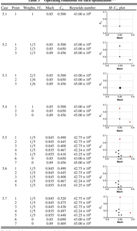
Table 3 Operating conditions for each optimizationa,b,c

Case Point Weights,Wi Mach CL Reynolds number M–CLplot

5.1 1 1 0.85 0.500 43.00×106 Mach CL 0.8 0.85 0.9 0.4 0.5 0.6 0.7 5.2 1 1∕3 0.85 0.500 43.00×106 Mach CL 0.8 0.85 0.9 0.4 0.5 0.6 0.7 2 1∕3 0.85 0.650 43.00×106 3 1∕3 0.89 0.456 45.00×106 5.3 1 2∕3 0.85 0.500 43.00×106 Mach CL 0.8 0.85 0.9 0.4 0.5 0.6 0.7 2 1∕6 0.85 0.650 43.00×106 3 1∕6 0.89 0.456 45.00×106 5.4 1 1 0.85 0.500 43.00×106 Mach CL 0.8 0.85 0.9 0.4 0.5 0.6 0.7 2 0 0.85 0.650 43.00×106 3 0 0.89 0.456 45.00×106 5.5 1 1∕5 0.845 0.490 42.75×106 Mach CL 0.8 0.85 0.9 0.4 0.5 0.6 0.7 2 1∕5 0.845 0.445 42.75×106 3 1∕5 0.845 0.408 42.75×106 4 1∕5 0.835 0.467 42.24×106 5 1∕5 0.855 0.418 43.25×106 6 0 0.85 0.650 43.00×106 7 0 0.89 0.456 45.00×106 5.6 1 1∕5 0.845 0.490 42.75×106 Mach CL 0.8 0.85 0.9 0.4 0.5 0.6 0.7 2 1∕5 0.845 0.445 42.75×106 3 1∕5 0.845 0.408 42.75×106 4 1∕5 0.835 0.467 42.24×106 5 1∕5 0.855 0.418 43.25×106 5.7 1 1∕5 0.845 0.520 42.75×106 Mach CL 0.8 0.85 0.9 0.4 0.5 0.6 0.7 2 1∕5 0.845 0.475 42.75×106 3 1∕5 0.845 0.438 42.75×106 4 1∕5 0.835 0.497 42.24×106 5 1∕5 0.855 0.448 43.25×106 6 0 0.85 0.690 43.00×106 7 0 0.89 0.469 45.00×106

a_{Red diamonds denote separation-constrained points.}

b_{Operating conditions for Case 5.7 are determined by the optimization process itself.} c_{Zero weight means that only the flight condition is considered for the constraints.}

this approach to be effective, the coarse grid must capture the main characteristics of the flow.

Figure 11 compares the baseline and optimized designs for Case 5.1. The aircraft planform views show the baseline and optimized designs obtained by using the L2 grid and the L1.5 optimization obtained by using the L2 optimized shape as the starting point. Color-coded slices of the airfoil shapes and the correspondingCp

distributions are shown for four spanwise locations at the bottom of the figure. We see that the coarse optimization (using the L2 grid) successfully eliminates the shock on the upper wing surface, resulting in parallel isobars. Even without further optimization, almost all of the drag improvement predicted by the coarse grid is realized on the fine grid. A comparison of the orange and black lines on the outer Cp distributions shows that the only significant

difference is the appearance of a weak shock on the refined grid. The fine optimization further improves the design, eliminating this shock and lowering the drag even further. This behavior is consistent with previous results, where three uniformly refined grid levels were used [12]. We employ this multilevel approach for all optimizations in the present work.

B. Optimization Results

In this section, we present the main results for each CRM aerodynamic shape optimization (cases 5.1 through 5.7). Figure 12 shows the evolution of the SNOPT merit function and optimality. The merit function is the value of the augmented Lagrangian given by SNOPT, which becomes the same as the objective function value once all the constraints are satisfied toward the end of the optimizations. The optimality is the residual of the Karush–Kuhn– Tucker optimality conditions, which measure how well the optimization has converged [57].

Fig. 10 CRM configuration showing the design variables for shape, twist, and tail rotation.

Table 4 Design optimization problem statement forNflight conditions

Function/variable Quantity minimize PN

i1WiCDi

with respect to airfoil shape variables 216

wing twist 9

angle of attack,αi N

tail rotation angle,ηi N

subject to CLi−C Li0.0 N CM_yi0.0 N tj≥tjCRM 750 Ssepi≤0.04 N

Fig. 11 Baseline design compared with optimized designs for Case 5.1. The coarse-grid optimum is a good starting point for the fine-grid optimization.

The optimality tolerance was set to10−5_{, which is achieved for}

most optimizations. The L2 optimizations are limited to 150 iterations, whereas the L1.5 optimizations are limited to a further 50 iterations. Case 5.7 uses a different objective function and is a maximization instead of a minimization. Generally, the finer optimizations with the L1.5 mesh achieved the same convergence tolerance as the coarse L2 mesh.

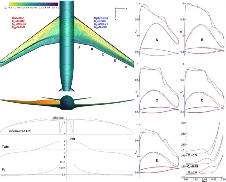
Figures 13 and 14 summarize the key features of the two ADODG optimizations (cases 5.1 and 5.2, respectively). The results of the baseline configuration are shown in red, and the optimized results are shown in blue. The planform view of the wing and fuselage shows the

Cp contours of the baseline geometry (left) and the optimized

geometry (right) under the nominal operating conditions (M0.85,

CL0.5). Just below the planform view, the front view also shows

theCpcontours and adds a visualization of the shock surface [65].

Below the front view, we plot the spanwise distributions of the lift, twist, and thickness-to-chord ratio (t∕c). A reference elliptic lift distribution is shown in gray. The right side of the figure displays the cross-sectional shapes and Cp distributions at the five spanwise locations indicated by the labels A–E in the planform view. Finally, the bottom-right plot shows the drag divergence behavior for three lift coefficients:CL 0.45;0.50;0.55.

The single-point optimization (Case 5.1) is similar to the wing-alone optimization done in previous work [12], where it was referred to as“aerodynamic shape optimization without thickness reduction.” In that case, the wing-alone configuration was optimized at the same Mach number and lift coefficient but at a much lower wind-tunnel Reynolds number of5×106_{. The previous work indicated that a 10.5}

drag count reduction was possible for the CRM wing-alone configuration. This compares well with the 8.6 count reduction that we obtain in the full wing–body–tail configuration studied herein. The cross-sectional plots of the airfoils at various spanwise sections show how little the shape needs to be modified to obtain a substantial change in performance. The drag divergence curves highlight the single-point design nature of the optimized configuration. A drag dip is present at the ondesign condition, but the performance is worse at most other Mach numbers and lift coefficients.

When we introduced theα0.1method previously for predicting buffet onset, we showed the lift curves for the baseline configuration

in Fig. 5. We now compute the same curves for the optimized configuration of Case 5.1, as shown in Fig. 15. The deviation from the linear slope observed in the baseline is more pronounced for this optimized aircraft, which means that including a physics-based buffet-onset constraint as we propose is all the more crucial; otherwise, the optimizer would exploit the lack of such a constraint and produce designs that are not realizable.

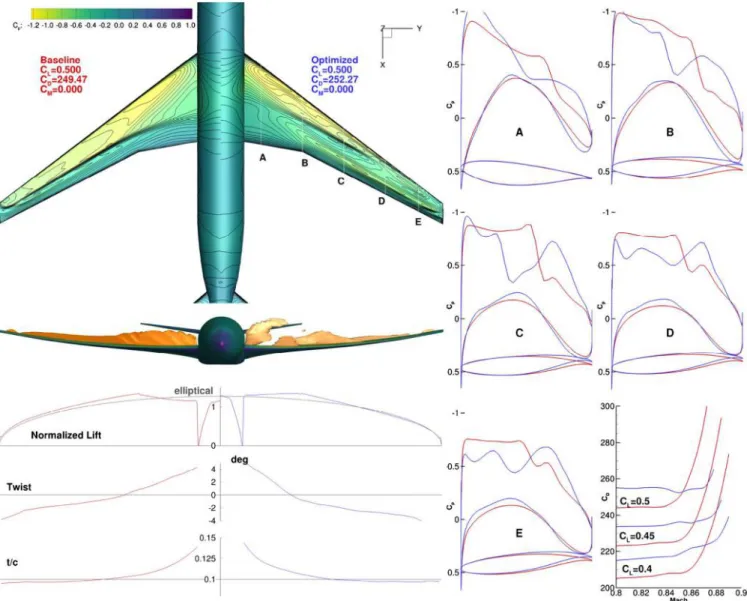
Case 5.2 adds two additional equally weighted operating conditions near the buffet-onset boundary. Unlike Case 5.1, for which we obtain a shock-free wing, Case 5.2 results in double shocks at the nominal operating condition. In this case, the drag at the nominal operating condition actually increases by 2.8 counts, as shown in Fig. 14. The drag divergence curves indicate a significant drag penalty across the lower Mach numbers, but this design does have a much higher drag divergence Mach number than the baseline design.

Although drag coefficient divergence curves yield useful insights into optimized designs, examining the performance in the fullM–CL

space is particularly instructive. In the context of transonic transport wing design,ML∕Dis a better measure of performance because it includes the benefit imparted on overall aircraft efficiency by a higher cruise speed. This overall performance can be approximated by the Breguet range equation

RMa c L Dln W1 W2 (5)

whereL∕Dis the lift-to-drag ratio;ais the speed of sound;cis the thrust-specific fuel consumption; andW1andW2are the initial and

final cruise weights, respectively. For a purely aerodynamic optimization at a fixed Mach number, onlyL∕Dvaries if we assume a constantcand weight ratioW1∕W2, so we are left withML∕D.

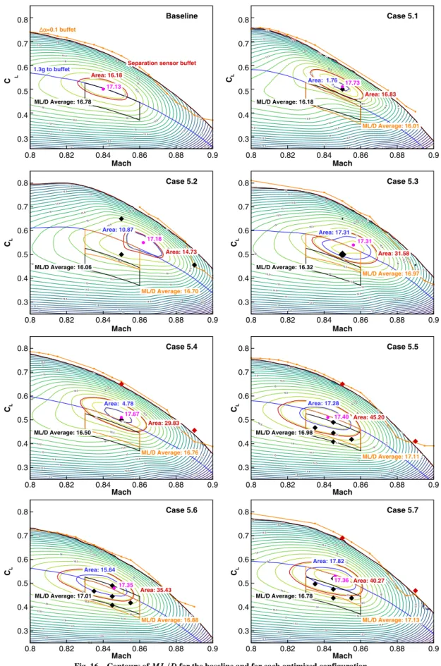
The procedure for generating contour plots is detailed in the Appendix. The contour plots are generated by using the L1.5 grid, and we ignore the additional drag associated with the nacelle, pylon, and vertical stabilizer. Figure 16 shows contour plots for all seven optimizations and the baseline design.

Iteration Optimality 0 50 100 150 10-5 10-4 10-3 Merit function 0.0225 0.0235 0.0245 0.0255 0.0265 0.0275 L2 L1.5 Case 5.1 Merit function 0.0225 0.0235 0.0245 0.0255 0.0265 0.0275 L2 L1.5 Case 5.4 Iteration Optimality 0 50 100 150 10-5 10-4 10-3 10-2 Merit function 0.03 0.032 0.034 0.036 0.038 L2 L1.5 Case 5.2 Iteration Optimality 0 50 100 150 10-5 10-4 10-3 Merit function 0.022 0.023 0.024 0.025 0.026 0.027 L2 L1.5 Case 5.5 Iteration Optimality 0 50 100 150 10-5 10-4 10-3 10-2 Merit function 0.027 0.028 0.029 0.03 0.031 L2 L1.5 Case 5.3 Merit function 0.02 0.025 0.03 L2 L1.5 Case 5.6 Iteration Optimality 0 50 100 150 10-5 10-4 10-3 10-2 Iteration Optimality 0 50 100 150 10-5 10-4 10-3 10-2 Merit function 15 16 17 18 L2 L1 Case 5.7 Iteration Optimality 0 50 100 150 10-3 10-2 10-1 100

Fig. 12 Merit function and optimality evolution for each optimization case.

The contours in each figure extend up to the predicted buffet-onset curve shown in red. The orange curve shows the buffet onset predicted by using the Δα0.1 method described in Sec. III. Several regions appear where the orange curves are missing data, which we attribute to the failure to find an intersection between the two lift curves. Overall, the separation-metric method continues to produce results that are close to those of theΔα0.1method, despite the large changes in the buffet-onset boundary.

The blue curve represents the 30% margin to buffet-onset boundary and is computed directly from the red buffet-onset curve. For normal operation, only operating conditions below the buffet-margin curve can be considered. The absolute maximum ML∕D

value for each configuration is shown in pink. Two specific contours for the optimization configuration (one for the baseline configuration) are highlighted: the contour of 99%ML∕Dmaxfor

the particular design is shown in blue, and the contour of 99%

ML∕Dmax for the baseline configuration are shown in red. The

motivation for plotting these 99% contours is that airliners typically fly between the Mach number yielding maximum range (approximated by the maximumML∕Dvalue in the figures) and a higher Mach number that yields a 1% fuel-burn penalty but decreases in the flight time. The area enclosed by both of these contours is used to quantify the robustness of the design in these figures. The areas are scaled by a factor of1002_{so that the area of the rectangle measuring}

0.01 inMand 0.01 inCLhas unit area.

The design operating conditions listed in Table 3 are shown as diamonds. The operating conditions considered for the objective function are shown in black, whereas the buffet-onset constraint

conditions are shown in red. The first buffet point (M0.85,

CL0.65) is at the nominal cruise Mach number and theCLvalue

corresponding to a 1.3g maneuver. The second buffet point (M0.89,CL0.456) is 0.04 higher in Mach number, which is a

typical margin between a nominal cruise Mach number and the maximum Mach numberMMOcondition. The lift coefficient for this

condition is adjusted to give the same dimensional lift as the nominal cruise condition at the same altitude.

Two additional regions are highlighted in black and orange, which we refer to as integration regions. They are constructed as follows: The Mach range is from 0.83 to 0.86, which corresponds to the typical range of operating Mach numbers for an aircraft such as the CRM. The upper line corresponds to the buffet-margin boundary, which is equivalent to specifying the maximum altitude the aircraft can fly for a particular weight. The bottom line corresponds to the reducedCLfor a 4000 ft decrease in altitude. To put it in another way,

the integration region contains all operating conditions within 4000 ft of the buffet-constrained ceiling and for all normal operating Mach numbers. The aircraft spends the vast majority of cruising flight in this region. The black integration region corresponds to the baseline design, whereas the orange regions are adjusted to reflect the actual buffet-margin boundary for each design. In addition, the upper edge of the black region indicates how the buffet-onset boundary changes for each design relative to the baseline configuration for the specific Mach range of integration.

Figure 17 displays a different visualization of the data already shown in Fig. 16. Here, we plot the percent change of each design relative to the baseline configuration. Note that the plot region is

Fig. 13 Baseline analysis compared to the Case 5.1 result. This single-point optimization leads to high performance at the nominal operating condition.

limited to flight conditions below the buffet boundary corresponding to each design. The color of the boundary indicates which is one active: The black boundary indicates the baseline buffet boundary is active, meaning that the optimized design boundary is higher than the baseline. The orange boundary means that the optimized boundary is active, and thus lower than the baseline buffet boundary. The integration region for each configuration is also shown in orange.

The contour plots give a much more complete understanding of the optimized designs. Unsurprisingly, the single-point optimiza-tion (Case 5.1) produces the highestML∕Dvalue, which is almost exactly matched to the design operating condition. However, with no way to constrain the buffet-onset boundary, the value of

ML∕Dmax is now above the buffet-margin boundary, which

means that this high-performance point cannot be achieved in practice because it falls outside the normal flight envelope. The 99%

ML∕Dmaxcontour (blue) is small, indicating a highly localized

point design. Despite the highML∕Dvalue, the averageML∕Din its own integration region (orange) is 4.6% worse than that for the baseline design.

For Case 5.2, the addition of operating conditions at the edge of the buffet-onset envelope substantially improves the buffet boundary over the entire range of Mach numbers. This case results in the most robust buffet-onset behavior of all cases. However, the value of

ML∕Dmaxbarely improves over that of the baseline design (17.18

vs 17.13). Worse still, as in Case 5.1, the high-performance region lies almost entirely outside the buffet-margin boundary, rendering the high-performance region unattainable. Even for this case, the average

ML∕Din the integration region is slightly worse (−0.5%) than for the baseline design. Note that the increased performance afforded by the higher buffet boundary is only possible if the baseline aircraft is buffet limited in altitude over the specific range of Mach numbers, as opposed to thrust limited. If the aircraft were thrust limited over the integration range, the obtainable performance would be the integral over the black integration region.

Fig. 14 Baseline analysis compared to the Case 5.2 result. To obtain a small improvement at the highest Mach numbers, performance is sacrificed across a large range of Mach numbers.

CL 0.2 Δα 0.3 0.4 0.5 0.6 0.7 0.8 0.9 Mach: 0.805 0.82 0.835 0.85 0.865 0.88 0.895 2o

Fig. 15 Lift curves for the Case 5.1 configuration with successive lift curves offset by 0.5 deg. The lift curves for the optimized configuration are more nonlinear.

In Case 5.3, we attempt to improve upon Case 5.2 by reducing the weighting factor for the near-buffet conditions. For this case, the nominal operating condition has a weight of 2/3, whereas the remaining two points each have weights of 1/6. The adjusted weightings yield a much more useful design. This is the first case where a significant portion of the 99%ML∕Dmax contour falls

within the integration region. In addition, the design is robust, as evidenced by the larger area enclosed by the blue contour when compared to the baseline design. As with the two previous cases, the increased performance is only possible if the aircraft can operate at higher altitudes. The other problem with this case is that the specific weightings are picked arbitrarily. Although these particular

10 10.5 11 11 11.5 12 12.5 12.5 12.5 12.5 13 13 13.5 13.5 13.5 14 14 14 14 14.5 14.5 14 .5 14.5 15 15 15 15.5 1 5.5 15.5 15.5 16 16 16 16.5 16.5 17 1 7 17 .5 ML/D Average: 16.01 ML/D Average: 16.18 Area: 16.83 Area: 1.76 _17.73 Mach 0.8 0.82 0.84 0.86 0.88 0.9 0.3 0.4 0.5 0.6 0.7 0.8 Case 5.1 11.5 12 12 12 12.5 12.5 12.5 13 13 13 13.5 13.5 13 .5 13.5 14 14 14 14 14.5 14.5 14.5 14.5 14.5 15 15 15 15 15 15.5 15.5 1 5.5 15.5 15.5 16 16 16 16 16.5 16.5 16.5 17 17 ML/D Average: 16.06 ML/D Average: 16.70 Area: 14.73 Area: 10.87 17.18 Mach CL 0.8 0.82 0.84 0.86 0.88 0.9 0.3 0.4 0.5 0.6 0.7 0.8 Case 5.2 11.5 12 12.5 12.5 12.5 13 13 13 13.5 13.5 13.5 13.5 14 14 14 14 14.5 14.5 14.5 14.5 15 15 15 15 15 15.5 15.5 1_5.5 15.5 16 16 16 16 16.5 16.5 16.5 17 17 17.5 ML/D Average: 16.76 ML/D Average: 16.50 Area: 4.78 Area: 29.83 17.67 Mach CL 0.8 0.82 0.84 0.86 0.88 0.9 0.3 0.4 0.5 0.6 0.7 0.8 Case 5.4 11.5 12 12.5 12.5 13 13 13 13 13.5 13.5 13.5 14 14 14 14 14.5 14.5 1 4 .5 14.5 14 .5 15 15 1 5 15 15 15.5 15.5 15 .5 15.5 15.5 16 16 16 16 16 16.5 16 .5 16.5 17 17 ML/D Average: 16.32 ML/D Average: 16.97 Area: 17.31 Area: 31.58 17.31 Mach CL CL 0.8 0.82 0.84 0.86 0.88 0.9 0.3 0.4 0.5 0.6 0.7 0.8 Case 5.3 10.5 11 12 12.5 1 2 .5 13 13 13.5 13.5 14 14 14 14 14.5 14.5 14.5 14.5 14.5 15 15 15 15 15.5 15.5 15.5 15.5 16 16 16 16 16.5 16.5 16.5 1 7 ML/D Average: 16.78 Area: 16.18

1.3g to buffet Separation sensor buffet =0.1 buffet 17.13 Mach C L 0.8 0.82 0.84 0.86 0.88 0.9 0.3 0.4 0.5 0.6 0.7 0.8 Baseline 11 12 12.5 1 2.5 13 13 13.5 13.5 13.5 14 14 14 14 14.5 14.5 14 .5 14.5 15 15 15 15 15 15.5 1 5.5 15.5 15.5 16 16 16 16 16.5 16.5 16 .5 16.5 17 17 ML/D Average: 17.11 ML/D Average: 16.98 Area: 17.28 Area: 45.20 17.40 Mach CL 0.8 0.82 0.84 0.86 0.88 0.9 0.3 0.4 0.5 0.6 0.7 0.8 Case 5.5 10 11.5 12.5 12.5 13 13 1 3 13.5 13.5 14 14 1 4 14 14.5 14.5 14.5 15 15 15 15 15.5 15.5 15 .5 15.5 16 16 16 16 16.5 16.5 16.5 17 17 ML/D Average: 17.01 ML/D Average: 16.88 Area: 35.43 Area: 15.64 17.35 Mach CL 0.8 0.82 0.84 0.86 0.88 0.9 0.3 0.4 0.5 0.6 0.7 0.8 Case 5.6 10 10.5 11.5 12 12.5 12.5 12.5 13 13 1 3 13 13.5 13.5 1 3 .5 13.5 14 14 14 14.5 14.5 14.5 14.5 14.5 15 15 15 15 15 15.5 15.5 15.5 15.5 16 1 6 16 16 16.5 16.5 16.5 16.5 17 17 ML/D Average: 17.13 ML/D Average: 16.78 Area: 17.82 Area: 40.27 17.36 Mach CL 0.8 0.82 0.84 0.86 0.88 0.9 0.3 0.4 0.5 0.6 0.7 0.8 Case 5.7

Fig. 16 Contours ofML∕Dfor the baseline and for each optimized configuration.

weights yield acceptable results, these weight values are not guaranteed to work well for another configuration or optimization problem.

Case 5.4 is the first optimization to use the separation sensor directly as an optimization constraint. Case 5.4 retains the same operating conditions as cases 5.2 and 5.3 but, instead of having the drag from the

flight conditions near the buffet boundary contribute to the drag objective function, it uses the buffet-onset flight conditions to compute the separation sensor and constrain its value. Note that a slight discrepancy exists between the operating conditions (red diamonds) and the buffet-onset boundary itself. The reason for this result is that the buffet-onset conditions are analyzed by using the scalar Jameson–

Fig. 17 Percent difference inML∕Dbetween the baseline design and the optimized configuration.

Schmidt–Turkel dissipation scheme [69], which results in a solution with more dissipation than the matrix dissipation scheme. The scalar scheme provides the increased robustness necessary for the optimization, which is not necessary for the contour plot evaluations. The more dissipative scalar scheme slightly underpredicts the area of separated flow, so the buffet boundary in the contour plot is lower when analyzed with the matrix scheme for the contour plot. Overall, the performance of this design is similar to that obtained with single-point optimization (Case 5.1). Most of the high-performance region lies outside the integration region. However, the reduction in performance is not as pronounced as with Case 5.1, for which the performance is reduced by just 1.6% in the original integration region and by almost zero in the on-design integration region. Nevertheless, there is a small improvement in the buffet-onset boundary.

Upon analyzing the results from cases 5.1–5.4, we noticed that the nominal design point always appears toward the upper side, or even completely outside the integration region, and that all optimization discussed thus far fails to improve the performance in the baseline integration region. To address this issue, we formulate a multipoint optimization (Case 5.5). Previous optimizations performed by the authors on the CRM wing-alone configuration show that selecting five operating conditions arranged as a cross in theM–CL space

results in highly robust designs [14]. Because our goal is to improve the performance in the original integration region, we distribute the five conditions as follows. The nominal Mach number is reduced to 0.845 for the first three operating conditions. The first point lies on the1.3gbuffet-onset boundary, whereas the next two points are atCL

values corresponding to 2000 and 4000 ft below. The two remaining points are 2000 ft lower than the buffet-onset boundary with a variation in Mach number of0.01. The buffet-onset conditions are taken at M0.85, CL0.65, andM0.89, CL0.41. The

latter point is taken from the baseline design buffet-onset boundary. The overall performance of this case is superior to all previously discussed cases. The performance in the baseline integration region increases by 1.2%, and the performance of the updated integration region increases by 2.0%. The design is very robust, as shown by the area inside the 99%ML∕Dmaxcontour. Furthermore, the point of

maximum performance appears inside the operating envelope. Given these results, trying a lower nominalCLfor cases 5.2–5.4 may be worth considering in the future.

Next, we developed Case 5.6, which is designed to investigate the effect of removing the buffet-onset conditions present in Case 5.5. We wish to answer the following question: Is a multipoint optimization near the design operating condition sufficient to ensure a robust buffet-onset envelope? Unsurprisingly, without the buffet-buffet-onset constraints, the buffet-margin boundary drops slightly over the integration envelope, pushing the integration region into a lower-performance region. The average value ofML∕Dfor the integration region is 16.88, which is only 0.6% higher than for the baseline configuration and much smaller than the 2.0% improvement obtained in Case 5.5.

Finally, for Case 5.7, we formulate a different design optimization problem. We remove the requirement of specifying fixed design lift coefficients and let the optimization itself determine the ideal ondesign condition. All cases presented thus far are lift-constrained drag minimizations with fixed operating conditions. The fixed operating conditions also include fixing the value ofCL for the buffet-onset locations. In the formulation of Case 5.7, we want the optimization to directly adjust the single nominal operating condition. The remaining operating conditions are then explicitly linked to this designCL. More

specifically, the high-CLbuffet-onset conditions must have 1.35 times

the lift of the nominal cruise Mach. Although the minimum load factor is 1.3, to achieve a higher buffet-onset boundary for which more of the integration region lies inside the 99%ML∕Dmax contour, we use a

factor slightly greater than the minimum, hence the 1.35 value. The high-Mach buffet case must have the same physical lift as the nominal operating condition atM0.89and at the same altitude. Finally, the remaining operating conditions move vertically in sync with the changing design CL. The modified optimization formulation is

summarized in Table 5.

Note that the operating conditions (diamonds) shown in Fig. 16 are the optimized values. The optimization increased the nominal design

CLfrom the initial value of 0.490 (the value used in cases 5.5 and 5.6)

to 0.520. This increase is made possible by a corresponding increase in the buffet-onset boundary. The previous optimizations, especially Case 5.2, showed that there can be a significant penalty in cruise drag for a higher buffet boundary. For Case 5.7, we have given the optimizer sufficient information to make this tradeoff optimal. This results in a slightly higher average performance than Case 5.5 (17.13 vs 17.11), as well as a higher buffet-onset boundary. The design is also highly robust, exhibiting the largest 99%ML∕Dmaxcontour of

all the cases.

Further insight into the differences between the optimized designs is provided by Fig. 17. It is particularly interesting to see that there is a region betweenM0.86andM0.88at lowCLthat is universally

worse on all optimized designs. This is particularly noticeable on the single-point designs (cases 5.1 and 5.4). It is least evident in Case 5.5, where there is an improvement over almost the entire contour region. Compared to Case 5.7, the higher buffet-onset performance appears to be correlated with the reduced low-CL performance. The performance reduction at lower lift coefficients in Case 5.7 is limited to less than 2%, which is acceptable given the performance increase at the higher lift coefficients.

C. Grid Convergence

We studied grid convergence for the baseline geometry and for all optimized configurations. For the grid-convergence studies, we apply the optimized geometry from the L1.5 mesh to the each of the four meshes in sequence. The drag convergence for each mesh configuration is shown in Fig. 18. The drag coefficient, when plotted

Fig. 18 Grid-convergence study for baseline and all optimized configurations, showing that the change in drag is constant between grid levels.

Table 5 Design optimization problem statement forNflight conditions

Function/variable Quantity maximize PN

i1WiMiLi∕Di

with respect to airfoil shape variables 240

wing twist 9

angle of attack,αi N

tail rotation angle,ηi N

design,CL 1 subject to CLi−C Li0.0 N CM_yi0.0 N tj≥tjCRM 750 Ssepi≤0.04 N

against the grid factorN−_cells2∕3, is approximately linear, indicating second-order convergence. However, the finest mesh analyzed (L0.5) does not fall directly on the line, which indicates that a more highly resolved mesh is necessary to determine a grid-converged value. However, for aerodynamic shape optimization, we are generally more concerned with thechangein drag coefficient resulting from a design change as opposed to the grid-converged drag coefficient. Figure 19 shows the change in drag coefficient for each configuration on each mesh level. Remarkably little variation occurs across each mesh level, which we attribute to the fact that the spurious drag remains roughly constant for a given mesh, independent of the design modifications. The maximum variation between the improvement on the L1.5 mesh, which is the finest mesh used for optimization, and the L0.5 mesh is 0.63 counts (in Case 5.6). Given the much larger computational cost of optimizing with the L1 or L0.5 meshes and the small difference in predicted drag improvement when using these finer meshes, the use the L1.5 mesh for our optimizations is a good choice.

D. Computational Cost

Multipoint three-dimensional RANS-based aerodynamic shape optimizations are costly from a computational perspective, so we make every effort to reduce the total cost of the optimizations. Table 6 lists the total CPU cost, in processor hours, required to generate the results presented in this paper. All the computations were performed on nodes with two four-core E5540 CPUs running at 2.53 GHz with 16 GB of RAM per node. The nodes are connected with QDR InfiniBand [70]. All L2 and L1.5 meshes were run on 64 cores, whereas the L1 and L0.5 meshes for the grid-convergence study used 128 cores.

The optimization consumed 63% of the total computational time, and the remainder of the time was used for postprocessing. The

ML∕D contour plots were particularly costly because each plot required approximately 400–500 individual CFD evaluations.

VI. Conclusions

A new formulation for predicting buffet onset and for effectively implementing it as a design optimization constraint is presented. The proposed method is based on the integration of a separation sensor along with a cutoff value to estimate when buffet first occurs and can be directly evaluated with only one steady RANS CFD solution. The results of this method compare well with those of theΔα0.1

method for the CRM configuration, and for various optimized designs. A comparison with experimental data obtained from wind-tunnel tests also shows that the proposed model has good predictive capabilities. The separation sensor method is particularly well suited for formulating a constraint in gradient-based optimization because it is easy to implement in a discrete adjoint optimization framework, and the resulting function (although highly nonlinear) is smooth.

To demonstrate the effectiveness of the proposed approach, seven design optimization cases are solved starting from the CRM wing-body-tail baseline. All optimizations are done with respect to 216 shape variables; nine twist variables; and a tail rotation angle subject to lift, pitching moment, volume, thickness, and separation constraints. To reduce the overall computational cost, a two-level sequential optimization approach was applied. At the nominal operating condition of M0.85, CL0.5, the single-point optimization (Case 5.1) reduces the drag coefficient from 249.5 counts to 240.9 counts, which is a reduction of 3.4%. For a more complete comparison of the optimized designs, contours ofML∕D

were plotted inM–CLspace, which provided a visual and intuitive way of comparing the performance and robustness of the optimized configurations.

For Case 5.2, two operating conditions were added near buffet onset, which increased substantially the performance at these points and produced a high buffet-onset boundary. However, the overall performance as measured by a typical operating envelope was lower than the baseline. Although weighting the nominal cruise point (Case 5.3) more than the off-design condition improved performance, it required knowledge of how to choose the appropriate weights, which might be case dependent.

In Case 5.4, the use of the separation metric to directly control the buffet-onset and buffet-margin boundaries was introduced. Although this approach was effective, the overall performance of the optimized design was unsatisfactory; it was lower than that of the weighted-points approach in Case 5.3.

The remaining cases use five main operating conditions to produce more robust designs. The performance improves for Case 5.5 over nearly the entire transonic range, with a simultaneous improvement of part of the onset boundary. Case 5.6 removes the buffet-onset conditions, demonstrating the insufficiency of a multipoint optimization with all conditions near the ondesign condition. In this case, the buffet-margin boundary encroaches onto the cruise performance region, reducing the average usable improvement from 2.0% for Case 5.5 to only 0.6% for Case 5.6. Finally, in Case 5.7, a

ML∕Dmaximization was done with automatic determination of the operatingCL, which improved the average performance above that of

Case 5.5 while pushing the buffet-onset boundary beyond the operational envelope.

Given these results, it is recommended that physics-based buffet-onset constraints be enforced for aerodynamic and aerostructural shape optimization of transonic transports, as was done in this work. The separation metric developed herein is easily implemented and yields robust results, so it provides a much needed constraint formulation for the aerodynamic shape optimization community.

Appendix: Generation of Contour Plots

The generation of the contour plots shown in Fig. 16 warrants further explanation. These contours are not simpleαsweeps because Grid Factor

Δ

CD

0 2E-05 4E-05 6E-05 8E-05 0.0001 0.00012 0.00014 -12 -10 -8 -6 -4 -2 0 2 4 6

Fig. 19 Change in drag for the optimal designs relative to the baseline design, showing that this change is roughly constant for all designs between grid levels.

Table 6 Breakdown of computational cost in CPU hours

Case L2 optimization L1.5 optimization Contour Grid convergence Total Baseline — — 1,346 817 2,162 5.1 289 611 1,270 1,009 3,179 5.2 2,378 2,394 1,795 1,121 7,688 5.3 1,290 2,505 1,750 910 6,457 5.4 1,507 2,602 1,384 1,024 6,518 5.5 2,090 3,506 1,392 830 7,369 5.6 1,111 1,803 1,147 610 4,673 5.7 4,136 6,623 1,800 696 13,255 Total 12,802 19,567 11,886 7,019 51,303

the tail angle that givesCM0must be determined at each point. Once the flight condition in the contour is trimmed, the trim drag penalty is included in the computed drag coefficient. Naively performing a secant search to determine the tail angle at each point would require at least three CFD solutions. However, because each contour plot requires approximately 400 trim-converged solutions, we seek instead an alternative approach to reduce the computational cost to the extent possible.

One way to reduce the computational cost of producing these contours is to reuse previously evaluated points to continually update the2×2Jacobian of the residual,F CL−CL; CM, with respect

toα;η, whereαis the angle of attack andηis the tail rotation angle. With an accurate Jacobian, we can use Newton’s method to simultaneously determine the newα andη required to produce a trimmed solution at a new CL. The full procedure is listed in

Algorithm A2. An auxiliary function for computing the residual for a given (α,η) is given in Algorithm A1.

In practice, only one subiteration is necessary for most points because theCLandCMfunctions are not highly nonlinear functions of

α and η over most of the contour region. Generally, additional subiterations are only necessary as buffet is approached due to the more rapid variation in the lift curve slope. For example, the contour for the baseline configuration requires 430 function evaluations to produce 356 converged trimmed-CLsolutions, which is an increase of only 20%.

Note that we only check for the convergence ofCMbecause precisely

matching the lift coefficients to the specified target is not critical. Once all the raw data are generated, CL, CD, CM, and the

separation sensor values are interpolated by using an Akima spline [71] to produce a regularM–CLgrid. This regular grid is then used for further computations, such as the difference plots shown in Fig. 17 and the drag-divergence curves in Figs. 13 and 14, as well as for extracting particular contours and computing the average performance over specific integration regions.

Acknowledgments

Funding for this research was provided in part by NASA under grant number NNX11AI19A. The computations were performed in the Extreme Science and Engineering Discovery Environment,

Algorithm A2 Trimmed-C_Lcontour computation

1: Given:CLmin,M1; : : : ; MN,ΔC

L,α0,η0,Δα,Δη,Sepmax,Nsub,ϵ

2: SetMM1

3:F0Fα0;η0 T; CLmin

4:F1Fα0Δα;η0 T; CLmin

5:F2Fα0;η0ΔηT; CLmin

6:J F1−F0∕ΔαF2−F0∕Δη (Initial finite-difference Jacobian approximation)

7:JsaveJ

8:xsave α0;η0 T

9:fork←1; N,do (Loop overNsequential Mach numbers) 10: setMMk

11: JJsave (Restore Jacobian for lowestCL)

12: xnxsave (Restorexfor lowestCL)

13: ΔCLΔCL (Restore targetCLincrement)

14: CLCLmin (Set the targetCLto the lowest desiredCL)

15: FnFxn; CL (Evaluate current point)

16: continueTrue

17: i_α0

18: whilecontinue,do (αincrement loop)

19: forj←1,Nsub,do (Subiteration loop)

20: dxJ−1Fn (Newton’s method for update)

21: xn1xn−dx (New [α,η] solution)

22: Fn1Fxn1; CL (Solve CFD for the newx)

23: dFFn1−Fn

24: JJ dF−Jdx∕kdxk2_dxT _{(Update Jacobian using Broyden’s method)}

25: xnxn1 (Setxnfor next subiteration)

26: ifi_α0 (StoreJandxn1for the next Mach number on the lowestCL)

27: JsaveJ

28: xsavexn

29: end if

30: Evaluate separation sensor,Sep

31: ifSep>0.01then

32: ΔCL0.01 (Reduce the targetΔCLas buffet is approached)

33: end if

34: ifabs(Fn1) <ϵorjNsub,then (Only check convergence for moment)

35: CLCLΔCL (Update the next targetCL)

36: Fn Fn10−CL; Fn11] (Set the function value for the nextCL)

37: Break subiteration loop 38: else

39: FnFn1 (Continue to refine the current targetCL)

40: end if

41: end for

42: iαiα1

43: ifSep>Sepmax,then

44: continueFalse (Reached buffet onset, so proceed to next Mach number) 45: end if 46: end while 47:end for Algorithm A1 Trim-C_L function 1:functionFx; CL 2: Setαx0andηx1 3: Solve CFD problem 4:returnF CL−CL; CMT 5:end function