_____________________________________________________________________
CREDIT Research Paper
No. 09/11
_____________________________________________________________________
25 Years of Aid Allocation Practice:
Comparing Donors and Eras
by
Paul Clist
Abstract
Focusing on seven bilateral donors over a 25 year period, the paper answers 4 questions related to aid allocation practice. Questions one and two examine allocation differences between donors and time periods. Questions three and four relate to changes in poverty and policy selectivity. To answer these questions a formal approach is used to quantify the effects of four factors that influence aid allocation: poverty, policy, proximity and population. The results reaffirm findings of large donor heterogeneity and the role of non-development influences. However, they dispute recent findings of large or growing policy sensitivity.
JEL Classification: F35, F50,
Keywords: Aid Allocation, Policy Selectivity, Poverty Selectivity, Two-Part Model.
_____________________________________________________________________
Centre for Research in Economic Development and International Trade, University of Nottingham
_____________________________________________________________________
CREDIT Research Paper
No. 09/11
25 Years of Aid Allocation Practice:
Comparing Donors and Eras
by
Paul Clist
Outline 1. Introduction 2. Literature Review 3. Econometric Approach 4. Results 5. Discussion 6. Conclusion References Data Descriptions Appendix The AuthorsPaul Clist, School of Economics, University of Nottingham, Nottingham NG7 2RD, U.K. [email protected]
Acknowledgements
Comments from Oliver Morrissey, Alessia Isopi and Christopher Kirby are gratefully acknowledged.
_____________________________________________________________________ Research Papers at www.nottingham.ac.uk/economics/credit/
1.
Introduction
Both aid and its allocation have been much maligned in recent years. Criticism of the former has extended from econometric studies that fail to find a positive effect of aid on growth (see Roodman 2007 for a review), to more popular works that argue reductions in aid would promote development (Calderisi 2006;Glennie 2008;Moyo 2009). An obvious consequence of these critiques is to examine aid allocation itself. If aid is not found to promote development, is this an inherent feature of aid or the consequence of poor allocation practice by donors? Early research on Aid Allocation commonly proposed a dichotomy between donor interest and recipient need, and found the former dominated the later (e.g. McKinley and Little 1979), showing a possible source of distortion. However, there are three major reasons for thinking that aid allocation may have changed since that research was published. First, the end of the Cold War may have freed donors from security concerns to pursue a more development-centred allocation approach. Meernik et al. (1998, p.79) reported early evidence of an increased importance of poverty in allocation decisions in place of security concerns. In that same year it was reported policy-makers were still debating the proper role of aid in the post Cold War era (Schraeder, Hook, and Taylor 1998). Second, influential research (Burnside and Dollar 1998;2000) argued that aid worked in a good policy environment. The associated recommendation was that aid should change to reflect this conclusion, with a move from conditionality to policy selectivity (Collier and Dollar 2002). Third, the terrorist attacks of September the 11th 2001 in the USA saw large increases in American aid budgets and potentially large changes in allocation principles (Moss, Roodman, Standley, and Floor 2005).
In light of this, this research seeks to answer four questions. First, what are the donor differences? This is a static comparison of donor behaviour, to understand which factors guide which donors. In contrast with much of the literature, a formal approach is used to quantify differences between donors. This allows comparisons between donors, and between different factors that are thought to influence allocation practice. Second, what are the changes over time? As aforementioned, there is considerable reason to suspect general changes in allocation practice. Again, we employ a formal technique to identify any significant changes. The third and fourth questions are whether selectivity has
increase with relation to poverty and policy respectively. We employ different specifications in order to understand if the expected change has indeed occurred.
This research is both novel in technique and contribution to current debates. It applies an existing systematic approach to identifying differences in allocation behaviour between donors and over time within the more recent theoretical framework. This allows comparisons to be of a more formal nature. The econometric section includes an evaluation of the different techniques used and a strategy to test between them which are surprisingly atypical. This paper also corrects for the problems of serial correlation and aid volatility which are expected to be commonplace but seldom discussed. The salient contributions to our understanding of aid allocation are three fold. First, we are able to re-examine the effect of the end of the Cold War on allocation. Results suggest that early evidence for increased policy and poverty sensitivity are not easily replicated. Second, we find the evidence of a move from conditionality to selectivity doubtful. Third, the terrorist attacks of September 11th 2001 are shown to have had limited effect on aid allocation practice.
2
Literature Review
This research employs a positive approach and a small review of literature within that stream and directly relevant to the four questions proposed is included here.
Donor Differences
There has been surprisingly little attempt to formally test differences between donors, the common approach instead being a narrative description including some parameter differences. Berthélemy and Tichit (2004, pp.269-270) report the sign and significance level of the coefficients in their model for 18 bilateral donors. They find mixed evidence in support of the importance of recipient need, and find infant mortality to be a better predictor than income for many donors. Policy is significant for most donors, but the USA and Australia exhibit a special preference for democracy whereas France and Belgium both have a negative coefficient estimate. They do not report major differences in their Donor Interest variables, but state smaller donors focus regionally. Berthélemy (2006) divided donors into three categories on the basis of the estimated coefficient for the trade-aid relationship. Selfish donors (Australia, France, Italy, Japan and the UK)
have a positive relationship between aid and trade whereas Altruistic donors (Austria, Denmark, Ireland, Netherlands, Norway and Switzerland) have a negative relationship. Trade here is measured as the logged and lagged sum of imports and exports between the donor and recipient as a share of Donor’s GDP. Alesina and Dollar (2000) report that for 3 donors their allocation is distorted by a single factor: for the USA it is Israel and Egypt, for France it is colonies and for Japan it is UN voting records. They find France and Japan to be insensitive to Poverty whereas the USA and the Nordic countries give more to poor, democratic and open countries.
The most robust finding when comparing donors is that Nordic donors are distinct. Alesina and Weder (2002) focus on the link between corruption and aid allocation over the period 1975-1995, both in aggregate and by individual donors. Using the Tobit technique for individual donors, they find Nordic donors tend to give less to corrupt recipients, whereas for other donors there is no robust relationship. They postulated that Nordic donors are freed from colonial ties and can thus be more sensitive to other considerations. Gates and Hoeffler (2004) explicitly test and confirm the idea that Nordic donors (Norway, Denmark, Sweden and Finland) are different, finding them to be more influenced by democracy and less influenced by trade, compared with other donors.
Differences Over Time
When examining the differences in donor behaviour over time, the influence of the Cold War (CW, hereafter,) and 9/11 are particularly salient. Meernik et al. (1998, p.79) reported early evidence that the end of the cold war meant a declining importance of security concerns, a large drop in aid transfers in aggregate and an increased importance of poverty in allocation decisions. Boschini and Olofsgård (2007) concur that the CW may explain the decline in aid volumes, but argue that it changed relatively little in allocation practice. Berthélemy and Tichit (2004) argue that the geopolitical concerns of aid allocation during the CW have been replaced not by increased poverty concerns (which they actually find decrease) but by trade relationships. Easterly (2007) finds that the CW changed little in terms of sensitivity to democracy, and Neumayer (2003a) finds it had no effect on the relationship with human rights.
Moss et al. (2005) study the effect of Global War on Terror (GWOT) on US aid allocation using various variables thought to capture a priori expectations. They find that essentially the effect of the GWOT was to substantially increase the aid for four countries (Iraq, Afghanistan, Jordan and the Palestinian territories) which was financed mainly by an augmented aid budget but also by reductions for three countries (Israel, Egypt and Bosnia and Herzegovina). Fleck and Kilby (2009) find that the GWOT coincides with increased aid volumes for the USA, and that poverty sensitivity has decreased in this period. Others have tried to capture the effect of the GWOT simply by employing a dummy for the period. This is only a satisfactory modelling solution if the effect of the GWOT was a universal one time-shift in aid allocation transfers for all recipients. While the research implies the role of the GWOT is smaller than might have been expected for the US, this does not seem a suitable solution.
Poverty and Policy Selectivity
The empirical research that argued ‘aid works, with good policy’ quickly resulted in aid allocation principles (Collier and Dollar 2002) and, it is thought, into policy implementations (Easterly 2003). It would be expected that this would lead to a greater weight for policy in allocation decisions, but also a greater focus on poverty as aid is seen as a possible solution. This move from conditionality to selectivity was being discussed surprisingly early in policy circles (Hout 2007a), but it is unclear whether this move was rhetorical or actual. Hout (2007b) examines the allocations of the Netherlands, USA and World Bank and provides evidence that policy selectivity has not increased within the last few years. Looking at selectivity over a longer time horizon, Easterly (2007) finds increased poverty sensitivity to have happened after ‘the McNamara revolution’ of the 1970s, with little change since then. Regarding policy, he concludes that “The overall picture is that there is little evidence that donors are learning to be increasingly selective with respect to policies in the recipient countries.“ (ibid. p.654) Nunnenkamp and Thiele (2006) report correlations and basic regressions from a similar exercise in support of the conclusion that aid is poverty but not policy-sensitive. Specifically policy-insensitive are Japanese and French aid, with the US not fairing particularly well. The poverty focus is found particularly strong for Scandinavian countries, Germany, Holland and the UK.
In contrast to the aforementioned research, are two papers that claim policy selectivity has increased, specifically since the 1980s. Examining 22 bilateral donors over the period 1980-1999, Berthelemy and Tichit (2004, p267) find evidence of increasing selectivity: “… donors give more recognition for good economic policies in the 1990s than in the 1980s.” They use aid per capita as the dependent variable, arguing that this helps to examine the small-country bias, and a panel Tobit as the estimator, to capture fluctuations in the donor budget. The conclusion that aid allocation is more selective (in terms of economic policies) is based on the coefficient on lagged economic growth becoming positive and significant in the 1990s, whereas it was negative in the 1980s. FDI is also included in the specification: In the 1980s its coefficient was significant and positive, and in the 1990s it became insignificant and very small. Thus it is highly possible that the results are misleading, due to co-linearity. Leaving this aside, the use of lagged economic growth is highly problematic as a variable to capture ‘good economic policies’ for the following year. There are other potential explanations for aid ‘following’ growth that are as compelling as it signifying a concern for economic policy. For example, it may be desirable for a donor to be associated with a country that is growing relatively quickly. Alternatively, a selfish donor may use aid to promote its own exports, by allocating more aid to countries with an expanding market. Then again, it may be that donors imagine that a country with a recent growth record is able to absorb more investment in the form of aid, or conversely that countries that have experienced a negative shock (such as a natural disaster which led to an economic downturn) require higher aid commitments. In short, the evidence does not seem to fully justify the conclusion.
Dollar and Levin (2006) examine a large number of donors, both bilateral and multilateral. They estimate using a Tobit, with logged Aid disbursements as the dependent variable. They use two variables as proxies for policy: the International Country Risk Guide (ICRG) rule of law index and Freedom House’s democracy index, and GDP per capita data to inform conclusions on poverty sensitivity. They conclude, on the basis of their statistical analysis, that: “In the past two decades, foreign aid overall has become more selective [in terms of economic governance]” (ibid. p.2044) They find this increased selectivity is driven by multilateral agencies, whereas for bilateral donors economic governance has no statistically significant relationship with aid allocation. They
conclude that foreign aid overall is more selective in the early 00’s than in the late 80’s because more donors are significantly selective. However, this picture is highly misleading as in 2006 Multilateral Agencies represented only around 14% of all ODA commitments1. Aid donors may have become more selective on average, but has aid? This paper examines the strength of policy selectivity over the last twenty-five years, for the most important donors. By modelling only the most important donors, we hope to ascertain more closely the overall policy selectivity of aid. We thus hope to discover which set of papers reports the most robust result: Easterly (2007) and Nunnenkamp and Thiele (2006) who report static and low policy selectivity, or Dollar and Levin (2006) and Berthélemy and Tichit (2004) who report increasing policy selectivity.
3
Econometric Approach
The early dichotomy of recipient need and donor interest gave way to the hybrid model, where both factors had some influence over aid allocation, given by , . Instead of this model, we estimate the following by donor.
This is similar to Neumayer (2003), and hereafter referred to as a 4P specification. As in the RN-DI approach, Poverty describes the level of need in a potential recipient country. As poverty is thought to be a major motivation for aid, the a priori expectation is for this to be positive ( 0). Population is another standard variable, and expected to be positive ( 0). As discussed, Policy is a relatively recent addition to the theory of aid allocation and can be understood in a number of ways. Here it contains two main strands. The first is the ability of a recipient to turn a given amount of aid into a desirable outcome in the mind of the donor. This conceptualisation is similar to the normative proposal of Collier and Dollar (2002). The second aspect includes desirable characteristics of a donor that are not need-related, in the mind of a donor. For example, it may be argued that the USA value democracy inherently and for ideological reasons rather than any effect on poverty reduction. Both parts of policy would be expected to have a positive relationship with aid allocated ( 0).
Donor Interest was conceived as essentially incompatible with recipient need, a formulation still used (e.g. Berthélemy 2006, who uses the hybrid approach). In the original framework, Recipient Need and Donor Interest are mutually exclusive and a donor must choose between increasing their own welfare and that of recipients. Proximity
by contrast includes DI but can take many forms including religion, language, culture, history, geography and commerce. This wider understanding means factors that are less obviously in the direct interest of a donor can also be included. For example, it may be
altruistic for a donor to give to recipients if they share a common language if doing so
would decrease transaction costs and increase the value of aid. Indeed, given the critique of aid on the basis of fragmentation, it is perhaps the most sensible way for donors to choose which recipients to focus upon. Neither Poverty nor Policy change by donor but rather by recipient. If donors weight these factors in similar ways, there is no guidance of how to choose which recipients to focus upon. Instead, Proximity may suggest which recipients a donor should focus on, with possible efficiency gains due to lower linguistic or cultural barriers. Whether the motivation for allocations being influenced are good or ill, the expectation is that the relationship will be positive ( 0).
There has been surprisingly little work done which formalises the relative import of each factor on a donor’s aid allocation. Often the approach has been to ascribe levels of effect to specific variables, rather than the factor which may be represented by a number of variables. One exception to this is the work by McGillivray (2003, pp.8-9) on comparing DI and RN models, which is easily extended from RN-DI to the 4P setting (Hoeffler and Outram 2008). He argues that the fairest test between competing models is simply a joint test of significance on the group of variables representing that factor after a regression of the full model. This test is a test of the following as the null hypothesis, for all of the coefficients that represent the factor (e.g. for Proximity that might include variables for trade, colonial history and shared language):
: 0
The rationale of the test is to apportion explanatory power to the various competing hypotheses. Each may be significant, but at different levels. It is also informative when a
number of variables represent a single factor, as the test provides information on the factor level, not just the variable level. Having decided the general approach, there remain two main decisions: estimator and specification.
Which Estimator?
Data on aid flows are left-hand censored, i.e. many data points on aid transfers are zero. As such, OLS estimation would be biased, as the data is not normally distributed but instead clustered at the zero bound (see Figure 1). There are various estimators that can be used, which I will discuss these in turn, along with their assumptions and some relevant tests. For a more technical presentation of the estimators, see Cameron and Trivedi (2005, chp.16) or McGillivray (2003, with application to aid allocation).
Figure 1: OLS and Latent predictions of Aid Allocations
OLS
The simplest estimator, used recently in the aid allocation context by Alesina and Dollar (2000), is simply OLS. They use this estimator only when estimating ‘average donor performance’, and argue that the number of 0s is small enough for the bias to be of little consequence (Alesina and Dollar 2000, p.42). While this may be possible when the percentage of data censored is small, this is unlikely to be the case when estimating by donor. Figure 1 shows the predicted line when estimating using OLS, if all data are
included. The shaded dots show observed aid, whereas the hollow points show aid if it were allowed to be negative. The use of OLS then biases the predictions of beta toward zero, as the observed dependent variable understates the effect of the independent variables.
Censored Models
There are a number of different estimators that have been conceived with censoring in mind. Terminology is inconsistent in the literature, as the main authors use different names for the same estimator. Semantic broadening has further complicated matters, as Tobit is now often used to denote any parametric model that deals with censored data. Here we present 3 models that by that definition are Tobit models, each of which has been used to examine aid allocation behaviour in some form. Tests are presented alongside the estimator, and then the testing strategy is implemented. To briefly summarise, one major difference between the three types of Tobit is their assumption of the relationship between the two stages of the allocation process (eligibility and level). Tobit type 1 assumes each independent variable has the same effect in both the first and second stages. This allows the two stages to be estimated together, as if one were a continuation of the other. The Two-Part Model assumes that the two stages are completely independent, allowing the two stages to be estimated completely separately. The Heckman model normally assumes that there is at least one variable that strongly influences at the selection stage, but not at the level stage, allowing identification and correction of the bias.
Tobit Type 1
The basic (Type 1) Tobit model has a dependent variable that is left-hand censored, with homoskedastic, normally distributed and additive errors.
(1) Where 0 – 0 (2) And ~ 0, (3)
Where is the ‘true’ or latent variable (as in Figure 1). Censored data is denoted by -, in this case at the zero bound, meaning is only observed when positive. The error terms are assumed to be normally distributed. The Tobit (type 1) then in effect estimates the chance of censoring at the same time as estimating the value of y, if not censored. This is commonly estimated using maximum likelihood theory, and has been used extensively in the aid allocation context in both pooled and panel data contexts (Alesina and Dollar 2000;Alesina and Weder 2002;Berthélemy and Tichit 2004;Dollar and Levin 2006). The Tobit, despite its popularity, does suffer from two rather strict assumptions that should at least be tested. The first is that the error terms, as shown in Equation 3, are normally distributed. Specifically problematic is the assumption that the errors are homoskedastic. In the presence of heteroskedasticity, estimates become inconsistent and the model performs poorly in Monte-Carlo tests (Arabmazar and Schmidt 1982;Khan and Powell 2001). Skeels and Vella (1999) derived a test, suggested in Pagan and Vella (1989), which tests this assumption. The alternative conditional moment test is shown, by Drukker (2002), to have essentially no size distortion and reasonable power and is thus the one used in the diagnostic section. The second assumption is that the effects of independent variables are constant for the selection process and the outcome of interest (Smith and Brame 2003). This means, in this context, that not only do the same variables affect both which countries receive aid, and how much, but that the size of their effect is the same. A further concern in the aid allocation context is the assumption of normality, but the model can easily be extended to include a more appropriate lognormal formulation (Cameron, A C and Trivedi 2009, p.531).
The Two-Part Model
This presentation of the Cragg model follows Amemiya (1985, p.387), but it is alternatively described as a Cragg, Type 2 Tobit or (double) hurdle model. It is given by
(4) Where
1 0
0 0
0
– 0
In contrast to the Tobit (type 1) model, this formulation shows the two stages to be independent, with describing the censoring decision, and 2 the level decision. The Two-Part Model adds the assumption that , 0, which means the two equations found in (4) can be estimated completely separately. The second stage includes only positive values (i.e. the censored data denoted by – is excluded), and thus results should only be used to make inferences for those countries receiving aid (as only aid recipients are included in the equation). Neumayer (2003b) and Berthélemy (2006) follow Dudley and Montmarquette (1976) in using this estimator. As the two equations are assumed to be independent no exclusion restriction applies, thus circumventing the problem of identifying a regressor that influences only the first equation (which applies in the Heckman case). The validity of the estimator relies on the assumption of independence of the error terms, and can be tested directly. However, Neumayer (2003b, p.38) cites evidence that the bias leading from breaking this assumption is small (Manning, Duan, and Rogers 1987).
Heckman
Berthélemy (2006) uses the Heckman estimator (or sample selection model) in the context of aid allocation2. Essentially, the Heckman approach differs by treating the selection bias as a problem of omitted variable bias. It estimates in two stages, the first a selection equation and the second a level equation. Puhani (2000) provides a survey of the Monte Carlo evidence regarding the decision between Heckman and Two-Part models. He concludes that Heckman is particularly inefficient where there is either a large proportion of censoring or correlation between the errors of the two-stages. Also, he points to problems when the regressors of the two stages are correlated, which would result in the inverse Mills ratio being collinear with the other regressors. The model is also criticised for making strong distributional assumptions (Little and Rubin 1987, p.225). More problematic still is the need for an exclusion restriction, meaning there must be some variables that are only included in the first stage of the regression. What is needed is “a variable(s) that can generate nontrivial variation in the selection variable but
does not affect the outcome variable directly” (Cameron, A C and Trivedi 2009, p.543). While the Heckman can be calculated without this restriction, it would be done so using only the nonlinearity of the functional form (Puhani 2000, p.57). In practice, it is often difficult to find a variable that influences the selection without influencing the level. In the aid allocation context, it is likely that any variable that influences whether a country receives aid will also influence how much aid they receive.
Diagnostics
The easiest estimation technique to exclude in this case is the Heckman model. As discussed, Monte Carlo evidence suggests general problems with the technique. However, the main reason for rejecting the model is instead the lack of an obvious exclusion restriction and resulting problems if one cannot be found. Tests of the aforementioned assumptions must then decide between the Tobit type 1 and Two-Part Models. The diagnostics to be calculated are then evidence of independence between the two stages, as well as normality and homoskedasticity tests. Testing the Two-Part model is relatively easy as the same normality and homoskedasticity tests on the second stage can be used as for any standard OLS regression. The Tobit normality and homoskedasticity tests are due to Drukker (2002) and Cameron and Trivedi (2009, p.534-538) respectively. To illustrate the testing strategy, I use data previously used in aid allocation (Neumayer 2003b).
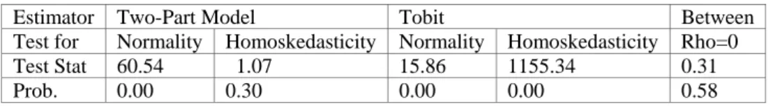
Table 1: Diagnostics To Choose Between Estimators
Estimator Two-Part Model Tobit Between
Test for Normality Homoskedasticity Normality Homoskedasticity Rho=0 Test Stat 60.54 1.07 15.86 1155.34 0.31
Prob. 0.00 0.30 0.00 0.00 0.58
In the Tobit case, the results lead to strong rejections of homoskedasticity and normality. For the two-part model, normality is rejected and homoskedasticity accepted. However, in the two-part model neither is a necessary condition for consistency (Cameron, A C and Trivedi 2009, p.541). The test on covariance between errors in different stages was calculated by running a Heckman model without an exclusion restriction, and independence (a key assumption of the Two-Part Model) cannot be rejected. These results point toward the Two-Part model as being the most appropriate.
Period Averaging
A further decision regarding the econometric approach is whether to use yearly data, or period averaged. Neumayer uses yearly data in his estimates and calculates clustered standard errors in the first step, and Huber/White/Sandwich estimator of variance in the second step. He reports that standard errors “are robust to towards arbitrary heteroskedasticity and serial correlation” (Neumayer 2003b, p.50.) It does not appear that these decisions regarding standard errors are in fact adequate to deal with serial correlation, as the Huber/White/Sandwich estimator is designed to deal with heteroskedasticity not serial correlation. The clustering of residuals is a complex topic, but does not by itself guard against bias from serial correlation. Tests for (first order) serial correlation using Neumayer’s (2003b) data and specification reject the null hypothesis of no serial correlation for every bilateral donor3 (see Drukker 2003 for information regarding this test). This is unlikely to be a problem confined to one paper, as much of the research is likely to suffer from this problem. The main strategy employed here to circumvent the problem of serial correlation is to use 5-year period averages. 5 year averages can be thought of as ‘snap shots’ of the average practice of that period. As annual data is not included, there is less opportunity for persistent independent variables to bias the estimated betas. This approach also diminishes the potential problem of high volatility in aid transfers, and divides the time period neatly into the three ‘eras’ used.
The Main Specification
It is worth noting throughout the discussion the trade off between data availability and specification accuracy. For example, when examining policy, many variables available do not exist for the first years of the data. It might also be desirable to use information on poverty rather than income, but sufficient data simply do not exist. Throughout the discussion there are similar trade-offs. A parsimonious specification is first chosen, with more information being used in robustness checks or to answer specific questions. This means the time period runs from 1982-2006, in five 5-year time periods. A full description of the data can be found in the appendix.
Dependent Variable
The choice of dependent variable is more contentious than might be expected. In the framework used here, a government allocates a proportion of its budget in time t to aid. The income of the country, the proportion of that which becomes the government budget and the resultant allocation to the aid agency is all thought exogenous. From this budget a donor first decides between multilateral agencies and bilateral recipients. It then allocates between different recipient countries, and is influenced by four factors: poverty, population, policy and proximity. The paper models only the last step, thus treating all previous steps as exogenous. The dependent variable is then the logged percentage share of a donor’s total aid budget commitments in a given year to a given recipient, that is
where the subscript i refers to the donor, and j to the recipient. In this state it is normally distributed, which is desirable for the estimator used. Commitments are used as they more accurately portray the wishes of the donor. Other papers have used aid per capita, aid as a share of GDP and nominal aid as the dependent variable. The first does not reflect the decision that the donors make as closely, as donors commit aid in nominal terms for a specific period of time. The second approach means that the dependent variable is a function of aid commitments but also a recipient’s income. This may overstate a poverty bias, as poorer countries will by definition receive ‘higher’ aid commitments. The third suggested variable is likely to be influenced by fluctuations in a donor’s budget. Time dummies would correct for this to some extent, but not completely.
Poverty
Monetary measures of poverty are the most common due to the lack of reliable alternatives. Poverty headcount data simply do not exist on the scale needed, and for this reason logged GDP per capita data is used in the parsimonious specification. This is likely to be the data that the donor had access to when making the decision.
Population
Logged Population is used to capture what is in essence another indicator of need – the population. By making population a factor in its own right, and separating it from poverty, a donor’s decision regarding China and India do not dominate the identification of poverty coefficients. While the population size in India and China presents a problem
for the applied researcher seeking to disentangle the effect of poverty and population upon aid receipts, this solution is more desirable than succumbing to the temptation to exclude them as special cases, which means ignoring the majority of the developing world. Furthermore, as we are modelling the impact of these factors in the mind of the donor, we can be reassured that this approach is similar to the approach found in donors’ performance based allocation formulas that are available to the public (where typically income and population are included separately, the latter discounted at the rate . ).
Policy
For the more parsimonious specification, many of the more sophisticated measures cannot be used due to data availability. We follow Neumayer (2003b) in using the Freedom
Index and PTS. The FreedomIndex is combined total of political rights and civil liberties,
transformed to a scale from 2 (worst) to 14 (best), and taken from Freedom House. The Political Terror Scale (PTS) runs from 1 (worst) to 5 (best) and describes the level of terror or absence of the rule of law. The information is ultimately taken from two sources: Amnesty International and the US State department. While the data may or may not capture accurately the policy outcomes or inputs of a recipient, they are likely to capture the level of policy as perceived by donors. Indeed, they have been used by some donors explicitly (e.g. the Millennium Challenge Account). The data also suffer considerably less from missing data than alternate measures over the period examined.
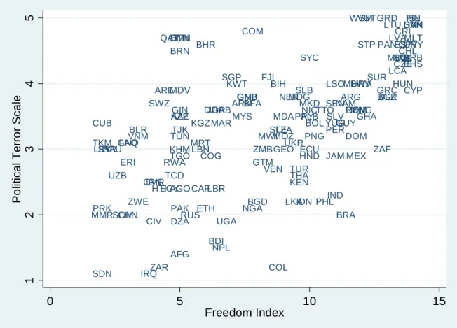
To give a better understanding of the policy data, a few brief examples are presented. There are no signs of multicollinearity between the two variables, but they are positively correlated with a correlation coefficient of 0.51. Both are negatively skewed, with mean scores of 3.4 and 8.6 for PTS and Freedom respectively. In 2006 for the PTS, the nine countries to score four or worse were Afghanistan, Central African Republic, Columbia, Congo (DRC), Iraq, Myanmar, Nepal, Sudan and Sri Lanka. In 2006, the nine worst scores for Freedom were held by Cuba, North Korea, Libya, Myanmar, Saudi Arabia, Sudan, Syria, Turkmenistan and Uzbekistan. While there is obviously some overlap, the distinction is clear in many cases. On a regional level, African countries in 2006 scored higher on the Freedom variable (by 1.5) than the rest of the sample, but had no real difference in PTS. Some countries show low levels of democracy but an absence of
political terror: Qatar, Swaziland and United Arab Emirates. Others show relatively high scores for democracy but low levels for PTS: Brazil, India and the Philippines. However, the overall pattern is of a positive relationship between the two variables, as can be seen in Figure 2.
Figure 2: PTA and Freedom Index, 2006 with ISO Labels
Note: ISO labels are used as markers. Those of interest include: SDN Sudan, COL Columbia, IRQ Iraq, BRA Brazil, CUB Cuba, BRN Brunei, BHR Bahrain and COM Comoros.
Proximity
Proximity can be understood in many ways. Religion, Language and Colony variables describe the cultural and historical links between two nations. The religion variable measures the percentage of the recipient’s population that adhere to the largest faith in the donor country. For example, for Japan it measures the percentage of recipient population that are Buddhist, and for USA Christian. Language is a dummy which takes the value 1 if at least nine percent of the donor and recipient populations speak the same language. This threshold is inherited from the data used (CEPII), but represents the most accurate
AFG ALB DZA AGO ARG ARM AZE BHS BHR BGD BRB BLR BLZ BEN BTN BOL BIH BWA BRA BRN BGR BFA BDI KHM CMR CAN CPV CAF TCD CHL CHN COL COM ZAR COG CRI CIV HRV CUB CYP CZE DNK DJI DOM ECU EGY SLV GNQ ERI EST ETH FJI FIN GAB GMB GEO GHA GRC GRD GTM GIN GNB GUY HTI HND HUN ISL IND IDN IRN IRQ JAM JOR KAZ KEN PRK KWT KGZ LAO LVA LBN LSO LBR LBY LTU MKD MDG MWI MYS MDV MLI MLT MRT MUS MEX MDA MNG MAR MOZ MMR NAM NPL NIC NER NGA OMN PAK PAN PNG PRY PER PHL POL QAT ROM RUS RWA WSM STP SAU SEN SYC SLE SGP SVK SVN SLB SOM ZAF LKA LCA SDN SUR SWZ SYR TJK TZA THA TGO TTO TUN TUR TKM UGA UKR ARE URY UZB VUT VEN VNM YUG ZMB ZWE 1 2 3 4 5 Po lit ica l T e rro r Sca le 0 5 10 15 Freedom Index
and complete dataset available on bilateral common languages. Colony is a similar dummy, but with colonial history. To capture trade interests, Exports is a variable which is the logged share of donor country exports that a recipient represents. This should capture the importance of the recipient to a donor’s export sector. To measure military importance Arms is a measure of the total amount of arms exports from the donor to the recipient in that year. This should capture any particularly strategic military relationships, USA-Egypt for example. Another measure to capture military proximity, only available for the USA, is the value of American bilateral military aid transfers (these are not included in ODA).
A Proximity Index is constructed for use in answering questions 2-4, where proximity is
included as a control rather than a variable of direct interest. While tests show multicollinearity is not a concern in later questions the size of the dataset is more restricted, and the index allows clearer interpretation by aggregating the cultural, religious, historical and military links. The proximity index was constructed by regressing Arms (as a dummy), US military Grants, Religion, Language and Colony and controls in a similar regression to that reported in Table 3. The relevant coefficients were then used as weights in the proximity index, which was scaled so that the ‘closest’ country received a score of 1, and the ‘furthest’ country received a score of 0. In this form, the coefficient in the level stage can be interpreted as the difference between the most and least proximate countries. For the second stage, standardised coefficients are used and so interpretation is also clear. Regressions show a negligible loss of information. This index means proximity in questions 2-4 is represented by only two variables: Trade and Proximity Index, and thus facilitates interpretation.
Which Donors?
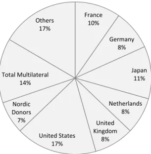
Figure 3: 2006 ODA Commitments by Donor, as a % of Total Commitments4
The literature tends to either analyse either average donor behaviour (with deviations from this) or a collection of individual donors. We employ the latter method5, focusing throughout on seven donors. The donors found in
Figure 3 are used, except that multilateral and ‘others’ are excluded, and Sweden is chosen to represent the Nordic Donors.
4
Results
Question 1: What are the Donor Differences?
In order to answer the above question, we estimate the parsimonious specification over the entire time period. Table 2 and 3 report the results for step 1 and 2 respectively, and Table 4 Wald statistics for the four factors.
4 Authors Calculations, based on OECD data, where all commitments are included.
5 This decision is motivated partly by a belief in the heterogeneity of donors which implies some difficulties in aggregating them for current research. Furthermore, ‘average donor behaviour’ can be a misleading term, as it is an unweighted average. Thus what is happening to donors on average could be quite different to what is happening to aid on average. This later concept will be dominated by the 7 donors chosen, who accounted for over 60% of aid commitments in 2006. France 10% Germany 8% Japan 11% Netherlands 8% United Kingdom 8% United States 17% Nordic Donors 7% Total Multilateral 14% Others 17%
Table 2: 1982-2006, Parsimonious Specification, Eligibility Stage
France Germany Japan Netherlands Sweden USA UK Ln(GDP) -0.44*** -0.36*** -0.42*** -0.46*** -0.30*** -0.64*** -0.47*** (5.17) (4.39) (6.09) (5.90) (4.02) (7.95) (5.85) Ln(Population) -0.14* -0.096 -0.20*** 0.14* 0.29*** -0.12* 0.0046 (2.06) (1.43) (3.64) (2.44) (5.06) (2.01) (0.080) Freedom Index 0.039 0.038 0.10*** 0.068** 0.12*** 0.11*** 0.077** (1.45) (1.49) (4.46) (2.84) (4.89) (4.07) (3.10) Political Terror Scale -0.28** -0.25* -0.34*** -0.32*** -0.10 -0.36*** -0.27** (2.63) (2.30) (3.33) (3.45) (1.22) (3.43) (2.77) Religion 0.0064** 0.0077*** -0.00058 0.0069*** 0.0030 0.0054* 0.0056** (2.99) (3.39) (0.12) (3.65) (1.77) (2.42) (2.74) Arms 0.0056* 0.0092* -0.0064 -0.033 0.00028 0.0037 (2.04) (2.36) (1.57) (1.50) (0.52) (1.76) Exports 0.085 -0.99* 0.68** -2.28*** -1.23* 0.25 -0.75 (0.16) (2.01) (2.67) (3.53) (2.52) (0.88) (1.30) Colony -0.40 -0.43 0.20 (1.67) (0.98) (0.94) Language 0.54* 0.24 0.38* 0.39 (2.04) (1.75) (2.24) (1.71) US Military Grants -0.013 (1.66) Pseudo R-squared 0.153 0.182 0.118 0.293 0.159 0.255 0.201 Observations 532 532 527 570 530 523 531 Non-Recipients 96 90 91 201 296 123 138
Correctly predicted aid recipients 83.60% 85.71% 83.23% 79.71% 66.06% 83.07% 80.74% Correctly predicted non-recipients 50.00% 54.29% 50.00% 73.29% 71.52% 70.27% 67.57%
Note: This was estimated using a Probit model, without clustered errors. Coefficients are not standardised. 3, 2 and 1 Star(s) denote the 1, 5 and 10 % significance levels respectively.
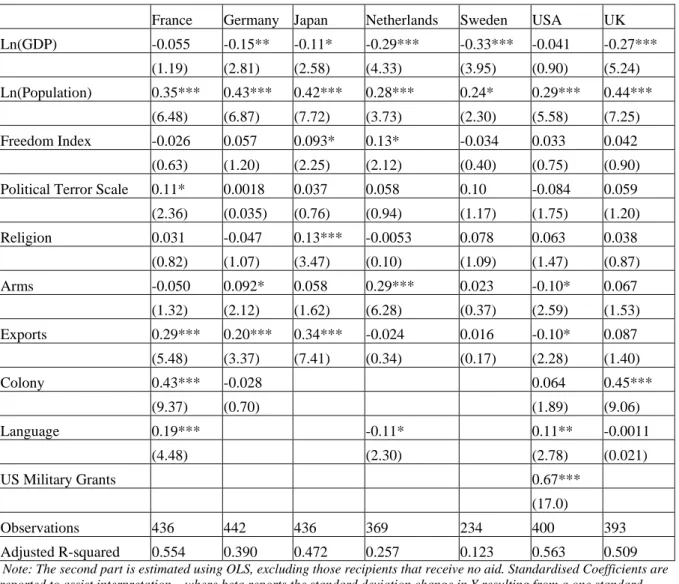
Table 3: 1982-2006, Parsimonious Specification, Level Stage (Standardised Coefficients)
France Germany Japan Netherlands Sweden USA UK
Ln(GDP) -0.055 -0.15** -0.11* -0.29*** -0.33*** -0.041 -0.27*** (1.19) (2.81) (2.58) (4.33) (3.95) (0.90) (5.24) Ln(Population) 0.35*** 0.43*** 0.42*** 0.28*** 0.24* 0.29*** 0.44*** (6.48) (6.87) (7.72) (3.73) (2.30) (5.58) (7.25) Freedom Index -0.026 0.057 0.093* 0.13* -0.034 0.033 0.042 (0.63) (1.20) (2.25) (2.12) (0.40) (0.75) (0.90) Political Terror Scale 0.11* 0.0018 0.037 0.058 0.10 -0.084 0.059
(2.36) (0.035) (0.76) (0.94) (1.17) (1.75) (1.20) Religion 0.031 -0.047 0.13*** -0.0053 0.078 0.063 0.038 (0.82) (1.07) (3.47) (0.10) (1.09) (1.47) (0.87) Arms -0.050 0.092* 0.058 0.29*** 0.023 -0.10* 0.067 (1.32) (2.12) (1.62) (6.28) (0.37) (2.59) (1.53) Exports 0.29*** 0.20*** 0.34*** -0.024 0.016 -0.10* 0.087 (5.48) (3.37) (7.41) (0.34) (0.17) (2.28) (1.40) Colony 0.43*** -0.028 0.064 0.45*** (9.37) (0.70) (1.89) (9.06) Language 0.19*** -0.11* 0.11** -0.0011 (4.48) (2.30) (2.78) (0.021) US Military Grants 0.67*** (17.0) Observations 436 442 436 369 234 400 393 Adjusted R-squared 0.554 0.390 0.472 0.257 0.123 0.563 0.509
Note: The second part is estimated using OLS, excluding those recipients that receive no aid. Standardised Coefficients are reported to assist interpretation – where beta reports the standard deviation change in Y resulting from a one standard deviation change in X Non-standardised coefficients can be found in the Appendix, Table A8. Following standard practice, this does not apply to the dummy variables (colony, language, religion) which are instead the standard deviation change in Y resulting from a one unit change in X. 3, 2 and 1 Star(s) denote 1, 5 and 10 % significance levels respectively.
Table 4: Wald Tests
France Germany Japan Netherlands Sweden USA UK
1 st Step Poverty 6.950*** 4.091** 11.55*** 17.46*** 9.454*** 15.95*** 11.30*** Population 1.268 0.579 5.810** 2.678 16.41*** 1.645 0.00251 Policy 4.357 3.037 13.05*** 8.406** 15.08*** 11.90*** 7.582** Proximity 6.11 6.669 3.506 27.06*** 9.973** 11.84** 9.564* 2 nd Step Poverty 0.116 4.812** 2.374 18.52*** 7.734*** 0.827 14.16*** Population 23.17*** 26.14*** 34.60*** 2.011 2.279 24.05*** 31.78*** Policy 1.202 0.142 3.698 1.647 3.198 2.461 2.441 Proximity 87.03*** 8.492* 33.70*** 19.14*** 2.53 323.6*** 63.82***
Note: The Wald Test statistics is shown, with stars denoting the 1, 5 and 10 % significance levels. The Wald statistic has a largesample Chisquared distribution.
Here, we can compare aid allocation between donors, having in essence estimated a donor’s average allocation behaviour over a 25 year period. The Wald statistics allow us to attribute explanatory power to the competing factors of the 4P framework. Using these statistics, we find that all donors use income as a determinant of aid eligibility (less so for Germany and France), but the same is not true at the levels stage. Amongst the donors reported, we can identify three groups of poverty sensitivity: High (Netherlands, Sweden and the UK), medium (Germany and Japan) and low (USA and France). Looking at population, this is only a significant determinant at the eligibility stage for two donors. For Japan this appears to be in excluding larger countries (most probably a China effect), and for Sweden excluding smaller countries. Sweden selects fewer recipients than other donors, and so this is unsurprising. All donors have positive coefficients for population at the levels stage, and exhibit evidence of a small-country bias.
Four of the seven donors have significant Wald statistics at the eligibility stage for Policy, and none of the seven at the levels stage. Inspection of the coefficients shows that every donor has a positive relationship with the Freedom coefficient and a negative one for Political Terror Scores. Interestingly, for all donors the average PTS score for recipients of aid is higher than for non-recipients. This means that on average donors are more likely to give aid to countries with better human rights, but this result reverses when controlling for other factors. Tests show multicollinearity is not problematic. It may be that donors are less interested in human rights than other factors, and it is simply correlated with poverty or proximity. In the second stage France, Japan and the Netherlands exhibit some signs of Policy sensitivity, but not when tested overall. This implies policy sensitivity has not been a major feature of any donor’s allocation principles when averaged over the last 25 years. This is particularly apparent when comparing the size of the Wald statistics with other factors.
Wald statistics show that the Proximity Variables are significant for every donor at some stage, but show large differences between donor in the level of significance and the constituent parts that underlie this significance. Germany and Sweden only have significant Wald statistics at one step, and a relatively low score in the other. For Sweden this manifests itself in a (weakly significant) negative coefficient on trade in the levels
stage and for Germany it is a positive coefficient on the trade variable at the 2nd Step. The Netherlands has a negative coefficient for trade but a positive coefficient for Religion at the first stage. At the levels stage it gives more to countries that purchase its arms and less to recipients with which it shares a language. For the Netherlands, many countries share a language as its own population are often multilingual, i.e. the dummy includes French, German and English speaking countries. The UK and France have much higher Wald statistics for proximity than those donors already discussed. For France almost all proximity coefficients at both stages are positive. The standardised coefficients show the biggest effect is for former colonies at the levels stage, but language and exports are also positive. For the UK, the biggest effect at the levels stage is of former colonies. For both France and the UK being a former colony results in 40% of a standard deviation increase in aid: roughly 0.7% of the aid budget for both donors.
The USA has an almost incomparably high Wald statistic for proximity. At the eligibility stage they are not too dissimilar from other donors. However, at the level stage they have positive and relatively large coefficients for US military grants and language. For the USA the colony dummy is identifying solely on the Philippines, and is thus effectively a dummy for the Philippines (which was a colony of the USA for almost half a century). The coding of the language variable (at least 9% of the recipient-donor pair speaking the same language) means this includes Hispanic America, and is thus positive at both stages. The military variable has the largest coefficient across the standardised coefficients, which suggests American aid is often used to reward or reinforce military relationships. It is likely that this relationship trumps any relationship through arms sales, and thus this later coefficient is found negative.
The USA is different from other donors in their relationship to trade. Most donors show a positive and significant relationship, whereas for the USA it is negative and significant. It was on the basis of this coefficient that Berthélemy (2006) classified some donors as selfish and others as altruistic. However, the literature makes clear that there are several channels though which aid could be used to promote exports (Osei, Morrissey, and Lloyd 2004), and it is difficult to rule out aid being used to promote exports on the basis of a negative coefficient. For example, aid could be given to recipients that currently import a
small amount of goods from the donor country, with the aim of increasing this over time (Lloyd, McGillivray, Morrissey, and Osei 2000). The results show that American and British aid does not have a positive relationship with trade flows, in contrast to other donors.
Question 2: what are changes over time?
To answer the previous question, we looked at each donor in turn over the 25 years. To answer how allocation practice has evolved over time, we look specifically at three periods: Cold War, post Cold War and post 9/11. The post 2001 time period has been studied for American aid, but not for others. It is possible that other donors were affected in the same way, but it also offers some evidence regarding policy selectivity. Separate results by donor, time period and stage are provided in the Appendix (Table A 1- Table A 7). To give some initial measure of the extent to which allocation practice has changed over the period, Chow tests were conducted on the sample. These are calculated by augmenting the previous regression with all variables of the variables interacted with dummies for the CW period, and the period after the September the 11th terrorist attacks. The Chow test is essentially a test of whether there has been a significant change in the underlying relationships, as these new variables contain no new information. If there was a consistent relationship between the dependent and independent variables the coefficients on these new variables would be equal to zero. The below statistics are in essence tests of that assumption.
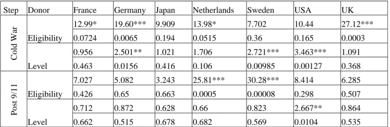
Table 5: Chow Tests for Changed Relationships
Step Donor France Germany Japan Netherlands Sweden USA UK
Co ld War Eligibility 12.99* 19.60*** 9.909 13.98* 7.702 10.44 27.12*** 0.0724 0.0065 0.194 0.0515 0.36 0.165 0.0003 Level 0.956 2.501** 1.021 1.706 2.721*** 3.463*** 1.091 0.463 0.0156 0.416 0.106 0.00985 0.00127 0.368 Po st 9 /11 Eligibility 7.027 5.082 3.243 25.81*** 30.28*** 8.414 6.285 0.426 0.65 0.663 0.0005 0.00008 0.298 0.507 Level 0.712 0.872 0.628 0.66 0.823 2.667** 0.864 0.662 0.515 0.678 0.682 0.569 0.0104 0.535
Note: Chow statistics have an F distribution and are reported above with the P value below. Results refer to the parsimonious specification. The statistics are relative to the period 1992-2001.
Table 5 shows joint significance tests by step, donor and period. Japan is the only donor that does not show significant differences in overall allocation policy over the twenty-five year period. The USA, Sweden and Netherlands are the only donors for whom the GWOT period is significantly different (and the USA is the sole donor for which it is significant at the level stage). The Cold War period, by contrast, sees changes for every donor apart from Japan. We can further break these differences down into differences using the 4P framework, for those donors that demonstrate significant differences.
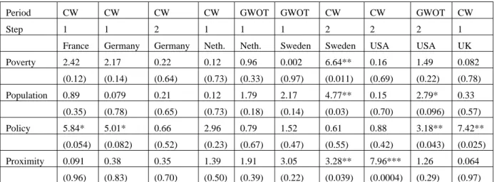
Table 6: Wald Statistics for Donors with Significant Changes, Using 4P Framework
Period CW CW CW CW GWOT GWOT CW CW GWOT CW
Step 1 1 2 1 1 1 2 2 2 1
France Germany Germany Neth. Neth. Sweden Sweden USA USA UK
Poverty 2.42 2.17 0.22 0.12 0.96 0.002 6.64** 0.16 1.49 0.082 (0.12) (0.14) (0.64) (0.73) (0.33) (0.97) (0.011) (0.69) (0.22) (0.78) Population 0.89 0.079 0.21 0.12 1.79 2.17 4.77** 0.15 2.79* 0.33 (0.35) (0.78) (0.65) (0.73) (0.18) (0.14) (0.03) (0.70) (0.096) (0.57) Policy 5.84* 5.01* 0.66 2.96 0.79 1.52 0.61 0.88 3.18** 7.42** (0.054) (0.082) (0.52) (0.23) (0.67) (0.47) (0.55) (0.42) (0.043) (0.025) Proximity 0.091 0.38 0.35 1.39 1.91 3.05 3.28** 7.96*** 1.26 0.064 (0.96) (0.83) (0.70) (0.50) (0.39) (0.22) (0.039) (0.0004) (0.29) (0.97)
Note: The Wald Test statistics is shown, with stars denoting the 1, 5 and 10 % significance levels. The Wald statistic has a large-sample Chi-squared distribution. CW denotes the cold war period 1982-1991, GWOT 2002-2006 and Neth., The Netherlands.
Using the breakdown in Table 6, and further inspection of individual coefficients, we can find the cause of the differences between periods. For France, the change is driven by an increasingly negative coefficient on PTS, perhaps as long-term recipients have received worse scores but aid has not decreased. The same can be said for Germany, although that is combined with an increasingly positive coefficient for Freedom. For Germany, the difference of the levels stage for the Cold War period does not have a single factor, but instead a multitude of small changes including decreasing poverty sensitivity. Both steps for the Netherlands and Sweden’s 1st Step can also be said to be a number of small changes. This is perhaps expected as they are smaller donors that focus more than other donors, and small adjustments in selecting aid recipients may still be identified. Sweden during the Cold War appears different in almost every factor in the levels stage. The coefficient on poverty actually decreased with the end of the cold war, whereas policy selectivity appears to have increased (but is still not significant). The coefficient during
the Cold War (for Sweden at the levels stage) on exports was positive, but this has become negative in the latter periods. For the USA, a number of changes occurred, including a decreasing importance of Freedom over time, and a more negative coefficient for PTS. The Proximity index was most positive and significant in the period 1992-2001. This is driven by a significant and positive effect of trade in the first step and significant and negative effect in the second. In the Cold War and GWOT periods the coefficient is insignificant at both levels. The UK has had an increasingly negative coefficient for PTS.
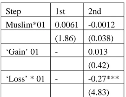
Moss et al. (2005) found three variables were successful in controlling for the effect of the GWOT on US aid allocation. The first was a dummy for four countries that received large aid increases since 2001: Iraq, Afghanistan, Jordan and the Palestinian Territories. The second was a dummy for recipients that saw large drops (which, it is argued, partially financed the aforementioned increases) in aid: Israel, Egypt and Bosnia Herzegovina. The third (which was less successful) was an interaction term for the percentage of Muslim population and a dummy for years after 2001. Retesting these variables for the second stage of US allocation (Table 7) finds only the dummy for those countries that receive less aid is significant, but that this variable is highly significant and represents 30% of a standard deviation fall in aid receipts as well as increased likelihood of censoring.
Table 7: Retesting the GWOT dummies
Step 1st 2nd Muslim*01 0.0061 -0.0012 (1.86) (0.038) ‘Gain’ 01 - 0.013 (0.42) ‘Loss’ * 01 - -0.27*** (4.83)
Note: Standardised Coefficients are reported to assist interpretation – where beta reports the standard deviation change in Y resulting from a one standard deviation change in X. Other variables included, but not reported: these variables are augmenting the parsimonious specification.
Question 3: has poverty selectivity increased?
Augmenting the parsimonious regression equation with income interacted with a period dummy allows us to estimate poverty selectivity by period, while still controlling for the other factors (the normal income variable is, of course, excluded). Table 8 reports only the poverty coefficients but they were obtained in a regression using the parsimonious specification over the 25-year time period.
Table 8: Income Coefficients: by Step, Period, Stage and Donor
France Germany Japan Netherlands Sweden USA UK
1st st age 1982- -0.26*** -0.17* -0.38*** -0.37*** -0.35*** -0.63*** -0.35*** 1986 (3.40) (2.25) (5.15) (5.01) (4.71) (8.44) (4.54) 1987- -0.29*** -0.19** -0.37*** -0.43*** -0.37*** -0.63*** -0.36*** 1991 (3.92) (2.58) (5.08) (5.85) (4.94) (8.52) (4.76) 1992- -0.32*** -0.23** -0.41*** -0.44*** -0.51*** -0.64*** -0.42*** 1996 (4.29) (3.18) (5.64) (5.98) (6.54) (8.80) (5.55) 1997- -0.32*** -0.24*** -0.42*** -0.45*** -0.30*** -0.62*** -0.43*** 2001 (4.41) (3.45) (5.92) (6.21) (4.15) (8.65) (5.85) 2002- -0.32*** -0.24*** -0.42*** -0.52*** -0.30*** -0.60*** -0.44*** 2006 (4.49) (3.49) (5.98) (7.11) (4.13) (8.66) (6.00) 2n d St age 1982- -0.29* -0.36** -0.33** -0.76*** -1.00*** -0.27* -0.86*** 1986 (2.39) (2.74) (2.61) (3.97) (4.53) (2.35) (6.02) 1987- -0.30* -0.42** -0.32* -0.82*** -1.09*** -0.37** -0.90*** 1991 (2.47) (3.12) (2.42) (4.35) (4.73) (2.94) (6.01) 1992- -0.31* -0.48*** -0.33* -0.83*** -0.57*** -0.46*** -0.87*** 1996 (2.51) (3.43) (2.53) (4.15) (3.67) (3.55) (5.85) 1997- -0.30* -0.56*** -0.41** -0.91*** -1.44*** -0.41** -0.93*** 2001 (2.39) (4.03) (3.11) (4.59) (5.11) (3.08) (6.33) 2002- -0.33** -0.59*** -0.43** -0.92*** -1.54*** -0.39** -0.93*** 2006 (2.66) (4.25) (3.28) (5.34) (5.40) (2.90) (6.41)
Note: 2nd Stage standardised coefficients are reported, with T statistics in parentheses.
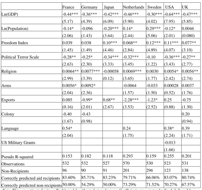
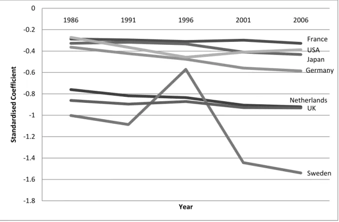
The first stage shows evidence of a small increase in the coefficient for some donors. As there is only a single variable representing poverty, the coefficients from stage 2 of the regression can be easily plotted, see Figure 4. This easily allows us to compare donors, and any changes over time relative to differences between donors. France, the USA, Japan and Germany all have coefficients of between -0.2 and -0.6 over the 25 year period. Of these, only the USA has become less poverty-sensitive in recent years – this is possibly an effect of the GWOT. While France has remained fairly static over the period,
Japan and Germany have become more poverty focused. The Netherlands and the UK both started significantly more poverty-sensitive, and have increased this over the period. For both donors, a 1 standard deviation difference in income per capita implies a response in aid budget share of almost one standard deviation. Sweden is even more poverty focused at this second step, but less so at the first step. The big decrease in poverty sensitivity in the 1992-1996 period is reflected by a larger coefficient for poverty in the first stage. We can divide the donors into two: the poverty sensitive donors (Netherlands, UK and Sweden) and the less poverty sensitive donors (France, Germany, Japan and USA). While there is some downward movement of the 25-year period, the largest differences are clearly between different donors, rather than between time periods.
Figure 4: Poverty Sensitivity Coefficients 1982-2006 Level Stage, by Donor
Question 4: has policy selectivity increased?
In order to examine the question of more recent changes to policy selectivity, we can augment the parsimonious specification. This means taking advantage of some of the more sophisticated variables available, at the cost of losing some years of data6. The motivation for suspecting that policy selectivity has increased is the work of Burnside and Dollar (2000) and
6We lose two time periods: 19821986 and 19871991. The data is available from the year 1996, and this one observation is used for the 19921996 period.
France Germany Japan Netherlands Sweden USA UK ‐1.8 ‐1.6 ‐1.4 ‐1.2 ‐1 ‐0.8 ‐0.6 ‐0.4 ‐0.2 0 1986 1991 1996 2001 2006 Standardised Coefficient Year
the apparent move from conditionality toward selectivity. The variable chosen is the
corruption variable taken from the Worldwide Governance Indicators (WGI) dataset. This is produced by the World Bank and uses a number of inputs to measure corruption on a scale between -2.5 (most corrupt) and 2.5 (least corrupt, although where standardised coefficients are reported this scale is somewhat immaterial). This variable has previously been used, but never as extensively (Hout, W. 2007b used all of the WGI variables with time variation, but only for three donors;Neumayer 2003b used one observation over the whole time period). Corruption is chosen as it is the most easily measured and widely discussed aspect of policy selectivity, and does not introduce problems of multicollinearity. When corruption is included in the specification as the sole representative of policy (results not reported), it is virtually always insignificant for each donor and step. The only exception is for the 2nd step coefficient for the USA, where it is found to be negative (i.e. more corrupt countries receive more aid). It is possible however that any policy changes are most evident in recent years. For this reason,
Table 10 show the coefficients for policy variables at the first and second stages, when corruption is interacted with a dummy for different periods. If there was Policy Selectivity, we would expect to find positive and significant coefficients.
Table 9: 1992-2006 Main Specification Eligibility Stage, Augmented With Policy Variables Interacted With Time Dummies
France Germany Japan Netherlands Sweden USA UK
Ln(GDP) -0.41*** -0.36*** -0.39*** -0.48*** -0.35*** -0.54*** -0.52*** (4.00) (3.58) (3.83) (4.69) (3.67) (5.41) (4.87) Ln(Population) -0.093 0.066 -0.12 0.25*** 0.28*** -0.13 0.10 (1.32) (0.91) (1.61) (3.76) (3.98) (1.95) (1.48) Freedom Index 0.093*** 0.12*** 0.14*** 0.11*** 0.13*** 0.17*** 0.15*** (3.53) (4.45) (4.49) (3.62) (4.36) (5.91) (5.32) Political Terror Scale -0.51*** -0.53*** -0.40** -0.55*** -0.27* -0.53*** -0.57***
(3.70) (3.75) (2.72) (4.37) (2.44) (3.80) (4.26) Control of Corruption 0.076 0.13 0.028 0.020 0.68*** 0.057 0.19 (0.33) (0.57) (0.12) (0.096) (3.30) (0.25) (0.80) Corruption * 2001 0.74 1.55 -0.25 1.88 -4.47*** -0.92 0.46 (0.58) (1.19) (0.19) (1.55) (3.81) (0.73) (0.36) Corruption * 2006 -0.59 -0.36 -1.89 2.76* -5.25*** -2.54 -0.31 (0.45) (0.26) (1.33) (2.32) (4.37) (1.96) (0.23) Exports -0.37 -1.58** 0.49 -3.46*** -1.65** 0.92* -1.37 (0.57) (3.01) (1.51) (4.00) (2.77) (2.10) (1.85) Proximity Index 0.049 -0.0093 2.46 -0.24 -0.20 -2.07 0.65** (0.17) (0.016) (0.19) (1.34) (0.64) (1.95) (2.77) Observations 379 379 317 398 378 376 379 Pseudo R-squared 0.162 0.211 0.169 0.318 0.237 0.247 0.266
Table 10: 1992-2006 Main Specification Level Stage,
Augmented With Policy Variables Interacted With Time Dummies
France Germany Japan Netherlands Sweden USA UK
Ln(GDP) -0.11* -0.18** -0.10 -0.27*** -0.34*** -0.075 -0.30*** (2.00) (2.94) (1.65) (3.45) (3.61) (1.60) (5.04) Ln(Population) 0.24*** 0.41*** 0.43*** 0.38*** 0.37** 0.26*** 0.53*** (3.78) (5.63) (5.92) (4.07) (3.23) (4.96) (7.11) Freedom Index 0.034 0.057 0.098 0.29*** 0.12 0.089 0.14* (0.67) (0.99) (1.61) (3.60) (1.23) (1.84) (2.33) Political Terror Scale 0.034 -0.041 -0.012 -0.077 -0.018 -0.052 0.059
(0.58) (0.61) (0.16) (0.86) (0.17) (0.96) (0.93) Control of Corruption -0.014 0.027 -0.054 -0.14 -0.18 -0.089 -0.12 (0.19) (0.33) (0.65) (1.41) (1.05) (1.41) (1.59) Corruption * 2001 0.012 0.075 0.071 0.14 0.20 -0.057 0.061 (0.23) (1.22) (1.11) (1.86) (1.54) (1.18) (1.08) Corruption * 2006 -0.0052 0.025 0.027 0.24** 0.29* -0.070 0.040 (0.10) (0.42) (0.44) (3.32) (2.19) (1.49) (0.74) Exports 0.34*** 0.29*** 0.34*** -0.14 -0.17 -0.14** 0.072 (5.58) (4.44) (5.46) (1.52) (1.56) (3.00) (1.06) Proximity Index 0.54*** -0.051 0.051 0.073 0.12 0.73*** 0.44*** (12.2) (1.08) (1.03) (1.14) (1.58) (18.6) (9.33) Observations 297 294 253 228 174 283 257 Adjusted R-squared 0.555 0.397 0.436 0.201 0.178 0.644 0.525
Note: Standardised Coefficients are reported to assist interpretation – where beta reports the standard deviation change in Y resulting from a one standard deviation change in X. Other variables not reported, these variables are augmenting the parsimonious specification.
Table 9 shows the results for the first step. Only Sweden has a positive coefficient for corruption but this is only for the period 1992-1996, and in later years it is significant and negative. The Netherlands show evidence of an increased coefficient on corruption, but for most donors there is little change. At the levels stage (
Table 10) the Freedom and PTS coefficients are typically insignificant, the exceptions being positive coefficients for the UK and Netherlands. There is scant evidence of an increasing importance of corruption; the Netherlands and Sweden being exceptions to this. In the case of the Netherlands, this is particularly interesting as it is then sensitive to corruption at both steps. There is (insignificant) evidence of a negative relationship between US aid and high levels of corruption, and of this increasing over the period. It should be remembered that the augmented coefficient should be interpreted in conjunction with the standard coefficient, e.g. the coefficient corruption for the Netherlands in 2006 is 0.14 0.24 0.10, so a one standard deviation increase in the control of corruption results in 10% of a standard deviation increase in aid budget share. Also, it is the change from previous practice that is found significant (or, in most cases, insignificant) rather than the practice itself. Overall, the picture is not one of high policy selectivity at either stage for most donors, but rather insignificant coefficients for policy variables.
The results are robust to exclusions of other policy variables, and the use of Corruption Perception Index data instead of the WGI data (not reported). We report one robustness test here; using the Country Policy and Institutional Assessment (CPIA) which is a dataset constructed by World Bank staff to measure economic and social policies. While criticised in some of the academic literature for being too closely related to growth (Dalgaard, Hansen, and Tarp 2004), some multilateral donors use it as a measure of policy. As it was not publicly available before 2005, a cross section averaged over the 2001-2006 period is reported here.
Table 11: Augmented with CPIA: 2001-2006 Cross Section, Eligibility Stage
France Germany Japan Netherlands Sweden USA UK
Ln(GDP) -0.064 -0.15 -0.37 0.45 0.027 -0.30 0.049 (0.15) (0.35) (0.68) (0.84) (0.052) (0.70) (0.10) Ln(Population) 0.20 0.70 0.39 1.35* 1.00* 0.45 0.81* (0.69) (1.80) (0.90) (2.32) (2.51) (1.64) (1.99) Freedom Index 0.15 0.27* 0.20 0.53* 0.098 0.16 0.54** (1.37) (2.07) (1.10) (2.47) (0.91) (1.42) (2.76) Political Terror Scale -0.70 -0.37 -0.35 -4.26** -1.22 0.040 -1.21 (1.25) (0.67) (0.52) (2.86) (1.82) (0.076) (1.84) Control of Corruption 0.91 0.83 0.35 5.54** 1.75 0.44 0.96
(1.01) (0.96) (0.26) (2.85) (1.83) (0.56) (0.91) CPIA -0.36 -0.35 -0.081 -1.12 0.017 -0.39 -1.15 (0.40) (0.39) (0.068) (0.94) (0.017) (0.48) (1.14) Exports -1.13 -15.2* -5.15 -19.1 -11.5* -2.59 -9.57 (0.12) (1.99) (1.28) (1.91) (2.34) (0.52) (1.85) Proximity Index -0.14 -1.19 -3.98 1.83* 1.54 10.3 1.03 (0.18) (0.92) (0.10) (2.02) (1.20) (0.62) (1.11) Observations 65 65 47 62 65 65 65 Pseudo R-squared 0.146 0.323 0.251 0.584 0.505 0.187 0.513
Table 12: Augmented with CPIA: 2001-2006 Cross Section, Levels Stage
France Germany Japan Netherlands Sweden USA UK
Ln(GDP) -0.14 0.12 0.21* -0.21 -0.21 0.051 -0.061 (1.03) (0.86) (2.06) (1.40) (1.27) (0.43) (0.54) Ln(Population) -0.35 0.42 0.72*** 0.90** 0.35 0.17 0.31 (1.43) (1.59) (4.11) (3.45) (1.17) (0.86) (1.41) Freedom Index -0.018 0.16 0.27 0.13 -0.089 0.081 0.041 (0.13) (1.00) (1.75) (0.65) (0.46) (0.61) (0.26) Political Terror Scale -0.15 -0.018 -0.019 0.44 0.10 -0.16 -0.13
(0.81) (0.095) (0.12) (1.76) (0.46) (0.93) (0.81) Control of Corruption -0.33 -0.12 0.059 -0.071 -0.29 -0.33* -0.16 (1.98) (0.66) (0.40) (0.32) (1.30) (2.24) (1.03) CPIA 0.31 -0.020 -0.33 0.069 0.53* 0.22 0.082 (1.82) (0.11) (1.96) (0.29) (2.26) (1.47) (0.51) Exports 0.66*** 0.27 0.20 -0.60** -0.25 -0.15 0.27 (4.31) (1.68) (1.62) (3.12) (1.09) (1.25) (1.90) Proximity Index 0.32* -0.090 0.076 -0.047 0.076 0.51*** 0.37*** (2.60) (0.77) (0.77) (0.32) (0.49) (4.58) (3.65) Observations 58 56 43 38 47 57 53 Adjusted R-squared 0.425 0.325 0.616 0.352 0.133 0.526 0.581
Note: Standardised Coefficients are reported to assist interpretation – where beta reports the standard deviation change in Y resulting from a one standard deviation change in X. Other variables not reported, these variables are augmenting the parsimonious specification.
Table 11 shows the policy variables for the first stage of the regression. The CPIA variable is not significant for any donor. It does however mean that the Freedom Index coefficient become positive, this is most likely due to the sample size restrictions of including the CPIA.