A
UTOMATED
S
EGMENTATION
OF THE
P
ERICARDIUM
U
SING
A
F
EATURE
B
ASED
M
ULTI
-
ATLAS
A
PPROACH
A
LEXANDER
N
ORL
EN
´
Master’s thesis
2014:E53
Faculty of Engineering
Centre for Mathematical Sciences
Mathematics
CE
N
T
RU
M
S
CI
E
N
T
IA
RU
M
M
A
T
H
E
M
A
T
ICA
RU
M
Abstract
Multi-atlas segmentation is a widely used method that has proved to work well for the problem of segmenting organs in medical images. But standard methods are time consuming and the amount of data quickly grows to a point making use of these methods intractable. In this work we present a fully automatic method for segmentation of the pericardium in 3D CTA-images. We use a multi-atlas ap-proach based on feature based registration (SURF) and use RANSAC to handle the large amount of outliers. The multi-atlas votes are fused by incorporating them into an MRF together with the intensity information of the target image and the optimal segmentation is found efficiently using graph cuts. We evaluate our method on a set of 10 CTA-volumes with manual expert delineation of the pericardium and we show that our method provides comparable results to a standard multi-atlas algorithm but at a large gain in computational efficiency.
Keywords: computer vision, medical image analysis, multi-atlas segmentation, feature based registration, Markov Random Fields, pericardium segmentation.
Acknowledgments
I would like to thank my supervisors Prof. Fredrik Kahl and Ass. Prof. Olof Enqvist for their valuable comments and insights regarding this project and the report. I would also like to take the opportunity to thank those who might be relatively tired of hearing me rambling about hearts and registration, but still for some reason find the energy to stay and listen.
Contents
1 Introduction 1
1.1 Problem Formulation . . . 2
1.2 Data Set . . . 3
1.3 Proposed Solution . . . 3
1.4 Contributions and Related Work . . . 5
1.5 Structure of the Report . . . 5
2 Theory 6 2.1 Image Registration . . . 6
2.2 Markov Random Fields . . . 8
2.3 Graph Cuts . . . 10
3 Method: Multi-atlas Segmentation 13 3.1 Feature Based Registration . . . 14
3.2 Intensity Based Registration . . . 18
4 Method: MRF Segmentation 21 4.1 MRF Formulation . . . 21
4.2 Maxflow . . . 25
4.3 Training . . . 25
5 Implementation and Evaluation Details 27 5.1 Registration . . . 27
5.2 Multi-atlas Segmentation . . . 29
5.3 MRF Segmentation . . . 29
6 Results 31 6.1 Registration and Multi-atlas Segmentation . . . 31
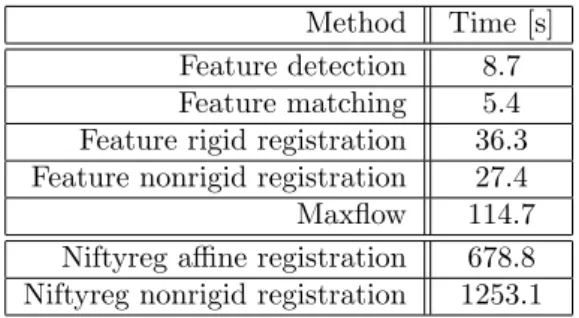
6.2 MRF Segmentation . . . 31 6.3 Runtimes . . . 32 6.4 Fat Estimation . . . 33 7 Discussion 34 7.1 Registrations . . . 34 7.2 MRF . . . 35 7.3 Computational Efficiency . . . 35
7.4 Comparison to Related Work . . . 35
7.5 Review of Algorithm . . . 36
List of Figures
1.1 a) A slice of a CT-volume of the heart. b) The same slice as in a) but with a manual delineation done by an expert of the pericardium (green) and the epicardial fat highlighted (red). . . . 1 1.2 A sagittal slice of one of the atlases. By aligning the labels of
sev-eral atlases (by estimating a transformation through registration) onto the target image we get a good estimate of the segmenta-tion. Each red line in this figure represents the boundary of an aligned labeling using feature based non-linear registration. The green line corresponds to the boundary of the gold standard (the manual labeling). . . 4 2.1 The grey nodes represent a 3⇥3 image. the nodes are connected
to its neighbors and all pixels are connected both to the source node s and the sink node t. All edges have costs we. The cut parts the graph so that no path exists between sand t and the pixels are separated into two sets: the pixels that are connected to sand the pixels that are connected to t. The minimal cut is the cut that separatest andsand has the minimal cost. Figure is found in [3]. . . 11 2.2 The grey nodes represent a small two node graph. Both nodes
are connected to each other and the source (denoted as 0) and the sink (denoted as 1). All edges have defined weightswe. . . . 12 3.1 a) One slice of an CT-volume. b) Corresponding slice of the
manual labeling. Together a) and b) form an atlas. . . 13 3.2 From left to right: the discretized second order partial derivative
in y- (Lyy) and xy-direction (Lxy), respectively. And the box approximation of these filters. . . 16 3.3 To evaluate the sum of all pixels⌃inside a box you only need to
evaluate and sum four elements in the integral imageI⌃ . . . 16 3.4 Haar wavelet filters in the x- and y directions. Dark areas has
weight 1 and white has weight +1. . . 17 5.1 A slice of a vote map constructed from 9 rigid feature based atlas
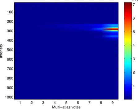
registrations. The vote map was blurred with a Guassian kernel to extract a target mask (the boundary of which are shown in red). 28 5.2 A typical histogram showing number of voxels in the training set
with number of multi-atlas votes on the x-axis and intensity bins on the y-axis. . . 30
7.1 An example of a part of a good segmentation. The red boundary is the boundary of the gold standard. The green line represents the boundary of the segmentation estimated by the feature based multi-atlas segmentation. The blue line corresponds to the same feature based multi-atlas segmentation incorporated into the MRF. 36 7.2 Here the MRF corrects the segmentation that is wrongly
esti-mated to being in the lung cavity. Red is gold standard, green multi atlas segmentation and blue is the segmentation also using the MRF. . . 37 7.3 In this example where the pericardium is visible (the intensities
are slightly brighter under the red line representing the boundary of the gold standard) we can clearly see the e↵ect of the intensity dependent boundary cost of the MRF. . . 37 7.4 If the multi-atlas segmentation is not satisfactory and the
peri-cardium is not clearly visible the segmentation will not represent the boundary accurately. . . 38 7.5 This figure shows a slice of the image on which our algorithm
performed poorest. In a way it summarizes the advantages and drawbacks of our algorithm. The segmentation fails in the top of this slice due to the image stretching further above the peri-cardium relative to the other atlases. This has a large e↵ect on the Jaccard index but arguably not as profound on the fat mea-surements. To the right and to the bottom left the pulmonary veins and the inferior vena cava pass through the pericardium and we can see that our algorithm struggle to close these areas in a way consistent with the the experts delineation. On the bottom left the multi-atlas segmentation was not so accurate. The e↵ect of the MRF is clear where it successfully corrects the segmenta-tion that passes through the lung and half of the fatty area to the left but not on the bottom left where the multi-atlas registrations were too far from the correct boundary. . . 39
Chapter 1
Introduction
According to the World Health Organization cardiovascular diseases are the number one cause of death worldwide [24]. Visceral adipose tissue, which is fat surrounding internal organs, may be a marker for greater risk of di↵erent metabolic and cardiovascular diseases. Epicardial fat is the visceral fat depot enclosed by the pericardial sac. In other words it is the fat located around the heart but inside of pericardial sac that surrounds the heart. In Figure 1.1 we see a 2D slice of a CT volume with the pericardium and the epicardial fat highlighted. In recent years, several studies have shown a relationship be-tween increased volume of epicardial fat and coronary artery disease, coronary plaque, adverse cardiovascular events, myocardial ischemia and atrial fibrilla-tion. Because of this scientific evidence there is a need for further investigation concerning the prognostic importance of epicardial fat, see [6].
Figure 1.1: a) A slice of a CT-volume of the heart. b) The same slice as in a) but with a manual delineation done by an expert of the pericardium (green) and the epicardial fat highlighted (red).
The Swedish CArdioPulmonary bioImage Study (SCAPIS) is a unique re-search project that started in 2012 in a collaboration between Sahlgrenska Uni-versity Hospital, the UniUni-versity of Gothenburg and the Swedish Heart-Lung
1.1. PROBLEM FORMULATION
Foundation. It is a large scale studie which aims at collecting CT, MR and ul-trasound images form 30 000 men and women between the ages of 50-65 years. This database, which will be the largest of its kind, will then serve as a national knowledge base for the study of identifying risk factors that show predisposition towards heart, lung and cardiovascular diseases [15].
This database is an opportunity for investigating the prognostic importance of epicardial fat. However, measuring the epicardial fat manually is very time consuming and especially doing it on 30000 patients. Therefore there is a great need for a fully automatic method for measuring epicardial fat. The pericardium is a barely visible thin line in CT-scans. In many parts of the image an expert needs to rely on knowledge on which other anatomical structures must be inside or outside the pericardium to be able to guess where the pericardium is located. This makes delineating the pericardium a non-trivial problem.
1.1
Problem Formulation
An imageIis regarded as a set of pixels/voxelsPwhere each voxelp2Phas an intensityip. In other words the image is the set of intensitiesI={ip|p2P}. Given a CT-volumeI (this volume will often be referred to as an image but keep in mind that it is a 3D image) we want to label each voxelp(a voxel will interchangeably throughout this work be referred to as a pixel in which case of course we mean a 3D pixel) with a labellp2{0,1} that should correspond to if the pixel is either belonging to the regioninside of the pericardium (denoted lp = 1) or not belonging to this region, i.e. background (denoted lp = 0). A segmentation, i.e. a set of labeled voxelsL ={lp|p2P}, will be represented by a binary volume with the same size asIwith ones representing voxels labeled as object and zeros representing background. The boundary of this mask should correspond spatially to the pericardium.
Given one of these CT-volumes I, we want to estimate a labelingL⇤ that maximizes the Jaccard index between the estimated labeling and the manual labelingL(the gold standard).
The Jaccard index measures the similarity between labelings A and B (or more generally two setsA andB) and is defined as the size of the intersection between the two sets divided by size the union, i.e.
Jaccard(A, B) =|A\B|
|A[B|. (1.1)
The Jaccard index takes values 0Jaccard(A, B)1 where Jaccard(A, B) = 0 means that there is no overlap betweenAandB and Jaccard(A, B) = 1 would mean a perfect segmentation. Hence, we want to estimate a labeling that is as similar as possible to the labeling done by the expert.
WhenL⇤is estimated the epicardial fat volume is easily measured by thresh-olding. In CT-images the intensities can be directly related to a physical unit called the Hounsfield Unit (HU) [23] which measures radiodensity. Di↵erent types of tissue have di↵erent radiodensity and in this work HU between -192 and -30 are considered to be fat. This means that when we have segmented the pericardium we simply count the voxels inside this area that have intensities between -192 and -30 and multiply by the volume of each voxel.
CHAPTER 1. INTRODUCTION
1.2
Data Set
In this work we are given 10 CT-volumes of the heart with corresponding manual labelings of the pericardium done by an expert. CT, or Computed Tomography is a method where beams of x-rays are passed from a rotating device through an area of interest. These x rays are computer processed to a series of consecutive tomographic images (slices). This stack of 2D images is then used to generate a 3D image of the object. The patients were given contrast material which means that the blood and tissue especially around the left atrium and ventricle become more detailed (see Figure 1.1). Some contrast material also enters the pericardium itself making it easier to distinguish than if no contrast was used.
The images have resolutions ranging between 512⇥512⇥342 and 512⇥512⇥ 458 voxels all with voxel dimensions 0.3906⇥0.3906⇥0.3000. That means that for each image there are more than 108 voxels that we need to classify.
The manual labels where done by an expert. The delineation was done on every 10th slice. But not only in one viewing direction. The same thing was done in all three viewing directions of each volume meaning that we had a stack of 2D delineations in each view, namely axial, coronal and sagittal. These where interpolated into a final volume that was approved by the same expert. We refer to the manual labelings as the Gold Standard.
1.3
Proposed Solution
In this section we will describe how it is that we propose to solve the problem and it should be viewed as an overview of this entire work. Everything mentioned in this proposition will be explained and motivated more deeply in the following chapters.
We propose to solve the problem of segmenting the inside of the pericardium by a combination of multi-atlas segmentation based on feature based registration and integrating this information into a probabilistic framework that is globally optimized through graph cuts.
Multi-atlas segmentation is based on image registration. An image and its corresponding manual labeling is referred to as an atlas. By registering the image of the atlas onto an unlabeledtarget image we obtain a transformation that in some sense aligns the image onto the target image. If we apply the same transformation on the labels of the atlas we align the labels onto the unlabeled image. This is called label propagation and results in a guess of where the region of interest is in the target image. Of course, the better the registration problem is solved, the better the guess.
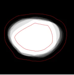
By doing this for a set of atlases we obtain a good initial guess of where the pericardium is spatially (see Figure 1.2). These registrations will be done in two parts. Firstly, an affine (rigid) transformation will be estimated. Sec-ondly, that affine transformation will be used as an initialization for a non-rigid transformation based on B-splines.
Since image registrations can be very time consuming we propose to base the multi-atlas segmentation on feature based registration (specifically SURF, Speeded Up Robust Features [1]). Feature based registration is a lot faster than more widely used (in medical image analysis) intensity based registration methods. It is not used much since medical images produce a lot of outliers.
1.3. PROPOSED SOLUTION
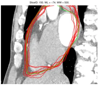
SliceID: 150. WL = −74. WW = 500.
Figure 1.2: A sagittal slice of one of the atlases. By aligning the labels of several atlases (by estimating a transformation through registration) onto the target image we get a good estimate of the segmentation. Each red line in this figure represents the boundary of an aligned labeling using feature based non-linear registration. The green line corresponds to the boundary of the gold standard (the manual labeling).
But we propose to handle the outliers mainly using Random Sample Consesus (RANSAC), [9]. To evaluate this method we compare the results with Niftyreg which is an intensity based method used widely for medical registration.
The problem remains on how to decide on a final segmentation given the guesses (votes) from the atlas registrations. The most straight forward way is to include all voxels which half or more of the atlases label as inside the pericardium. This is called majority voting (or decision fusion). Sometimes the feature based registration makes mistakes that are obvious when looking at the specific intensities of the voxels. For example, this can happen if lung cavity is included in the segmentation In Figure 1.2 you can see this e↵ect where some of the red lines pass through the lung meaning that some of the atlases estimate the lung to be inside of the pericardium. These types of errors are easily corrected by incorporating the votes into a Markov Random Field (MRF) (see e.g. [4]) together with the intensity information. The MRF has two main advantages. It is very flexible in the sense that it is easy to incorporate di↵erent information and it can be optimized in polynomial time by representing the MRF as a graph and finding the minimal cut through the graph using maxflow algorithms.
The MRF in its most used formulation only regularizes the boundary making the segmentation surface smooth. We propose an extended formulation that makes the cost of the boundary data dependent, actively pushing the boundary towards a probable path. In this work we only use pixel intensity and the number of multi-atlas votes as observations on which we build the MRF but the framework is easily expandable to more complex features and classifiers.
CHAPTER 1. INTRODUCTION
1.4
Contributions and Related Work
Recently a few methods have been developed for fully automated pericardium segmentation. In [19] Shahzad et al. use multi-atlas segmentation with major-ity voting. Practically the same method as was used by Kirisly et al. [11] for cardiac segmentation. Both algorithms were based on intensity based registra-tion (Elastix). Dey et al. [7] used another intensity based registraregistra-tion algorithm (Demons) and proposed to speed up the the segmentation time by co-registering the atlases before hand and given an unlabeled image only performing one atlas registration. By measuring the di↵erence between each atlas and the target image a weight was calculated measuring the importance of the atlas for the decision fusion.
The contributions made by this work is partly that feature based registration works excellent for registration of medical images and at huge gain in compu-tational efficiency. Especially we show that feature based registration proves considerably more accurate and robust for initialization of the nonrigid reg-istrations compared to the computationally more demanding intensity based algorithm Niftyreg. We also propose an efficient algorithm for pericardium segmentation based on feature based multi-atlas segmentation that shows sig-nificantly improved results over previous state-of-the-art-methods.
1.5
Structure of the Report
In Chapter 2 we explain the theory that is needed to follow the what is covered in this report. The problem of image registration (Section 2.1) Markov Random Fields (Section 2.2) and graph cuts (Section 2.3) are explained. Everything in this chapter is frequently used notions in image analysis and computer vision and can be skipped if the reader already is familiar with these terms. The method is divided into two parts. In Chapter 3 we begin by presenting multi-atlas segmentation in general. We continue with presenting two di↵erent registration methods that we evaluate as basis for the multi-atlas segmentation. One feature based using SURF, Lowe matching and RANSAC (Section 3.1) and one intensity based using Niftyreg (Section 3.2). In Chapter 4 we present our method for fusing the votes from the multi-atlas registrations into a final segmentation by optimizing an MRF through graph cuts. In Chapter 5 we cover all the details of the implementation that is needed for reproducibility (e.g. di↵erent settings and parameters). Thereafter (in Chapter 6) we present the results where we evaluate the di↵erent steps of the algorithm. The results are discussed in Chapter 7 and lastly we present the conclusion in Chapter 8.
Chapter 2
Theory
In this chapter we will cover some theory that the reader needs to be famil-iar with to be able to follow the rest of this report. Firstly, the problem of image registration and two types of widely used transformations that we will use in this work (affine transformation and non-rigid transformation based on B-splines) will be explained. Using our knowledge of registration we can then proceed to explain multi-atlas segmentation. After that the theory of Markov Random fields will be presented and a way to formulate the problem of finding the maximum a posteriori probability of this Markov Random Field by finding the minimal cut, or equivalently maximal flow, through a graph (often referred to as graph cuts).
2.1
Image Registration
This section covers the basics of image registration. For further information see for example [10, 25, 20].
2.1.1
Problem Formulation
Image registration is the process of spatially aligning two images, i.e. finding a one-to-one map between one image and another so that the corresponding points in the images refer to the same point in the object they are depicting. Formally this can be formulated as:
Given atarget imageIt(also in the literature referred to as reference or static image) and asource imageIs(floating or moving image), find the values of the parameters ✓of the transformation (mapping function)T(✓) that minimizes a cost function⇢, i.e.
arg min ✓
(⇢(It,T(✓) Is)) (2.1)
where the cost function ⇢is a measure of the accuracy of the registration, i.e. the similarity between the target image and the transformed source image.
2.1.2
Transformations
There are many ways to define the mapping function T. You want to have a transformation model that describes the real expected transformation between
CHAPTER 2. THEORY
the source and target images as accurately as possible. At the same time you do not want the model to be too complex. If the model has a lot of parameters not only will the optimization be computationally more demanding, it will also be harder to optimize.
To try and avoid the problem of finding local minima the problem is usually split into two parts. The first part is a rough registration with a simpleraffine transformation. Since the affine transformation is easier to optimize we use that as an initialization for the second part, which is a more complex free-form deformation which allows for local deformations in the image.
Affine Transformation
The affine transformation (here denotedTa↵) is a composition of a translation
and a linear map and can be represented by a 4⇥4-matrix with 12 parameters (✓=✓1, . . . ,✓12) and can be described by
Ta↵(✓) = 2 6 6 4 ✓1 ✓4 ✓7 ✓10 ✓2 ✓5 ✓8 ✓11 ✓3 ✓6 ✓9 ✓12 0 0 0 1 3 7 7 5 (2.2)
for each voxel the transformation is then defined by y 1 =Ta↵(✓) x 1 (2.3)
where x is the voxel coordinates in the source image and y is the new trans-formed coordinates.
The intensity based registration method that we evaluate estimate an affine transformation. But the feature based method for efficiency estimates a rigid transformation. A rigid transformation is a special case of an affine transforma-tion which only allows for rotatransforma-tion and translatransforma-tion and the number of degrees of freedom are reduced to 6.
Free-Form Deformation
The affine transformation is a global transformation but the anatomical struc-ture of the hearts that we will try to register will display more complex relations. This means that we need a transformation that also can handle local deforma-tions. In this work we will be using two methods which both use a free-form deformation (FFD) model based on cubic B-splines. The method is by Rueckert et al. from 1999 [18]. FFD is a method which has got wide acceptance in the medical image analysis community [20].
A grid of control points is superimposed on the image and the basic idea is that the image will be influenced by manipulating the control points. The control points control the B-splines and the resulting deformation will be a smoothC2 continuous transformation. Another advantage of B-splines is that they have local support, i.e. a control point will only influence a local region around that control point which makes the transformation easier to optimize and compute.
2.2. MARKOV RANDOM FIELDS
To mathematically formulate the FFD (following the formulation in [18]) we define the domain of the (in our case 3D) image as
⌦={(x, y, z)|0x < X,0y < Y,0z < Z}
whereX,Y andZdefine the size of the image. Annx⇥ny⇥nzgrid of uniformly spaced control points✓i,j,kis superimposed on the image. By moving the control points the image is transformed which means that the set of parameters is the position of these points. The transformation of a pointx= (x, y, z) is defined as T↵d(✓) x= 3 X l=0 3 X m=0 3 X n=0 Bl(u)Bm(v)Bn(w)✓i+l,j+m,k+n (2.4) where i = bx/nxc 1, j =by/nyc 1, k =bz/nzc 1, u= x/nx bx/nxc,
v=y/ny by/nyc,w=z/nz bz/nzcandBlrepresents the l:th basis function of the B-spline, i.e.
B0(u) = (1 u)3/6
B1(u) = (3u3 6u2+ 4)/6
B2(u) = ( 3u3+ 3u2+ 3u+ 1)/6
B3(u) =u3/6.
If you have a 10⇥10⇥10 grid of control points there are 3000 parameters that need to be optimized but as is clear from (2.4) the transformation of xis only dependent of the location of the 27 closest control points. This means that if you move any of the other control points it will not a↵ect this part of the image and hence the support for the control points is local which makes the parameters easier to optimize.
For a deeper read about B-Splines in general see for example [5]. For a comparison with other methods see [20].
2.2
Markov Random Fields
Probabilistic graphical models combine knowledge from probability theory and graph theory and are a powerful formalism for a wide range of problems in various scientific fields. In computer vision (and other fields) one especially powerful method is regarding the image as originating from a Markov Random Field (MRF), partially because it can model the underlying quantity to be smooth (which is often the case in computer vision) and because it is very adaptive and can handle a wide variety of priors. If the MRF is formulated in a sensible way it can be formulated as a graph and the maximum a posteriori distribution can be found using graph cuts, i.e. it can be globally optimized in polynomial time.
Following the notation in [4], you have a set P = {1, . . . , m} of sites p
(pixels/voxels). You have a neighborhood systemN ={Np|p2P}whereNp is the set of pixels that are considered neighbors topand a field (set) of random variablesF ={Fp|p2P}where each random variable Fp can take a valuefp in some set of labels. A joint event {Fp =fp|p2P} is abbreviated F = f where f ={fp|p2P} is a realization (or configuration) of the random field.
CHAPTER 2. THEORY
In the context of segmentation the optimal configuration will be used directly as labels describing the final segmentation (i.e.fp=lp). For now we choose to
separate the notation betweenfp (meaning a realization of the random variable
Fp) and lp (representing the label of a voxel in an image). We will abbreviate
Pr(F =f) as Pr(f) and Pr(Fp=fp) as Pr(fp). An MRF is a fieldF with the
property (known as local Markov property) that each random variableFp only
depends on its neighbors
Pr(fp|fP\{p}) = Pr(fp|fNp), 8p2P. (2.5)
According to the Hammersley-Cli↵ord theorem any distribution that obeys the Markov property (2.5) can be written as
Pr(f)/Y c2C exp ( Vc(fc)) = exp X c2C Vc(fc) ! (2.6) where C is the set of all maximal cliques of the MRF. A clique is a subset of variables that are all connected to each other. Vc is called the potential
function of the clique c and is a positive real-valued function on the possible configurations fc of the clique. In this work we will only consider the pairwise
MRF in which the probability in (2.6) is factorized into potential functions defined on cliques of size strictly less than three. Although the MRF can always be defined by potential functions on the maximal cliquesCusually the potential function is split onto set of unary potentials Vp which are defined on single
variables and a set of pairwise potentials Vp,q which are defined on pairs of
variables. The probability of a configuration can then be written
Pr(f)/exp 0 @ X p2P Vp(fp) X {p,q}2N V{p,q}(fp, fq) 1 A. (2.7)
The realization of the field f is generally not observed directly so it needs to be estimated through the joint event O = {Op=op|p2P} referred to
as the observation. In computer vision the realization op can for example be
the observed intensity at the pixel p. In this work the observation will be a combination of the intensities in the image and vote map from the multi-atlas segmentation. The probability that we are interested in is the posterior probability Pr(f|O) which can be defined straight forwardly as
Pr(f|O)/exp 0 @ X p2P Vp(fp;op) X {p,p}2N V{p,q}(fp, fq;op, oq) 1 A. (2.8) We are interested in finding the configurationf that maximizes the posterior probability (2.8). Since the logarithm is a monotonically decreasing function maximizing the posterior probability is the same as minimizing the posterior energy function E(f) = ln(P(f|O)) =X p2P Vp(fp;op) + X (p,q)2N V{p,q}(fp, fq;op, oq) (2.9)
2.3. GRAPH CUTS
Of course this energy can be rewritten as functions on the maximal cliques
E(f) =X
c2C
Vc(fp, fq;op, oq). (2.10) For more on MRFs see for example [22] and [21].
2.3
Graph Cuts
2.3.1
Problem Formulation
Consider a weighted graph G =hV,Ei consisting of a set of n nodes V and a set ofmedgesE where each edge e2E in the graph has a nonnegative weight (or cost)we. Define two special nodes, usually referred to asterminal nodes or source sand sink t nodes (there can be more than two terminal nodes but in this work we will consider the binary problem). Acut through the graph is as a subset of edgesC⇢E such that in the graphhV,E\Cithe terminal nodes are separated, i.e. there are no path fromstotwhen the edgesCare removed from the graph. The graph is partitioned into two completely separated graphs. The graph cut problem (also called min-cut/max-flow problem for reasons that will be clear in a moment) is to find the minimal cut, i.e. find the cutCthrough the graphG such that the sum of the cost of the edges that are cut is minimal
arg min
C⇢E X e2C
we. (2.11)
According to one of the fundamental theorems of combinatorial optimization by Ford-Fulkerson the min-cut problem is dual to the max-flow problem. The max-flow problem is easily understood by considering the edges of the graph as pipes and the costs of the edges is the capacities of the pipes (i.e. the amount of flow they can facilitate) the problem is now stated as the maximum flow (of e.g. water) that can be pushed from the source to the sink. When the maximum flow is found some pipes will be saturated and the set of saturated pipes will be equal to the minimum cut. The realization that the min-cut problem and the max-flow problem are dual is important since the max-flow problem can be solved in polynomial time by di↵erent algorithms that iteratively push flow through the edges until the saturated state is achieved. For reference see for example [3].
2.3.2
Graph Cuts in Computer Vision
To reformulate an image as a graph G, let each pixel/voxel p be a node. A neighborhood systemN is defined by putting an edge (p, q) between each pair of neighboring voxels p and q. Define two extra nodes s and t and connect edges froms to each of pand from eachpto t. The edges between the pixels are usually referred to asn-links(for neighborhood) and the edges between the pixels and the terminalssandt are calledt-links. All of the edges are assigned weightswe. For a small 3⇥3 example image the graph will look like Figure 2.1. To build some intuition about this graph we consider a cut through the graph separating s andt. We define the set S ⇢P as the set of nodes connected to
CHAPTER 2. THEORY
Figure 2.1: The grey nodes represent a 3⇥3 image. the nodes are connected to its neighbors and all pixels are connected both to the source nodesand the sink nodet. All edges have costswe. The cut parts the graph so that no path
exists betweensandtand the pixels are separated into two sets: the pixels that are connected tos and the pixels that are connected tot. The minimal cut is the cut that separatestandsand has the minimal cost. Figure is found in [3].
to the setS it will be labeled asfp = 1 (foreground) andfp= 0 (background)
if it belongs to T. In fact we view the graph as describing a second degree pseudo-boolean function, i.e. a function from the boolean configurations of the nodes (fp2{0,1}) toRthat can be factorized into
E(f) = X 8{p,q}
a(fp, fq). (2.12)
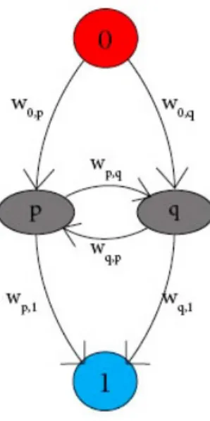
To understand this we look at a small example 2.2. Each edge in the two-node graph has a weight. We want to cut the graph into two parts where the nodes connected to 0 will be labeled 0 and the nodes connected to 1 will be labeled 1. We have four possible configurations of this graph. If we want to label
fp = 1 and fq = 0 the edges w0,q, wp,1 and wp,q are cut and the cost of this
configuration hence isa(1,0) =w0,q+wp,1+wp,q. In the same way we define
costs for the other configurationa(0,0),a(0.1), a(1,1).
Now propose that se defined the costsa of the di↵erent configurations and we want to set the weights w so that the graph describes these costs. One formulation is
wp,0=a(1,0) a(0,0) w1,p=a(1,0) a(1,1)
w0,p=a(1,0) +a(0,1) a(0,0) a(1,1)
and setting the rest of the weights to 0. By this convention we can formulate a graph that describes any quadratic pseudo-boolean function where we have defined the cost of a configuration of each clique {p, q} as a{p,q}(fp, fq). If we
want the function to be easily optimized there is the criterion that all weights
win the graph must be non-negative. This is achieved if the following criterion onaholds (referred to as submodularity):
2.3. GRAPH CUTS
Figure 2.2: The grey nodes represent a small two node graph. Both nodes are connected to each other and the source (denoted as 0) and the sink (denoted as 1). All edges have defined weightswe.
Now we note that the energy function describing the MRF (2.11) is a quadratic pseudo-boolean function. This of course means that the energy function can be represented by a graph and as long as it is submodular (which it turns out to be in our formulation) it can be formulated as graph with non-negative weights and the minimal cut of the graph corresponds to the configurationf that maximizes the posterior probability (2.8) of the MRF. For further information see [2].
Chapter 3
Method: Multi-atlas
Segmentation
Multi-atlas segmentation is a method that has become very popular for many di↵erent medical applications, including segmenting brain and its internal struc-tures, lungs, hearts and other internal abdominal organs [8].
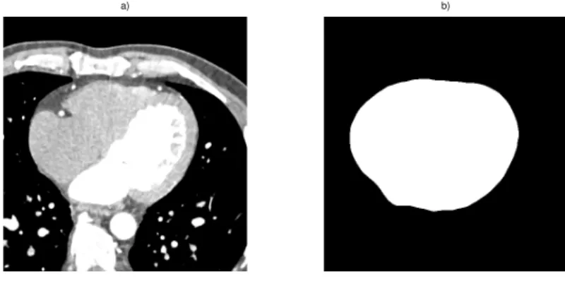
An anatomicalatlasis an imageI={ip|p2P}with corresponding manual labelingL ={lp | p2P}. In our case we have a CT-volume of a heart and a binary volume of equal size with the labeling done by an expert. If a voxel p
in the binary volume has value 1 it means that lp = 1 andip describes a part of the image that is inside the pericardium (foreground). Iflp= 0, ip describes a part of the image that is outside of the pericardium (background). I and L together will be referred to as an atlas. An example slice of one of our atlases can be seen in Figure 3.1.
a) b)
Figure 3.1: a) One slice of an CT-volume. b) Corresponding slice of the manual labeling. Together a) and b) form an atlas.
When given a new unlabeled target imageIt an atlas imageIsis registered to the target image and a transformation Tis estimated. This transformation should align the source image onto the target image. By applying the same transformation on the labeled volumeLs, the labels should also align onto the
3.1. FEATURE BASED REGISTRATION
target image. This is called label propagation and can be used as a labeling (segmentation) of the voxels of the target image. The process of registering an atlas to a target image and segmenting the image through label propagation is called single-atlas segmentation.
Multi-atlas segmentation registers multiple atlases to the target image and then combines their segmentation labels. Because of the natural variation e.g. between di↵erent hearts, one single atlas might fail to accurately classify the target image. Using multiple independent classifiers and fusing their results might produce better results.
There are several ways of combining the labels into a final segmentation. The most straight forward is majority voting (also referred to as decision fusion or label voting). Each atlas labeling is considered a vote. The label of a voxel in the target image is selected as the label that a majority of the atlas segmentations agree on. Majority voting will be used to evaluate the multi-atlas segmentation based on the di↵erent registration techniques. But the final segmentation will be found by incorporating the multi-atlas votes into an MRF field and finding the maximum a posteriori configuration through graph cuts (explained in Chapter 4).
Multi-atlas segmentation is at its core multiple image registrations. There are a lot of proposed methods for solving the registration problem described in Section 2.1. In this work we choose to evaluate the performance of two di↵erent methods. Onefeature basedand oneintensity based method. The feature based methods in general di↵er from the intensity based methods in that they, instead of directly working with the intensity levels of the pixel/voxel, extract features that represent the information of the image on a higher level. The problem reduces to registering the extracted features in the images to each other.
Feature based registration methods are usually recommended when the im-ages contain enough distinctive and easily detectable objects as is often the case in many areas of computer vision. In medical images on the other hand, the objects are often not as rich in detail. Features can be extracted but a large amount of them will be noise or mismatched between the images and hence result in a lot of outliers when the transformation between the images is es-timated. Because of this drawback feature based methods are rarely used in medical applications, see [25].
However, since we are interested in making multiple registrations for each new patient for the multi-atlas segmentation and since ultimately this work is supposed to be used on a very large data set (in connection with the SCAPIS project), it is of value if we can make it less computationally demanding and feature based registration is in general much faster to compute. Therefore we evaluate two methods. One feature based method based on SURF and one intensity based method named Niftyreg.
For more about registration and the di↵erent methods see for example [25, 20].
3.1
Feature Based Registration
The feature based registration method that we use is based on SURF [1]. SURF has shown to outperform comparable methods not only in speed but also in robustness, i.e. it is less sensitive to noise [1]. This is valuable to us since we are
CHAPTER 3. METHOD: MULTI-ATLAS SEGMENTATION
dealing with a lot of outliers. To further try to cope with the outlier problem we use RANSAC, which is very robust to outliers, to estimate the transformation between the features obtained from SURF.
The registration uses SURF for feature detection and feature description, the matching criterion by Lowe to find correspondences between the detected fea-tures and RANSAC to estimate a rigid transformation between the two feature sets. Finally, a B-spline based transformation is used to map the correspon-dences even closer to each other.
3.1.1
SURF
Speeded-Up Robust Features (SURF) is a method for feature detection and de-scription developed by Herbert Bay et al. in 2006 [1]. It was originally developed for images in two dimensions (and so will this explanation be) but the concept is easily expandable to 3D. It consists of two parts: interest point detection and interest point description.
Interest Point Detection
Interest points are points in the image that seem more like the center of a blob than points in its neighborhood. The detection of these points is based on approximation of the determinant of the Hessian matrix which describes the curvature of the image. The Hessian matrixH(x, ) of a point xat scale is given by
H(x, ) =
Lxx(x, ) Lxy(x, )
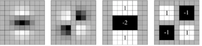
Lxy(x, ) Lyy(x, ) (3.1) whereLxx(x, ) is the convolution of the Gaussian second order partial deriva-tive @@x22g( ) with the image I at x and similarly for Lxy and Lyy. If the
determinant is large, the blob response is high and if the blob response is higher than the blob response in a neighborhood (local maxima) the point is detected as an interest point. This detection is done for di↵erent scales with di↵erent sizes of the convolution filters to be able to detect blobs of di↵erent sizes. The scale space is divided into octaves (representing an scaling factor of 2) and each octave is subdivided into a constant number of scales.
The Hessian has been used before as a way to detect interest points but Bay et al. proposed to speed up these calculations by approximating the convolu-tion filtersL with simple box filters (see fig 3.2) which can be calculated very efficiently with use of the integral image. The element at x = (x, y)| in the integral imageI⌃relates to the original imageI as
I⌃(x) = ix X i=0 jy X j=0 I(i, j). (3.2)
This conversion allows for efficient computation of the sum of all pixel in-tensities in any upright rectangular area since, regardless of size, it only needs to evaluate four points inI⌃(see fig 3.3).
3.1. FEATURE BASED REGISTRATION
Figure 3.2: From left to right: the discretized second order partial derivative iny- (Lyy) andxy-direction (Lxy), respectively. And the box approximation of these filters.
Figure 3.3: To evaluate the sum of all pixels ⌃ inside a box you only need to evaluate and sum four elements in the integral imageI⌃
Interest Point Description
To be able to successfully match an interest point in one image to the corre-sponding feature in another image, each interest point is described with a vector (a descriptor). The descriptor should be invariant to the transformations that are expected between one image and the other. If that is the case the descrip-tors of corresponding points in the di↵erent images would be similar and the euclidean distance between these descriptors would be small.
The description of the features uses information from the interest points neighborhood. Firstly, in order for the descriptor to be rotation invariant, a reproducible orientation for the image point is identified. This is done by cal-culating the Haar wavelet (see Figure 3.4) responses in x and y direction in a circular neighborhood around the point. Both the radius of the neighborhood and the size of the Haar wavelets are scaled according to in which scale the in-terest point was detected to make the descriptor scale invariant. The response from the wavelets in the x and y direction are then used to find a dominant orientation of the neighborhood.
To extract the descriptor, a square region centered at the interest point and oriented along the dominant orientation is constructed. The size of this region is again dependent of the scale. This region is divided into 4⇥4 sub-regions and for each of these subsub-regions the x and y Haar wavelet responses are evaluated at the points of a 5⇥5 grid inside the subregion. The responses in the horisontal direction (perpendicular to the dominant direction) are here denoted dx and the the responses in the vertical direction are denoteddy, the
CHAPTER 3. METHOD: MULTI-ATLAS SEGMENTATION
Figure 3.4: Haar wavelet filters in thex- andydirections. Dark areas has weight 1 and white has weight +1.
intensity structure of that subregion is described by a 4D-description vector
v = (Pdx,Pdy,P|dx|,P|dy|). Concatenating these from all subregions of
the interest point you get a final feature descriptor of length 64.
3.1.2
Matching
For each image (the target and the source) a set of features are extracted. The next step is determining which features in the source set that are corresponding to which features in the target set. The most straight forward way would be to find the feature that is closest (in the descriptor space). However only choosing correspondences by which features have the most similar descriptors will result in a lot of bad matches. A more e↵ective method (as shown by Lowe [13]) is to compare the closest neighbor to its second closest neighbor. Two features are matched if the ratio between the distance between a features closest neighbor and its second closest is below a certain threshold. I.e. if the descriptor vector is denotedd,d1is the closest feature todandd2is the second closest, a match
is found if
|0d d1|0
|0d d2|0
⇢ (3.3)
where⇢is a parameter. In other words a match is found if a feature has a match that is considerably closer than any other match. The matches are in this work found by exhaustive search.
As mentioned earlier, medical images are not very rich in detail which results in there not being many distinct features. If the the matching threshold⇢is set to low we might end up with too few matches to be able to estimate a reliable transformation. Instead we set⇢high, resulting in a larger amount of matches but also more outliers.
3.1.3
RANSAC
Given the correspondences found from the matching in Section 3.1.2 we want to find a transformation that transforms the points in the source image onto the points in the target image. This is done using RANSAC, a method which is very insensitive to outliers.
Random Sample Consesus (or RANSAC) is a method developed in 1981 by Fischler and Bolles [9] for fitting a model to experimental data. Fischler and Bolles recognized that there are two types of errors present in experimental
3.2. INTENSITY BASED REGISTRATION
data, classification and measurement errors. Classification errors are outliers that are not captured by the model (e.g. when the detector incorrectly identifies a feature). Measurement errors occur when the detector correctly identifies a feature but slightly miscalculates one of its parameters (usually modeled by a normal distribution). Standard fitting techniques like least squares will fail since the gross classification errors will have a significantly larger e↵ect than the measurement errors and the errors will not balance out.
RANSAC handles this by, instead of using all of the data for parameter estimation, randomly selects a minimum set of features and uses these to esti-mate the parameters of the transformation. Given these estiesti-mated parameters, find the set of features (the consensus set) that are within some error threshold of this model and therefore can be considered measurement errors. Iteratively redo these calculations for new randomly chosen initialization sets and choose the parameters of the model with the largest consensus set (i.e. the model with the most inliers).
We were trying to estimate a rigid transformation T(✓) which has 6 pa-rameters. The minimal random set hence consists of 6 correspondences (6 points x = (x1, . . . , x6) in the source image and their corresponding points y= (y1, . . . , y6) in the target image). The transformation relating these points
to each other are easily computed explicitly so that
y=T(✓) x. (3.4) Now map all points in the source image with this transformation and count the number of points that are transformed within a threshold distance from its corresponding point in the target image (i.e. the number of correspondences in the consensus set).
3.1.4
B-spline registration
The correspondences found by RANSAC are mapped to each other non-rigidly using a package developed by Dirk-Jan Kroon available freely for MATLAB called B-spline Grid, Image and Point based Registration. It contains a point based B-spline registration based on the paper by Lee et al. [12]. It estimates a B-spline based free form deformation that maps corresponding points onto each other analogously with the intensity based free form deformation in the Niftyreg package that will be explained in Section 3.2.
3.2
Intensity Based Registration
Niftyreg is a freely available medical image registration package. It contains two programs for image registration that we are using in this work, reg aladin
and Reg f3d. Reg aladin estimates an affine/rigid transformation and is based on block-matching. Reg f3dcomputes a free form transformation based on B-splines.
Reg aladin
The algorithm, on which Reg aladinis based, was presented in [16] and [17] by Ourselin et al. Basically, the source image is divided into blocks B0 and each
CHAPTER 3. METHOD: MULTI-ATLAS SEGMENTATION
of these blocks is compared to blocks in the target image B. The similarity between a block Bab0 centered at (a, b) in the source image and a block Buv
centered at (u, v) in the target image is measured using the normalized cross correlation of the blocks
C(Bab,Buv) = 1 N2 NX1 i=0 NX1 j=0 Is(a+i, b+j) µs(a,b) It(u+i, v+j) µs(u,v) s(a,b) t(u,v) (3.5) whereµs(a,b) and s(a,b) is the mean and standard deviation of the blockBabin
the source image and µt(u,v) and t(u,v) is mean and standard deviation of the
block Buv in the target image. To reduce computational time only the blocks
with high variability ,which correspond to high contrast regions, are considered. The block matching provides a set of corresponding points (the centers of the best matching blocks). Ourselin et al. estimates that 20% of the obtained matches are due to outliers and notes that the least squares approach to es-timating the parameters ✓ of the affine transformation Ta↵ is unsatisfactory.
Instead they propose to use the L1-estimator. That is find the transformation
that minimizes the sum of theL1 norm of the residuals rk =yk T, in other
words, minimizes Pk|rk|. Since it is a slower growing function than the L2
norm it is less sensitive to outliers. Ultimately they ended up using the man-hattan distance of the residual instead of the euclidean distance. Although the manhattan distance is dependent of the particular coordinate system Ourselin et al. observe that it yields slightly better results compared to the Euclidean distance.
The source image is transformed using the estimated transform and then the block matching starts over, iteratively updating the transform until the variation between the new transform and the previous one gets small enough or a set number of iterations. Because of the complexity of the algorithm it uses a multi-scale implementation where it first finds a rough transform at a coarse scale. When the a transform is found it continues but on a refined scale. The algorithm stops when the block size becomes so small that the information of the block is considered insufficient or after a set number of levels.
Reg f3d
Reg f3d is based on an algorithm presented by Rueckert et al. [18] and the implementation is by Modat et al. and described in [14]. The algorithm seeks to minimize a cost functionC associated with the control points of the B-spline grid (which were covered in Section 2.1.2)
C( ) = Csimilarity(It,T(Is)) + Csmooth(T). (3.6)
The first term measures the similarity between the target image It and the
transformed source imageIsusing normalized mutual information (NMI).
Mu-tual information is a concept from information theory and measures how much of the information in one imageAis present in the other imageB. More specif-ically
Csimilarity(A, B) =H(A) +H(B) H(A, B) (3.7)
whereH(A) andH(B) are the marginal entropy ofAandBandH(A, B) is the joint entropy. These are calculated by computing estimations of the histograms of the voxels in the images.
3.2. INTENSITY BASED REGISTRATION
The second term describes the smoothness of the transform. Since, in gen-eral, we know that the transformation will be smooth we can penalize the trans-formation for bending to much by adding the bending energy of the transfor-mation to the cost function
Csmooth= 1 V Z X 0 Z Y 0 Z Z 0 ✓@2T @x2 ◆ + ✓@2T @y2 ◆ + ✓@2T @z2 ◆ + + ✓@2T @xy ◆ + ✓@2T @xz ◆ + ✓@2T @yz ◆ dxdydz (3.8)
The transformation is optimized with a multi-scale approach where the spac-ing between the control points initially are large (i.e. there are fewer parameters for the transformation and the possible transformations are on a more global level). To find the optimal position for the control points the conjugate gradi-ent descgradi-ent method is used where the gradigradi-ent of the cost function is estimated and iteratively a step proportional to the length of the gradient vector is taken downwards. When a local optima is found (the length of the gradient gets be-low a threshold) more control points are added which albe-lows for a more local transformation and the optimization starts over.
Chapter 4
Method: MRF
Segmentation
There are many di↵erent segmentation techniques. This work is focused around multi-atlas segmentation which is based on multiple image registrations (which was covered in chapter 3)
However, the multi-atlas segmentation will never be perfect. Especially the feature based method, which works with the images on a higher level (register-ing extracted features to each other) and with data with a lot of outliers, will sometimes produce errors which are apparent when taking into consideration the intensity information (e.g. when lung tissue is classified as inside the peri-cardium). Therefore we constructed an MRF into which we could incorporate both the atlas registrations and the intensity information. Another advantage of the MRF formulation (apart from being very flexible) is that it can be globally optimized in polynomial time using graph cuts.
4.1
MRF Formulation
What is usually done (for e.g. in [4]) is rewriting the posterior probability using Bayes’ Theorem as
Pr(f|O) =Pr(O|f) Pr(f)
Pr(O) /Pr(O|f) Pr(f) (4.1) where the likelihood Pr(O|f) is assumed to factorize as
Pr(O|f) =Y p2P
Pr(op|fp) (4.2)
i.e. each Pr(op|fp) is independent of the rest of the field. Here f on the other hand is assumed to be a Markov field and according to Hammersley-Cli↵ord (see Section 2.2) it factorizes to
Pr(f)/exp 0 @ X {p,q}2C Vp,q(fp, fq) 1 A. (4.3)
4.1. MRF FORMULATION
Thepairwise clique potential V{p,q} is usually set to
Vp,q(fp, fq) = ⇢
, fp6=fq
0, fp=fq (4.4)
where is a constant which regularizes the segmentation by penalizing making the boundary of the segmentation too long.
Of course, saying that f is a Markov random field, and that the likelihood Pr(O|f) is not, is only a trick to divided the problem into parts that are easier to understand intuitively. We can rewrite Pr(f|O) into a product of functions a{p,q}(fp, fq) on the maximal cliques {p, q} by collecting (4.2), (4.3) and (4.4) into Pr(f|O)/exp 0 @ X {p,q}2C a{p,q}(fp, fq) 1 A, (4.5) where a{p,q}(fp, fq) = ⇢ ln(Pr(op, oq|fp, fq)), fp=fq ln(Pr(op, oq|fp, fq)) + , fp6=fq . (4.6) (4.5) and (4.6) represent the same MRF as above (apart from a constant that is dependent on the number of neighbors to each pixelp) and both are maximized by the same configurationf. This formulation will be referred to as theoriginal formulation.
4.1.1
Expanding the formulation
Formulating the probability as in the original formulation has two main ad-vantages: it is an easy formulation and it regularizes the segmentation in a predictable way which means that you have some control over the shape of the segmentation. The main disadvantage is that, for it to work satisfactory, the boundary cannot pass through an area where there is an overlap between the density functions Pr(op|Fp = 0) and Pr(op|Fp= 1). If it is, the location of the boundary will be ambiguous and the regularization will fall back to the shortest path.
Segmenting the pericardium su↵ers from this drawback. If the pericardium is located directly between the lung cavity and the myocardium the classification is straight forward since the air is clearly not inside and the probability of the soft tissue that constitutes the myocardium is rather likely to be inside. In theses areas the segmentation using the MRF will show a clear improvement over the multi-atlas segmentation. But the pericardium often passes through fat tissue. Fat is likely to be found both outside and inside of the pericardium and in these areas the multi-atlas segmentation is not likely to be improved by the MRF.
But there are some indicators of where the boundary should be since the pericardium is not completely invisible. We want to exploit this fact by making the cost of the boundary dependent on these observations and we propose to find a simple and intuitive formulation that can guide the boundary in areas of ambiguity. We have been experimenting with a lot of di↵erent functions for the cost of the boundary which all have in common that they are a function of the negative logarithm of some probability that is dependent on the observa-tions. We tried a large set of formulations but found the following to be not to complicated and at the same time work well on our training sets.
CHAPTER 4. METHOD: MRF SEGMENTATION
The Hammersley-Cli↵ord Theorem (see Section 2.2) states that Pr(f|O)/exp 0 @ X {p,q}2C V{p,q}(fp, fq) 1 A.
Since the probability factorizes over the cliques we can split the formulation onto the setsf==
{{p, q}2N |fp=fq}andf=6 ={{p, q}2N |fp6=fq}and we get Pr(f|O)/exp 0 @ X {p,q}2f= V{p,q}(fp, fq) 1 Aexp 0 @ X {p,q}2f6= V{p,q}(fp, fq) 1 A /Pr(f= |O) Pr(f6=|O). (4.7) Pr(f=
|O) will be written straight forwardly as Pr(f=|O)/ Y
{p,q}2f=
Pr(fp, fq|op, oq) (4.8)
which corresponds to a potential function
V{p,q}(fp, fq) = ln(Pr(fp, fq|op, oq)), fp=fq.
Here it is worth noting that all probabilities regarding specific pixels are con-sidered independent of all other pixels. For example we have
Pr(fp, fq|op, oq) = Pr(fp|op) Pr(fp|op) = Pr(op|fp) Pr(fp) Pr(op) Pr(oq|fq) Pr(fq) Pr(oq) . (4.9) Pr(f6=
|O) describes the probability of the boundary and we put a little more thought into formulating this probability. We want to construct a modified probability distributiong(fp, fq;op, oq) that gives us some control over the cost
of the boundary.
In the original formulationg was simply formulated as g(fp, fq;op, oq) = Pr(fp, fq|op, oq).
But now we see thatgshould also reflect the probability offp andfq belonging
tof6=. We let
Bbe the set of pixels that are on the boundary, i.e.B={p2P | p2f6=
}. A more natural formulation ofg then is
g(fp, fq;op, oq) = Pr(fp, p2(B)|op) Pr(fq, q2B|op) (4.10)
and we can rewrite this as
g(fp, fq;op, oq) = Pr(p2B|fp, op) Pr(q2B|fq, op) Pr(fp, fq|op, oq).
We denotegb(fp, fq;op, oq) = Pr(p2(B)|fp, op) Pr(q2B|fq, op) which gives us
Pr(f=|O)/exp 0 @ X {p,q}2f6= ln(g(fp, fq;op, oq)) 1 A = exp 0 @ X {p,q}2f6= ( ln(Pr(fp, fq|op, oq)) ln(gb(fp, fq;op, oq))) 1 A. (4.11)
4.1. MRF FORMULATION
Now we can collect (4.8) and (4.11) into (4.7) and get Pr(f|O)/Pr(f=|O) Pr(f6=|O) = exp 0 @ X {p,q}2C ln(Pr(fp, fq|op, oq)) 1 APr(B|f,O) (4.12) where Pr(B|f,O) = exp 0 @ X {p,q}2f6= ln(gb(fp, fq;op, oq)) 1 A .
We note that if gb equals a constant we have the original formulation which simply regularizes the segmentation. If we estimate the probabilities in gb we get a cost of the boundary that in a natural way reflects the probability of the boundary given the observations.
We further introduce two parameters 1 and 2 to control the e↵ect the
boundary cost will have on the segmentation Pr(B|f,O) = exp 0 @ X {p,q}2f6= 1ln(gb(fp, fq;op, oq)) + 2 1 A (4.13) Finally, we set
1ln(gb(fp, fq;op, oq) + 2= 3, 8op, oq 2/fat (4.14)
where 3 is some constant. This is done to isolate the peak ingb which actually
corresponds to the intensities found on the pericardium when it is visible. If the observations tell us that the current pand q are fat we will look for the most probable path through the fat. Ifporqare not fat,gb is set to a constant and we are instead falling back to regular regularization. This is motivated by the fact that it is mostly in fatty areas that this e↵ect is needed. This also removes some peaks ingb that only serve to confuse the segmentation. In practice we define this fatty peak as intensities between -120 HU and 40 HU. These intensities correspond to intensities that are a little lighter than dark fat and a little darker that soft tissue. The intensity of the pericardium when it is actually visible is somewhere around -35 HU which means that it is in the center of this window.
Summarizing all this we formulate the MRF as Pr(f|O)/exp 0 @ X {p,q}2N V{p,q}(fp, fq) 1 A (4.15) where V{p,q}(fp, fq) = ( ln(Pr(fp, fq|op, oq)), fp=fq ln(Pr(fp, fq|op, oq)) 1ln(gb(fp, fq;op, oq)) + 2, fp6=fq
withgb(fp, fq;op, oq) = Pr(p2B|fp, op) Pr(q2B|fq, op) and putting
CHAPTER 4. METHOD: MRF SEGMENTATION
The configuration f that maximizes the posterior probability (4.15) is the same as the configuration that minimizes the energy function
E(f) = X
{p,q}2C
V{p,q}(fp, fq). (4.16)
4.2
Maxflow
By constructing a graph as explained in Section 2.3.2, minimizing the energy function (4.16) is the same as finding the minimum cut (or the maximum flow) through the graph. We used the maxflow algorithm by Boykov and Kol-mogorov [3] which is a widely used method in computer vision. The algorithm is based on augmenting paths meaning that it pushes flow through the graph iteratively until no more flow can be pushed. Some of the edges will be satu-rated and the set of satusatu-rated edges will be the same as the set of edges in the minimal cut. Boykov and Kolmogorov’s algorithm is a variant of this algorithm which is developed to be more efficient on the grid like graphs that often arise in computer vision.
4.3
Training
The algorithm was evaluated by cross validation since we only had 10 labeled volumes. This means that we had to train 10 instances of our method. One volume was chosen as validation set V and the other 9 as the training setT. For each volume in the training set all 8 remaining volumes where registered to this volume resulting in a vote mapM={mp |p2P}where each voxelphas
a number of votesmp2{0, . . . ,8}.
The features for the observationsopare chosen simply as the pixel intensity
at the given pixelip and the number of votesmp from the multi-atlas
registra-tions. Given the vote mapM the labelingLand the intensitiesI from all the 9 volumes in the training set the probabilities Pr(ip, mp|fp), Pr(ip, mp|p2 B,
Pr(fp) and Pr(fp,B) are easily estimated and we have
Pr(fp|op) = Pr(fp|ip, mp) = Pr(ip, mp|fp) Pr(fp) Pr(ip, mp) (4.17) and Pr(p2B|fp, op) = Pr(p2B|fp, ip, mp) = Pr(ip, mp|fp, p2B) Pr(fp,B) Pr(ip, mp|fp) Pr(fp) . (4.18) In practice we need to put a threshold on Pr(ip, mp|fp) and Pr(ip, mp|fp, p2B)
not allowing the probabilities to be zero. In other words we put a probability on unseen observations.
The probabilities were trained on vote maps consisting on votes from 8 sepa-rate registrations wheremp can take one of 9 values between 0 and 8, However,
when the method will be validated on the validation set (the one atlas that is not in the training set) 9 atlases will have been registered to it. The probability of a voxelpwithmp= 9 is zero from the training phase since there only was 8
4.3. TRAINING
atlases voting. This is solved by interpolating the probability distribution to 10 linearly spaced points between 0 and 8 using linear interpolation.
It remained to estimate the parameters of the model = ( 1, 2, 3). The
parameters were estimated as the parameters that maximized the mean Jaccard index when using the model on the training set
arg min 0 @1 9 |T| X i2T Jaccard(L⇤i( ),Li) 1 A. (4.19)
We proposed to to optimize the parameters using a simple greedy approach where each i was optimized separately using golden section search. This was
not as straight forward as expected. Instead we found a reasonable initialization for 1which was then kept fixed. Then 2and 3was optimized using the above
method. The impression was that (4.19) varied slowly in the parameter space and was modestly dependent on which test set we used which meant that we could have kept 2 and 3constant as well.
Chapter 5
Implementation and
Evaluation Details
5.1
Registration
The registration methods were evaluated by registering all atlases to each other and computing the Jaccard index between the target atlas and the registered atlas. Since there were 10 atlases we obtained 90 measurements for each reg-istering method (the registration methods were not symmetric) from which we calculated the mean and standard deviation.
5.1.1
Affine Initialization
The affine registration is used as an initialization for the non-rigid free form registration. For the affine initialization we evaluated two methods, the feature based using SURF and RANSAC and the intensity based usingReg aladinfrom the Niftyreg package.
Feature Based Registration
The features where extracted using 3 di↵erent octaves and 3 scales per octave from the target and the source image. Since the source image is part of an atlas a region of interest in the source image is known. We only used the in-terest points in the source image that are within a distance of 20 mm from the boundary of the manual labeling of the atlas, i.e. the pericardium. The mask corresponding to this region in the source image will be referred to as thesource mask. The points where matched between the images using Lowe’s matching criterion with the matching parameter⇢set to 0.95. With the best correspon-dences found between the interest points present inside of the source mask and all the interest points of the target image the optimal rigid affine transformation between the images were estimated using RANSAC. The definition of an inlier was set to an euclidian threshold of 10 mm, i.e. if an interest point x in the source image is mapped by the estimated transformationTto within 10 mm of its corresponding interest pointy in the target image it is considered an inlier. The transformation estimation using 6 randomly sampled points and the
com-5.1. REGISTRATION
putation of number of inliers of that transformation was iterated one million times and the transformation with the largest amount of inliers was chosen.
Intensity Based Method
Reg aladin was used to estimate an affine transformation between the source and the target image. It was run with default values of the parameters, i.e. 5 iterations for the transformation estimation on each level and 3 levels. Only the 50% of the blocks that have highest variability are used and when estimating the transformation 50% of the matches are considered outliers. In the same manner as for the feature registration a mask is used for the source image so that only the region within 20 mm of the pericardium is registered to the target image.
5.1.2
Free Form Registration
Since the feature based rigid registration proved to be more robust than the intensity based method we used that registration as an initialization for the nonrigid deformations. For each target image, the affine transformation was already estimated from all the other 9 atlases and by label propagation we had 9 guesses of where the pericardium was in the target image. Using these guesses we constructed a region of interest in the target image, i.e. a region in which the
boundary of the mask most likely was present, referred to as a target mask. It
was constructed by normalizing the vote map (dividing by #votes) and blurring
with a gaussian kernel with =p5mm. The target mask was then defined as
voxels with values between 10 7and 1 10 7 (see figure 5.1).
Figure 5.1: A slice of a vote map constructed from 9 rigid feature based atlas registrations. The vote map was blurred with a Guassian kernel to extract a target mask (the boundary of which are shown in red).
CHAPTER 5. IMPLEMENTATION AND EVALUATION DETAILS
Feature Based Registration
All interest points in the target image that were not in the target mask were removed and the points were rematched between the points inside of the source and the target masks. By this procedure a lot of outlier matches were removed. Again RANSAC was used to find an inlier set that was consistent with a rigid transformation. Assuming that the nonrigid deformations were small enough these inliers were considered inliers also for the free form deformation and a transformation was estimated using the MATLAB package mentioned in Sec-tion 3.1.4 mapping the interest points onto each other using a B-spline based transfomation.
Intensity Based Registration
For the intensity based method the affine transform obtained earlier was used as an initialization which meant that the source image was transformed using the affine transformation before the images was registered using the free from registration. Reg f3d has the ability of specifying a target mask which means that we tested two methods. Firstly, the image specified by the source mask was registered to the whole target image and secondly the same thing was done but also specifying the target mask. The registration without a specified target mask worked a little better which meant that we only only evaluated theses registrations. Default values where used for the parameters: 64 bins for the joint histogram, a final grid spacing of 5 voxels, the weight of the bending energy penalty term was 0.005 and the optimization was done over 3 levels with a maximum of 300 iterations per level.
5.2
Multi-atlas Segmentation
To each target image (in the set of 10 atlases) all remaining 9 atlases was regis-tered and the labels where combined using majority voting. The final segmen-tation was evaluated by measuring the Jaccard index between the segmensegmen-tation and the manual labeling of the target image. This was done for the multi-atlas segmentation obtained using registrations based on Niftyreg and based on features.
5.3
MRF Segmentation
5.3.1
Graph Cuts
To make the inference of the minimal cut less computationally demanding we extracted the part of the target image in which the boundary (the cut) most likely would be present. This was done in the same manner as when constructing the target mask for the non rigid registrations. The vote map constructed from the atlas registrations was normalized (divided by #voters) and blurred with a gaussian kernel with = p5mm. The target area was then defined as all voxels that have intensities between 10 7 and 1 10 7 (again see Figure 5.1).
2D histograms describing the occurrences of intensities and number of votes were computed from this target area and used to compute the prior probabilities