Programming Irrigation for Greater Efficiency

FRI OMANI Uok

Reprinted from:

OPTIMIrING THI SOIL PHYSICAL ENVIRONMENT TOWARD GREATER CROP VIEWS

© 1972

Academic Prou. km, New York end Wolin

PROGRAMMING IRRIGATION FOR GREATER EFFICIENCY

M.E. Jensen

Agricultural Research Service U.S. Department of Agriculture

Introduction

Programming irrigation for greater efficiency implies maximizing water use efficiency. However, though this in itself is an important objective for water deficient areas, the farm manager or owner is more interested in maximizing his net income by optimum use of irrigation water,

fertili-zers, and other inter-related inputs. Fortunately, if max-imum net income is achieved, optmax-imum water use efficiency usually has also been attained. More progress toward

greater efficiency can be expected by working toward the goal of greater net income rather than greater water use. efficiency,

Rer

se.

Evaluations of farm irrigation practices in the western United States during the late 1950's and early 1960's (Ty-ler et al., 1964; Willardson, 1967) showed little change in irrigation scheduling practices in 25 years (Israelsen, 1944). No single factor related to the system, soil, or crop appeared to be limiting irrigation efficiency. During this same era, irrigation science and technology made sig-nificant advancements.

There are two major reasons why irrigation scheduling practices, involving both timing and amount of water ap-plied, have not changed substantially: (1) The needs of managers of irrigated farms and the acceptability of sug-gested scheduling procedures have not been adequately eval-uated; (2) The cost of irrigation water often has not been

upper-area irrigators.

Irrigation scientists and technologists know how to

op-timize production by manipulating irrigation practices, but these specialists are not making

current irrigation

deci-sions on each farm. Irrigation decideci-sions are made by peo-ple who have limited time and

training. They do not have

the meteorological and crop growth data and forecasts to

predict the next date of irrigation so that farm work can

be planned accordingly. The modern farm manager can

ac-quire irrigation equipment to apply the amount of water

needed when it is needed, but he still must decide "when"

and "how much" water to apply. Predictions of needed

irri-gation several days in advance

are essential for planning

other farm work and for completing the required irrigations

when the capacity of the irrigation system or allotted flow

is limited.

Basically, current estimates and predictions of

irriga-tion needs are not available to most managers of irrigated farms, or at least they are not available in a form that

can be used. Irrigation scheduling is a decision-making

process requiring current information, trends, projections,

and alternatives much the same as required by managers of

large industries. The modern farm manager needs and wants

a continuing service that gives the present soil water sta-tus on each of his fields, predicts irrigation dates,

and

specifies the amounts of water to apply on each field. He could also use predictions of adverse effects, such as the

effects of delaying an irrigation for several days, or per

haps terminating irrigations, on the yield of marketable products. This information would increase the manager's

skills in making better and more profitable irrigation

de-cisions.

An irrigation management service is

often needed to supplement practical irrigation experience with

irrigation

science on a day-to-day basis. The potential economic

re-turns to

the farm manager or owner can exceed the cost of this service severalfold. Moreover, the increase in net

income to the farmer and

greater

water use efficiencies are

not the only benefits to be derived from this service. The

moisture deficits become severe. With the current high in-terest and enthusiasm by the managers of irrigated farms in the United States for a service such as this, and the es-tablishment of new irrigation service companies or the ad-dition of irrigation scheduling services to existing compa-nies, it is expected that a significant portion of the ir-rigated farms in the United States will be scheduled using procedures such as described in this chapter within the next few years.

Alternative Methods of Imuoving Irrigation Programming

There are currently four general approaches to improv-ing irrigation schedulimprov-ing practices.

A. Irrigation Programming Instruments

Tools and instruments, such

as

tensiometers, soil water blocks, evaporation pans, and soil sampling augers and tubes have long been recommended or supplied to farm mana-gers with instructions for their use. These instruments are often supplemented with guides to interpreting the re-sults obtained. This has been the general approach taken by most irrigation technologists during the last three dec-ades to improve irrigation water management, and there are numerous technical publications and manuals on this subject. New and better soil water instruments are technical aids to

the solution of the problem, but do not in themselves en-sure a practical solution, as evidenced by continued poor irrigation practices in many areas.

B. Irrigation Management Services Using Instruments

always aware of the

need and benefit of good irrigation wa-ter management. Services using tensiomewa-ters are more com-mon, especially with high-value crops, but these instru-ments must be read frequently, which involves significant

travel and labor costs.

C. General Irrigation Forecasts

Generalized forecasts of irrigation needs for common crops and the major soils in the area based on local or re-gional experimental data are frequently used in areas need-ing only infrequent supplemental irrigations. This ap-proach is economical, but generally requires the farm man-ager to interpret the forecasts and monitor his own fields to verify the predictions (Jensen, 1969). This type of service has also been adapted to arid conditions. For

ex-ample, a general forecast

service is

being developed in southern Idaho with the predictions provided by the U.S.

Bureau of Reclamation and the A & B Irrigation District of

the Minidoka Project (Brown and Buchheim, 1971).

D. Field Scheduling and Monitoring

Irrigations are predicted for each

field

utilizing

me-teorological data combined with soils, crop, and experimen-tal data, but these predictions are supplemented with a field monitoring service. This alternative has been tried and is readily accepted by the managers of irrigated farms

(Jensen et al., 1970; Franzoy and Tankersley, 1970).

Irrisation Management Service Requirements

The scientific knowledge to estimate and predict the depletion of soil water by evapotranspiration has been the

subject of

world-wide research since the late 1940's, but • estimating or predicting soil water depletion solves only part of the problem. Some of the additional requirements

that are essential in providing an irrigation management

service are described in this section.

A.

Technical Competence

technical competence to collect and interpret essential

basic data and develop the predictions. There are

advan-tages in private groups providing this service, as the

pri-vate consultant can supply other personalized management

services to the farm manager. Many private firms, for

ex-ample, have the skills in other areas such as fertilizer

management, pesticide control, cost accounting, and general

agronomy. Private service groups should develop

self-regu-lating standards of staff competence to assure dependable

recommendations for irrigation clients. If this is not

done, state licensing as required for other professional

services, will soon be required.

B. Economic Feasibility

Unwarranted accuracy or complexity should be avoided in

order for a service to be self-supporting. The costs of an

irrigation scheduling service should be economical relative

to other irrigation operation and maintenance costs. This

means that expensive instrumentation and detailed

measure-ments on each farm probably will not be feasible. Also, it

means that some basic meteorological data cannot be used

because complicated

instrumentation, data processing, and

instrument servicing would be required. The service

compa-ny or agency must utilize meteorological data that are

eas-ily obtainable from existing weather stations, or that can

be obtained with reliable instruments that function

throughout the season with few or minor mechanical problems.

C. Basic Farm Data and Records

The servicing group must collect background information

on each field, including soils data, the crops to be grown,

past cropping history where soil fertility is involved,

D. Communications

When operating on a field-by-field basis, a two-way communication system must be an important part of the pro-gram and has been one of the major problems encountered by service groups. Complete reliance on a mail service has not been fully satisfactory because of the time lag

occa-sionally encountered. Also, farm managers frequently neg-lect to promptly provide the desired feedback information, such as the date a field has been irrigated, which would be valuable even to a company that relies on soil sampling. A

telephone service for collecting the feedback information has been tried. However, this procedure has not been

sat-isfactory because the farm manager frequently is not in when called, or the service company office may be closed when the farm manager chooses to make his own call. Pri-vate service groups in Southern Idaho are considering in-stalling automatic telephone recording systems so that the

farm manager can call the service

center and provide feed-back information at his convenience.

The Salt River Project at Phoenix,

Arizona, is

contem-plating using remote computer terminals connected by tele-phone network to a central

computer. The remote

terminals will be located in outlying field offices where the farm

managers regularly stop to order irrigation water. The terminal operator can reach the central computer files and obtain an updated

printout

for the manager's farm without delay. The printout lists the predicted irrigation dates for each of the fields involved in the scheduling program. This arrangement is desirable when an irrigation district is providing the service since it also controls water

dis-tribution and maintains records of

irrigation water

deliv-eries. As an alternative, the Salt River Project is

evalu-ating the use of a time-sharing terminal in the main office.

with data available to the

field by telephone.

E. Verification and Field Inspection

sampler in a soil sampling program. Preferably, one tech-nician serves a specific group of faitm managers so that the manager develops a personal rapport with his

service

tech-nician. He looks to the technician or his supervisor as an

expert in irrigation water management, and one who can also provide guidance on other aspects of surface or sprinkler irrigation. The Salt River Project at Phoenix, Arizona utilizes technicians in this manner with one technician serving about 20 farms. He visits each farm weekly, and if he encounters questions that he cannot answer, his vehicle is equipped with a two-way radio so that he can call his supervisor or a specialist in the central office to obtain a specific recommendation.

Meteorological Data Limitations

Energy balance and, in some cases, mass transfer meas-urements have become reliable and accurate methods of de-termining daily evapotranspiration in experimental studies. However, the cost, technical skills, and data processing required effectively prohibit these techniques on a contin-uing daily basis even for a single reference field within a project. Instead,

estimates of "potential

evapotranspira-tion," or evapotranspiration that occurs with a well-wa-tered reference crop like alfalfa with 30 to 50 cm of growth within the area, are

adequate. Also, if

a combina-tion equacombina-tion is used, only daily values of meteorological data are needed to provide the necessary accuracy of ± 10 to 15% on a daily basis. The accuracy for 5- to 20-day periods will be better if the errors are random.

required for energy balance computations may actually re-quire a scientist's daily attention. Since this degree of skill is not practical for most irrigation scheduling ser-vices, procedures that require daily, precise

meteorologi-cal measurements are restricted.

TABLE 1

Technical Skills Required to Obtain Reliable Daily Meteorological Data on a Routine Basis without Daily

Supervision by a Research Engineer or Scientist. (The x i s denote an acceptable level of training.)

Training required Meteorological

parameters Observers Technicians Meteorologists

Air temperatures

Max-min thermometers x x

Thermographs x* x

Humidity (dew point)

Sling psychrometer x* x

Hygrograph x

Wind (daily run)

Integrating anemometer x* x x

Solar radiation (daily)

Actinograph xt

Integrating unit xt

(sensor-integrator)

Sunshine hours x* x

Net radiation

Integrating unit x*

Evaporation

Standard pans x* x

* Periodic calibration, maintenance and instruction needed. t Periodic calibration, maintenance and instruction by a

trained meteorologist, research engineer or scientist.

Effective Use of Regional Experimental Data

In the U.S.A., the amount of research data available far most large irrigated areas is often extensive and rep-resents a large investment of private and public funds. The interpretation of experimental data for optimum irriga-tion water management requires skills in the science of agronomy and plant-soil-water relations. Similarly, the collection and interpretation of soils data available from previous experiments requires practical knowledge of soil-water principles. Workshops are frequently conducted for

farm managers. Similar but more technical workshops are needed for the professional staff members of service compa-nies. There are some circumstances in which knowledge of

soil-water storage is of no avail. These usually occur when the irrigation system can apply only a limited amount of water per irrigation, less than the generally allowable soil water depletion for a given soil and crop, and when expected rainfall is insignificant. In such cases, the ac-tual allowable depletion of soil water between irrigations will be largely determined by the irrigation system and not by soil characteristics.

USDA-ARS-SWC Irrigation-Scheduling Computer Program

A. History of Development

The USDA computer program was developed cooperatively with farm managers and service groups as a tool for

provid-ing managers of irrigated farms with scientific estimates of irrigation needs for each field. This approach is not the only solution to the problem, but it is one that has gained rapid acceptance. The computer program requires limited input data and uses simple, basic equations so that each can be replaced as more accurate relationships are de-veloped. The principles and procedures involved are de-scribed in several recent publications (Heermann and Jensen, 1970; Jensen, 1969; Jensen and Reerman, 1970; Jensen et al., 1971). A summary of the computer program is given in the next section.

the Salt

River project (Franzoy and Tankersley, 1970). During 1970, a number of service groups and companies

gained experience in

the use of this general

concept of ir-rigation scheduling. The Salt River Project at Phoenix, Arizona, for example, has used the program for three years. After the first two years, the original program was revised, retaining the basic components, but the input-output data and format and some of the crop curves were changed to fit local facilities and crops (Franzoy and Tankersley, 1970). The irrigation predictions should be updated twice a week when shallow-rooted crops are involved or when evapotrans-piration rates are high. Weekly updating suffices for most field crops.

The U.S. Bureau of Reclamation has modified the program to provide general irrigation forecasts for major crops in an area. This

service was made available to

southern Idaho for 54 farm operators in 1970. A field-by-field scheduling and monitoring service was provided for 68 fields on 15 farms within the same area (Brown and Buchheim, 1971). The

general forecasts

were updated once a week and distributed

to cooperators who provided their own field monitoring. An

agricultural technician made weekly visits

throughout the irrigation season on

the 15 farms on

the field-by-field program. Additional changes have been made for 1971 which include both the General Irrigation Forecasts and Field Scheduling and Monitoring Methods.

These methods will be

used in 1971 on two irrigation districts in southern Idaho with field monitoring provided by trained technicians on each farm.

An agriculture technology company in McCook, Nebraska is using a modified version of an earlier program in Ne-braska and Kansas (Corey, 1970). This company is also

planning to add

fertilizer

management

to its service in

1971.

Approximately 8,000 hectares were scheduled in 1970 by

various groups

in

Idaho, Nebraska, and Arizona. An

esti-mated 50,000 hectares will be scheduled in 1971, with near-ly half of the area involving cotton on the Salt River Pro-ject. Other private companies are adding this service to

The concept of scheduling irrigations using climatic data is not new. Das (1936) suggested using climatic data to control irrigations in the 1930's. The concept received

more attention following the publications of Penman (1948,

1952) and Thornthwaite (1948). In 1954, Baver stated:

The meteorological approach to irrigation has the advantage of simplicity of operation when compared with methods based upon measurement of soil moisture changes. If it is proved satisfactory, the costs of using this system

would be relatively small. Undoubtedly, new

techniques will be developed that will give an

integrated measure of daily temperature, sun-shine and solar energy. When such methods are available, meteorological data can be

corre-lated better

with evapotranspiration.

Many others have since discussed this approach (Beier, 1957, 1959; Pierce, 1958, 1960; Pruitt and Jensen, 1955; Rickard, 1957; van Bavel, 1960; van Bevel and Wilson, 1952).

However, prior to 1965 this method had not been adapted for

general practical use or tested extensively in the United States. The Penman equation is often referred to as being

too complex for practical use (Fitzpatrick and Cossens,

1965). However, with modern low cost computers, there is no justification in using less refined methods of computa-tion when the meteorological data are easily obtainable.

B. Operatinig Costs

The current costs of this service range from $4.00 to $10.00 (U.S.) per hectare. The lower cost is for large acreages, crops requiring less frequent monitoring, and short-season crops.

C. Operational Steps

preferably in an open area over a surface that does not change significantly in roughness or displacement height during the growing season. Prior to 1971 (Jensen et al., 1971), the combination equation as presented by Penman (1963) was used in the following format:

E* = q

+

y (R n + G) + (15.36)(1.0 + 0.0062u2)(es -

e

d)

A

A +

y

(1) where q is the slope of the sat

uration vapor pressure-tem-perature curve, (de/dJ), mb "C - ; y is the psychrometric constant (0.66 nib 0 C -L at 20'C and 1 bar pressure); e is the mean saturation vapor pressure in mb (mean at maximum and minimum daily air temperatures); and ed is the satura-tion vapor pressure at mean dewpoint temperature in mb; u 2 is total daily wind run in km day -1 at a height of 2 m; R is net radiation in cal cm -2 day-1 , and G is heat flux from the soil in cal cm-2 day-1 (negative when the heat flux is

to the soil). The parameters qRq + y) and y/(q + y) are mean air temperature weighting factors whose sum is 1.0.

Since the percent of sunshine or degree of cloud cover, normally used to estimate net longwave radiation, are gen-erally not available, or are qualitative rather than quan-titative, procedures were developed for estimating net ra-diation using observed daily solar rara-diation, R , relative to solar radiation that would normally be expected on that day if there were no clouds, R o . Cloudless-day values can be obtained from various tables such as those by Fritz

(1949) or Budyko (1956) or by plotting observed solar radi-ation to obtain an envelope curve through the high points. Net radiation in cal em-2 day -1 is then estimated as fol-lows:

Rn m (1 - cl) Rs Rb

where a is the mean daily shortwave reflectance or albedo, and Rb is the net outgoing longwave radiation. An albedo of 0.23 is currently used in the program. R h is estimated

as follows:

R s

Rb (al b l ) Plc

so

where Rho is the net outgoing longwave radiation on cloud-less days. The constants a i and b 1 derived with data from

(2)

Davis, California

are 1.35 and -0.35, respectively, and

)

for Idaho 1.22 and -0.18, respectively (Wright and Jensen,

1971).

The net outgoing longwave radiation on cloudless days

is estimated using:

T,

4

+ T

4 R

bo

(a

2

1'2/C)(11.71 x 10

-

) '

1 2

where e, is the saturation vapor pressure at mean dewpoint

temperature in mb; 41.71 x 10' is the Stefan-Boltzmann

constant in cal cm

-

' day

-1 0K-4 ; and T

2 and T1 are the max-imum and minmax-imum daily air

temperatures,

respectively, in

°K. The constant, a

2'

formerly used was 0.32.

However, recently a slight variation in the constant a 2 improved the estimates of net radiation (Wright and Jensen, 1971):

a

2 = 0.325 + 0.045 sin [30(H + D/30 - 1.5)] (5)

where M is the month, 1-12, and D is the day, 1-31. The constant, b,, now used is-0.044, which is the

average of

the value

obtained by Goss and Brooks (1956) in California,

0.040, and the value obtained by Fitzpatrick and Stearn

(1965) in Australia, 0.049.

Thesi

-

constants in

the Brunt

equation for effective atmospheric

emittance were found to

be more suitable for arid conditions than those originally

proposed by Penman.

Daily soil heat flux, G, is estimated with a simple

em-pirical equation using the

difference between

mean daily

air temperature and the average temperature for the three

previous days. This component is currently being revised.

For practical purposes,

it can be assumed to be zero under a crop with a full cover, such as alfalfa.

Estimates of daily evaporative flux for the reference crop, E*, in cal cm -2 day are converted to depth equiva-are lent, , using 585 cal

g

-1 as the heat of vaporization.

EvapotrRspiration for

a given agricultural crop, E t , is

estimated from the daily reference evaporative flux as

fol-lows:

E

t K cEtp (6)

where K

c is a dimensionless coefficient similar to that

lW.O. Pruitt, personal communication.

M. E. JENSEN

proposed by van Wijk and

De Vries (1954)

and Makkink and van Hermst (1956). This Crop coefficient represents the

combined relative effects of the resistance of water move-ment from the soil to the various evaporating surfaces and

the resistance to the diffusion of water vapor from the surfaces to the atmosphere, as well as the relative amount of radiant energy available as compared to the reference crop (Jensen, 1968).

R + G + A

K = (7)

c R + G + A

no o o

where A is the sensible heat flux to (-) or from the air (+) and G is the sensible heat flux to (-) or from the soil (+); and R is net radiation to the crop-soil surface (+). The subscrRpt o designates concurrent values for the refer-ence crop in the immediate vicinity (in this case, alfalfa). The major term affecting K is A, which is usually negative on a daily basis for crops with small amounts of leaf area in arid zones, but it may be positive for alfalfa. The crop coefficient can also be expressed in terms of mean daily Bowen ratios and net radiation (Jensen, 1968).

Typical examples of the effects of growth stage on the crop coefficient. where soil water is not limiting have been presented for grain sorghum by Jensen (1968), and for corn by Denmead and Shaw (1959). More recently, there have been numerous publications presenting observed relative rates of evapotranspiration as

compared to an estimate or

measure-ment of the evaporative potential (e.g., Ritchie, 1971; Ritchie and Burnett, 1971). Mathematical models of K based on leaf area index, leaf stomatal resistance to c

dif-fusion of water vapor, soil water, and other relevant pa-rameters, may be used in place of experimental

values

when they become practical for use with limited data.

Since the actual crop coefficient K is generally in-fluenced by the wetness of the soil surface, it is automat-ically adjusted in the computer program as follows:

K

c = KcoKa + Ks (8)

where K is the expected crop coefficient based on

experi-mental

aata where soil water is not limiting and normal

plant densities are used; and K a is the relative

coeffi-cient related to available soil water. Currently K is as-sumed to be proportional to the logarithm of the pe

a

of remaining available soil moisture (AM):

K

a = In (AM + l)/ln 101—

IC

s is the increase in the coefficient as a result of the soil surface being wetted by irrigation or rainfall. The maximum value of K normally will not exceed 1.0 for most crops. Currently,

o

the values for K for the first, second and third day after a rain or irrigation have been taken as follows: (0.9 - K oo ) 0.8; (0.9 -co ) 0.5; and (0.9 - K co ) 0.3, respectively.

Soil water depletion after an irrigation is calculated as follows:

D = (E

t - Re - I + W d ) i

where D is the depletion of soil water

(after a

thorough irrigation D • 0); Re is effective rainfall (excluding run-off); I is irrigation water applied, Wd is

drainage from

the root zone or upward movement from a saturated zone; and i = 1 for the first day after a thorough irrigation when D = 0. The terms on the right hand side of the equation are daily totals in centimeters.

The date of the next irrigation is predicted by the re-maining soil water that can

be safely

depleted and the cur-rent average E t .

. (10)

where N is the estimated days to the next irrigation if no rain occurs; D is the current optimum depletion of soil

water in cm; D o

is the estimated depletion to

datv

in cm; and is thecurrent mean rate of E t in an day -'. The magnitude of D will vary with each crop and field, and will be partially dependent on the irrigation practice used

The amount of water added to a given soil by furrow irriga-tion during a 12-hour irrigairriga-tion, for example, will be af-fected by furrow slope, stream size, etc.

The amount of water required for the next irrigation, WI , is calculated by dividing D 0 by the attainable effi-ciency for the irrigation system.

(9)

D - D

N o

Et

N = 0 for D D

Adjustments for leaching can be made, if necessary. At this time periodic monitoring of the salt concentration in the soil

is

recommended. If the amount of water applied and its salt concentration are known, then automatic ad-justments for leaching can be added to the program.

D. Input Data

There are three categories of input data

required

which should be provided by the service groups working with the farm managers.

Basic Data: Basic data consist of the regional con-stants for the E* equations, taking into account the dif-ferences in height of wind measurements, and the crop-soil system data for each field.

The latter item involves

the farm name, crop code number, crop-field identification, planting date, estimated effective cover date, estimated

harvest date,

estimated overall irrigation efficiency for each field based on the system being used, and the maximum amount of soil water that could be depleted by

evapotrans-piration for each crop. The maximum depletion by evapo-transpiration is estimated as the difference between a soil water content about four days after irrigation of a soil

that is about 60 to 90 cm deep and has been covered to

pre-vent evaporation (Miller, 1967), and the soil

water content

reached when the given crop with a fully developed root

system is allowed to

grow without irrigation until growth ceases. If the amount of water applied is known, then a function for WA can also be used in equation (9).

Current Meteorological Data: Current

meteorological

data required for each region are: daily minimum and maxi-mum air temperatures, daily solar radiation, daily dewpoint

temperature, and total daily wind run for each day since

the

last computation date. An optional brief weather

fore-cast can be included for each region, and a coefficient

ad-justing the expected E* for the next five days either up-ward or downup-ward can be included based on current forecasts.

OPTIMIZING THE SOIL ENVIRONMENT

E. Output Data

The output data can be modified by the service groups

to suit their operating procedures and facilities. A

typi-cal example of the output received by a farm manager is

il-lustrated in Computer Output Sheet

A.

A

typical example of a portion of the output provided

the farm managers receiving generalized forecasts of

irri-gation needs is given in Computer Output Sheet B.

F.

Recent Modifications

Calibration of E* Equations: Under arid conditions,

the constants in the Penman equation tend to underestimate

E* during high advective conditions (Jensen et al., 1971;

Rosenberg, 1969). Under these

conditions, the magnitude of

the aerodynamic portion of the combination equation is

sig-nificantly larger than in semihumid areas. This can best

be illustrated by

use

of several examples and a derivation

similar to that presented by van Bevel (1966) as follows:

E* = A (R + G) + —Y---LBd (11)

A + y n A +y v a

where L is the latent

eat of vaporization; B y is a

trans-fer coefficient, g cm- min-1 ; and d

a

is the saturation va-por pressure deficit of the air, mb. By algebraic manipu-lation of equation (11) and the energy balance equation

given in the next paragraph, it can be shown that:

L By da = E* + 7 A

(12)

For the examples, assume the following energy balance

equation and meteorological conditions:

E* = (Ra + G) + A

T = 26°C

P = 1000 mb

Under these conditions,

0O Pr P., cy 0.4 0%

ri ri ri

z

H

ex

1 5g

3.

0

c, rn on ri Nt ul ON C7 v-1

en rn r4 ul CA 0 r4

E-n

.•

0 .0 n 7 en co

tg r4 N 0 04 04 01 1.4 r4

I-110

A OACq

i7 ri P• ri 9.0 0 .0 ...1"tiC

N 8

4g

OD CD CD Pr 1,1 01 C7

ri ri 01 rl r4 CD

r4 r4

r4 0 0 0 el 4:

r•-• f•••• 0 rl Ch a% CA VD CO

8

0• • 0•0•0•0•

0

•0•

cs

d E-I

R

04 2 c%

CO

as

6

••

• • • • • •

ul r4 lel CO CO CO OD r4 r4

6

0

Ifl mpr. CO C; 0

1

1.4 P4 r4 ri ri C4

c

AN44eA4

n-4 Fa

rn

0

ICC !E

0 0

R7c4

N

E4

U,

8

a

00

CR

ri

.

0

7

ti

CD

F4

4.7

6

P4 P

tn

tn Pq

tg

0 C4 4.1

0 0

8

g

d

g

d d

110 "1 PI 1'1 1-1 1-7

01 vl VD 00 _o'

CD

F4 4I ul vp Ch 0 C4

M 1

:4 5! ;.

1

.

4 ;1 4 4

t4gB

)

4

g

tn

P4 GI vl f". OD CD F-4 r4 r4

F4 kl rA 1-4 rA

r541°A

dd

1-1 0

MOD0h.-INC•CM .4 O H N C4

hERN4

g

,40,

Example (1) advective conditions:

(Rh + G) = 370 cal cm-2 day-1

A

= 130 cal cm-2 day

-1

E*

= 500 cal cm-2 day

-1

From equations (11) and (12), the following results are

ob-tained:

E* = 0.75(370) + 0.25[3(130) + 500] = 277.5 + 0.25(890) =

500 cal cm-2 day 1

Example (2) sensible heat transfer to the air:

(R + G) = 370 cal cm 2 day-1

When these data are substituted into equations (11) and

(12), the following results are obtained:

E* = 0.75(370) + 0.25[3(-70) + 300] = 277.5 + 0.25(90) =

300 cal cm-2 day-1

These two examples clearly illustrate that the

aerody-namic term becomes significantly larger when there is warm

air advection. Consequently, the aerodynamic term must be

more accurate under arid conditions where warm air

advec-tion is common (a negative mean daily Bowen ratid) than in

semihumid areas where sensible heat is generally

trans-ferred to the air from the crop surface (a positive mean

daily Bowen ratio).

Since the Penman equation underestimates E*, Wright and

Jensen (1971) developed the following empirical

coeffi-cients for a linear wind function in equation (1) using

ly-simeter data and local U.S. Weather Service meteorological

observations:

f(u) = 0.75 + 0.0114u2 (13)

where u2 is the winds peed measured at a height of 2 m in km

day-1 . This wind function gives essentially the same

re-sults at moderate windspeeds as does the van Bevel

aerodynamic term (7.15ualn(z/z)12 in place of 15.36(1.0 + 0.0062u

2) in equation z

(1), providing that the roughness

parameter, z,, is no greater than 1 cm.

Probability of Rainfall: Heermann and Jensen (1970)

modified the computer program to include expected rainfall in predicting

the date of the

next irrigation. They also modified the

estimates of

expected potential evapotranspi-ration when the irrigation date is more than five days in the future, as follows:

E[E

tp] = Etp exp [ (

t

At

t"

)2] (14)

where

E[Et ] is the

expected

value of potential evapotrans-piration a€ a given day t (in Julian days); t' is the Jul-ian calendar day when the maximum mean potential evapo-transpiration, Eip, occurs (about July 15 to July 25 in the

northern hemisphere); and At is the days

before and the

days after t' when E[E

t

= 0.37E'

t

p. Normally a different

value of At is used fort < t' as compared to t a t'.

The

major advantage of this procedure is that expected

poten-tial evapotranspiration is represented by a simple 3-param-eter equation using E;,, t', and At. For example, in southern Idaho E; = 081 cm, t' = 206, and At = 150 for t < t' and 93 foiPt a t'.

Two expected dates of the next irrigation are

then

cal-culated: one assuming no

rain, and one

assuming 50%

proba-ble rainfall. Daily

depletion is first calculated until

D D

o using equations (9) and (15).

(E

t) = (I{cE[Etp]) (15)i

Then this date is extended by the expected rainfall during

thewintervening period. If the next irrigation is

pre-dicted within the next five days, then E[E

r

,] is increased

or decreased by a current forecast coeffici&t.

Effective Field Capacity:

A

better estimate of

"effec-tive field capacity" can be obtained by estimating

cumula-tive drainage

expected between irrigations.

Estimates of the cumulative drainage, WD, between irrigations can be ob-tained using the following equations that are based on the empirical relationship of water content and time for a soil that is draining:

W = cW ot

-M

M. E. JENSEN

where W is the water content in cm; W A the water content

when. t = 1; m is a constant for a soil; and c is a

dimen-sional constant, tm (Ogata and Richards, 1957).

According-ly,

ddt

dW

_

raw H

1

(17)

The cumulative drainage can be calculated in a manner

simi-lar to that proposed by Wilcox (1962):

W

D

= y m[W

i-1 -

(

E

t

)]

14

i-1

i=1

[

-

I

W

m

o

(E

t)

1

(18)

where W

n

is drainage, cm; i is the number of the day after irrigation; and E

t

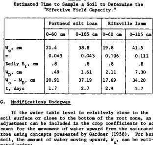
is the evapotranspiration for the day in

cm. The most representative time to sample a soil that has

been covered to prevent evaporation after a thorough

irri-gation can be obtained by integrating equation (17) between

the limits of Wo and WD.

t = (

14

cW

)

1

(19)

Since dW/dt rapidly + 0 using equation (17), about 5 to 20

days of calculations are needed before dW/dt < 0.01 cm

day I. Example calculations based on data from southern

Idaho and unpublished data from D.E. Miller (USDA-ARS-SWC,

Prosser, Washington) are summarized in Tab

j

e 2.

In these

examples, Et was assumed to be 0.8 cm day -i . In detailed

laboratory measurements, Miller and Aarstad (1971) found

that sampling 3.5 days after irrigation slightly

underesti-mated the available water for the 0- to 70-cm depth, and

TABLE 2

Estimated Time

to Sample a Soil to Determine the

"Effective Field Capacity."

Portneuf silt loam

Ritzvi le loam

0-60

cm

0-105 cm 0-60 cm

0-105 cm

Wo , cm

21.4

38.8

19.8

41.5

m

0.043

0.043

0.106

0.111

Daily E t , cm

.8

.8

.8

.8

WD , cm

.49

1.61

2.11

7.30

Wo - WD' cm

20.91

37.19

17.69

34.20

t, days

1.7

2.7

2.9

5.7

G. Modifications Underway

If the water table level is relatively close to the

soil surface or close to the bottom of

the root zone, an adjustment can be included in the crop coefficients to ac-count for the movement of water upward from the saturated zone using concepts presented by Gardner (1958). For bare soil, the amount of water moving upward, W

u

, can be esti-mated using:

W

u -

0.9

z i n

E

atl)

for z > a w — C

with a crop,

fAM - a4 ][ z e in

(

Wu m 1 100 - a4j zw - zr Et

where z is the effective height of the capillary fringe

above

tffe water

table, cm; zw is the depth to the water

ta-ble, cm; z r is the depth of roots, cm; AM is available soil

(20)

water to Z r in percent; a4

is

a constant (about 25); and is a constant for a given soil and crop (expected to vary between 1 and 3). An example of this approximation of W u is presented in Figure 1 using unpublished data from L.N. Namken (USDA-ARS-SWC, Weslaco, Texas). (Constants used in equation (20) are zw = 273 cm, z c = 50 cm, n = 1.22, and a

4 = 25%.)

q O.2 04 0.6 0.6 10 OBSERVED Wu ( cm day" 1 )

accuracy of all projected irrigations.

Summary

Irrigation programming practices have not changed ap-preciably in many areas during the past three decades be-cause suggested techniques have not been acceptable, and the direct and indirect

effects of excessive water use were

not readily apparent.

Several

alternative methods of pro-gramming irrigations are now available. The scheduling of irrigations for each field using meteorological, soil, and crop data, coupled with field inspection, appears to be an economical and acceptable irrigation management service in the U.S.A. An irrigation management service requires tech-nical competence and a good communications network. Relia-ble meteorological data also require technical competence,

and periodic calibration of instruments.

The USDA-ARS-SWC irrigation scheduling computer program using meteorological techniques and soil-crop data is de-scribed in this chapter. Since its development and use for

several years in Arizona,

Idaho, and Nebraska, several mod-ifications have been completed and others are under way.

This problem has enabled private firms and

service

agencies to gain experience in providing irrigation

management

ser-vice while

additional refinements are under way.

References

1. Baier, W. (1967). Recent advancements in the use of standard climatic data for estimating soil moisture.

Ann. Arid Zone 6, 1-21.

2. Beier, W. (1969). Concepts of soils moisture availa-bility and their effect on soil

moisture estimates from

a meteorological budget. Agr. Meteorol. 6, 165-178. 3. Bever, L.D. (1954). The meteorological approach to

ir-rigation control. Hawaiian Planter's Record 54, 291-298.

4. Brawn, R.J. and Buchheim, J.F. (1971). Water schedul-ing in southern Idaho, "A Progress Report," USDI Bur. of Reclamation. (Presented at the Nat. Conf. on Water Resources Eng., ASCE, Phoenix, Ariz., 1971.)

5. Budyko, I.I. (1956). The heat balance of the earth's surface. U.S. Dept. Com . Weather Bur. PB 131692

6. Corey, P.C. (1970). Irrigation scheduling by computer. Presented at the Joint Canv, of the Neb. State Irrig. Assn. and the Neb. Reclamation Assn., Grand Island, Neb., 1970.

7. Das, U.K. (1936). A suggested scheme of irrigation control using the day-degree system. Hawaiian Plan-ter's Record 37, 109-111.

8. Denmead, 0.T. and Shaw, R.H. (1959). Evapotranspira-tion in relaEvapotranspira-tion to the development of the corn crop. Agron J. 51, 725-726.

9. Fitzpatrick, E.A. and Cossens, G.G. (1966).

Applica-tions of Penman's and Thornthwaite's methods of

esti-mating transpiration rates to determination of moisture

of three Central Otago soils. N.Z. J. Agric. Res. 9, 985-994.

10. Fitzpatrick, B.A. and Stern, W.R. (1965). Components of the radiation balance of irrigated plots in a dry monsoonal environment. J. Applied Meteorol. 4, 649-660. 11. Franzoy, C.E. and Tankersley, E.L. (1970). Predicting

irrigations from climatic data and soil parameters. Trans. Amer. Soc. Agr. Engs. 13, 814-816.

12. Fritz, S. (1949). Solar radiation during cloudless days. Heating & Ventilating 46, 69-74.

13. Gardner, W.R. (1958). Some steady state solutions of the unsaturated moisture flow equation with application to evaporation from a water table. Soil Sci. 85, 228-232.

14. Goss, J.R. and Brooks, P.A. (1956). Constants for em-pirical expressions for downcoming atmospheric radia-tion under cloudless skies. J. Meteorol. 13, 482-488. 15. Heermann, D.F. and Jensen, M.E. (1970). Adapting

me-teorological approaches in irrigation scheduling. Proc. ASAE Nat. Irrig. Symp., Lincoln, Neb., 1970, 00-1 to 00-10.

16. Israelsen, 0.W., et al. (1944). Water application ef-ficiencies in irrigation. Utah Agr. Exp. Sta. Bul. 311. 17. Jensen, M.E. (1968). Water consumption by agricultural

plants. In "Water Deficits and Plant Growth" (T.T. Kozlowski, ed.), Vol. II, pp. 1-22. Academic Press, New York.

18. Jensen, M.E. (1969). Scheduling irrigations using com-puters. J. Soil and Water Conserv. 24, 193-195.

20. Jensen, M.E., Wright, J.L., and Pratt, B.J. (1971). Estimating soil moisture depletion from climate, crop, and soil data. Trans. Amer. Soc. Agr. Eng. Winter Meeting, 1969, Paper No. 69-641 (in press).

21. Jensen, M.E. and Heermann, D.P. (1970). Meteorological approaches to irrigation scheduling. Proc. Amer. Soc. Agr. Eng. Nat. Irrig. Symp., Lincoln, Neb, 1970, NN-1 to NN-10.

22. Makkink, G.F. and van Hermst, H.D.J. (1956). The ac-tual evapotranspiration as a function of the potential

evapo-transpiration

and the soil moisture tension.

Neth. J. Agr. Sci. 4.

23. Marshall, W.G. (1971). Operating a farm consulting

business. Proc. Sprinkler Irrig. Tech. Conf er Denver,

Colo 1971.

24. Miller, D.E. (1967). Available water in soil as influ-enced by extraction of soil water by plants. Agron. J. 59, 420-423.

25. Miller, D.E. and Aarstad, J.S. (1971). Available water as related to evapotranspiration rates and deep drain-age. Soil Sci. Soc. Amer. Proc. 35,.131-134.

26. Ogata, G. and Richards, L.A. (1957). Water content changes -following irrigation of bare-field soil that is protected from evaporation. Soil Sci. Soc. Amer. Proc. 21, 355-356.

27. Penman, H.L. (1948). Natural evaporation from open wa-ter, bare soil and grass. Proc. Roy. Soc. A93, 120-145. 28. Penman, H.L. (1952). The physical basis of irrigation

control. Proc. Int. Hort. Cong. t. London 13, 913-924. 29. Penman, H.L. (1963). Vegetation and hydrology. Tech.

Commun. No. 53, Commonwealth Bur. of Soils, Harpenden, England.

30. Pierce, L.T. (1958). Estimating seasonal and short-term fluctuations in

evapo-transpiration from meadow

crops. Bul. Amer. Meteor. Soc. 39, 73-78.

31. Pierce, L.T. (1960). A practical method of determining

evapotranspiration from temperature

and rainfall.

Amer. Soc. Agr. Eng. Trans. 3, 77-81.

32. Pruitt, W.O. and Jensen, M.C. (1955). Determining when

to irrigate. Agr. Eng. 36, 389-393.

33. Rickard, D.S. (1957). A comparison between measured

and calculated soil moisture deficit. N.Z. J. Sci. and

Tech. 38, 1081-1090.

T

OPTIMIZING THE SOIL ENVIRONMENT

subhumid climate: I. Micrometeorological influences. Agron. J. 63, 51-55.

35. Ritchie, J.T. and Burnett, E. (1971). Dryland evapora-tive flux in a subhumid climate: II. Plant influences. Agron. J. 63, 56-62.

36. Rosenberg, N.J. (1969). Seasonal patterns in evapo-transpiration by irrigated alfalfa in the Central Great Plains. Agron. J. 61, 879-889.

37. Thornthwaite, C.W. (1948). An approach toward a ra-tional classification of climate. Geograph. Rev. 38, 55-94.

38. Tyler, C.L., Corey, G.L., and Swarner, L.R. (1964). Evaluating water

use on a

new irrigation project. Ida-ho Agr. Exp. Sta. Res. Bul. No. 62.

39. van Bavel, C.H.M. (1960). Use of climatic data in guiding water management on the farm. In "Water and Agriculture," pp. 80-100. Amer. Assn. Advan. Sci. 40. van Bavel, C.H.M. (1966). Potential evaporation: The

combination concept and its experimental verification. Water Resources Res. 2, 455-467.

41. van Bavel, C.H.M. and Wilson, T.V. (1952). Evapotrans-piration estimates as a criteria for determining time of irrigation. Agr. Eng. 33, 417-418, 420.

42. van Wijk, W.A. and de Vries, D.A. (1954). Evapotrans-piration. Neth. J. Agr. Sci. 2, 105-119.

43. Wilcox, J.C. (1960). Rate of soil drainage following

irrigation. II. Effects on determination of rate of

consumptive use. Can. J. Soil Sci. 40, 15-27.

44. Willardson, L.S. (1967). "Irrigation Efficiency in the

Escalante Valley, Utah." Utah Resources Series 37,

Utah Agr. Exp. Sta.