Some Estimators for the Population Mean Using Auxiliary Information Under Ranked Set Sampling

Methods

Volume 8 | Issue 1

Article 24

5-1-2009

Some Estimators for the Population Mean Using

Auxiliary Information Under Ranked Set Sampling

Walid A. Abu-Dayyeh

Sultan Qaboos University, [email protected]

M. S. Ahmed

Sultan Qaboos University, [email protected]

R. A. Ahmed

Yarmouk University

Hassen A. Muttlak

King Fahd University of Petroleum & Minerals, [email protected]

Follow this and additional works at:

http://digitalcommons.wayne.edu/jmasm

Part of the

Applied Statistics Commons

,

Social and Behavioral Sciences Commons

, and the

Statistical Theory Commons

This Regular Article is brought to you for free and open access by the Open Access Journals at DigitalCommons@WayneState. It has been accepted for inclusion in Journal of Modern Applied Statistical Methods by an authorized administrator of DigitalCommons@WayneState.

Recommended Citation

Abu-Dayyeh, Walid A.; Ahmed, M. S.; Ahmed, R. A.; and Muttlak, Hassen A. (2009) "Some Estimators for the Population Mean Using Auxiliary Information Under Ranked Set Sampling,"Journal of Modern Applied Statistical Methods: Vol. 8: Iss. 1, Article 24. Available at:http://digitalcommons.wayne.edu/jmasm/vol8/iss1/24

253

Some Estimators for the Population Mean Using Auxiliary Information

Under Ranked Set Sampling

Walid A. Abu-Dayyeh

M .S. Ahmed

R. A. Ahmed

Sultan Qaboos University Sultan Qaboos University Yarmouk University

Hassen A. Muttlak

King Fahd University of Petroleum & Minerals

Auxiliary information is used along with ranking information to derive several classes of estimators to estimate the population mean of a variable of interest based on RSS (ranked set sample). The properties of these newly suggested estimators were examined. Comparisons between special cases of these estimators and other known estimators are made using a real data set. Some of the new estimators are superior to the old ones in terms of bias and mean square error.

Keywords: Auxiliary variables, efficiency, ranking, ranked set sample.

Introduction

Many authors have discussed the use of supplementary information of auxiliary variables in survey sampling to improve the existing estimators (for example, Cochran, 1977). The ratio estimator is among the most commonly adopted to estimate: (1) population means, or (2) the total of some variable of interest from a finite population with the help of an auxiliary variable when the correlation coefficient between the two variables is positive. When the correlation coefficient between the two variables is negative, the product estimator is used. These estimators are more efficient, i.e. have smaller

Walid Abu-Dayyeh is an associate Professor in the Department of Mathematics and Statistics at Suktan Qaboos University/Sultanate of Oman. Email: [email protected]. M .S. Ahmed is an Associate Professor in the Department of Mathematics and Statistics at Suktan Qaboos University, Sultanate of Oman. Email: [email protected]. R. A. Ahmed is a Lecturer at Almosul Unvirsity/Iraq. Hassen A. Muttlak is a Professor in the Department of Mathematics and Statistics at King Fahd University of Petroleum & Minerals, Saudi Arabia. Email: [email protected].

variances than the usual estimators of the population mean based on the sample mean of a simple random sample (SRS).

Ranked set sampling (RSS) can be used when the measurement of sample units drawn from a population of interest is very laborious or costly, but several elements can be easily arranged (ranked) in the order of magnitude. Takahasi and Wakimoto (1968) established the theory of RSS. They showed that the mean of the RSS is an unbiased estimator for the population mean and is more efficient than the mean of SRS. Dell and Clutter (1972) studied the effect of ranking error on the efficiency of RSS. The RSS has many statistical applications in biology and environmental studies (Barabesi & El-Sharaawi, 2001), for example, McIntyre (1952) first suggested using RSS to estimate the yield of pasture. In addition, RSS has been investigated by many researchers (Stokes, 1977; Stokes & Sager, 1988; Lam, et al., 1994, 1980; Mode, et al., 1999; Al-Saleh & Al-Shrafat, 2001; Al-Saleh & Zheng, 2000; Al-Saleh & Al-Omary, 2000), for more details about RSS, see Kaur, et al., 1995.

The RSS method can be summarized as follows: Select m random samples of size m units each and rank the units within each sample with respect to the variable of interest by a visual inspection or some other simple method.

254

Next, select for actual measurement the

i

th

smallest unit from the

i

thsample for i =1, 2,..., m. In this way, a total of m measured units are obtained, one from each sample. The cycle may be repeated r times to get a sample of size n = rm. These n = rm units form the RSS data. Note that in RSS,

rm

2 elements are identified, but

only rm _{of them are quantified. Thus,}

comparing this sample with a simple random sample (SRS) of size rm is reasonable.

Some Notions and Preliminaries

Let Y denote the variable of interest whose population mean and variance are

μ

_yand

2

y

σ

respectively. Estimate

μ

_y using the

information provided by one or two auxiliary variables

X

₁ and

X

₂based on SRS and RSS will be considered. Let

μ

_xiand 2

i

x

σ

be the

population mean and variance for

X

_i

,

i

=

1, 2

. Let

Y

_j

,

X

_1jand

X

_2jdenote the values of the variables

Y

,

X

₁and respectively, on the

th

j

unit of the population. The population means 1

x

μ

and

2

x

μ

of the auxiliary variables are

assumed to be known.

LetY_{( )i j}, X_{1( )i j}and X_{2( )i j}represent the

ith _{order statistics of a sample of size m in the j}th

cycle of the variables

Y X

,

₁and

X

₂ respectively based on a RSS of size n = rm drawn from the population. The sample mean for each variable using RSS data are defined as follows:

( )



( ) = =

=

r j m i i j n

Y

n

Y

1 1

1

, ( ) ( ) 1 1 1 1

1

,

r m n i j j i

X

X

n

_{= =}

=



and ( )



( ) = =

=

r j m i i j n

X

n

X

1 1 2 2

1

.

Consider the following notations:

( )i

(

( )i

)

y y y T =

μ

−

μ

, ( )

(

( )

)

1i 1i 1 x x x T =

μ

−

μ

, ( )

(

( )

)

2i 2i 2 x x x T =

μ

−

μ

, ( )

(

( )

)

(

( )

)

1i i 1 1 yx y y x i x T =

μ

−

μ

μ

−

μ

, ( )

(

( )

)

(

( )

)

2i i 2i 2 yx y y x x T =

μ

−

μ

μ

−

μ

, ( )

(

( )

)

(

( )

)

1 2i 1i 1 2i 2 x x x x x x T =

μ

−

μ

μ

−

μ

, ( )

(

( ) ( )

)

(

( ) ( )

)

1i 1 1 yx

E Y

i yi

X

i x i

σ

=

−

μ

−

μ

, ( )

(

( ) ( )

)

(

( ) ( )

)

2i 2 2 yx

E Y

i y i

X

i x i

σ

=

−

μ

−

μ

, ( )

(

( ) ( )

)

(

( ) ( )

)

1 2i 1 1 2 2 x x

E X

i x i

X

i x i

σ

=

−

μ

−

μ

. then: ( ) 1 0 i n y i T = =



, _{( )} 1 1 0 n x i i T = =



, _{2( )} 1 0 n x i i T = =



, ( ) ( ) 2 2 2 1 i 1 i n n y y y i i n T

σ

σ

= = = −





, ( ) ( ) 1 1 1 2 2 2 1 i 1 i n n x x x i i n T

σ

σ

= = = −





, ( ) ( ) 1 2 1 1 1 , n n yx yx yx i i i i n T

σ

σ

= = = −





( ) ( ) 2 2 2 1 1 n n yx yx yx i i i i n T

σ

σ

= = = −





( ) ( ) 1 2 1 2 1 2 1 i 1 i n n x x x x x x i i n T

σ

σ

= = = −





and ( ) ( ) 2 2 2 2 2 2 1 i 1 i n n x x x i i n T

σ

σ

= = = −





.

The following classes of estimators of the mean of the variable Y based on RSS are:

( ) ( ) ( ) 1 2 1 2 1 2 1 2 , a a n n a a n x x

X

X

Y

Y

μ

μ



 



=



_

 

_{ }



_



 



 _(2.1)

and

2

X

255

( ) ( ) ( ) 1 2 1 2 1 2 , 1 2 1 2 w w a a n n n x x Y X X Y w w

μ

μ

=  _{   }   _{  +  }       _{   }     (2.2)

where

a

₁

,

a

₂

,

w

₁,

w

₂ are constants and

1 2 1

w +w = .

Estimators Based on RSS and One or Two Auxiliary Variables

It is not possible to rank two or more dimensional data, therefore, ranking one of the variables and taking the corresponding values of other variables is an option. Assuming that the variable can be ranked perfectly - there are no errors in ranking the units, there will be errors in ranking the other variables.

Ranking on Study Variable Y

Assume that the ranking on variable

Y

is perfect while the ranking on variables

X

₁and

2

X

will have errors; the estimators (2.1) and (2.2) are respectively given by:

( ) [ ] [ ] 1 2 1 2 1 2 a a n n a n x x

X

X

Y

Y

μ

μ



 



=



_

 

_{ }



_



 



 _{, (3.1)} and ( ) [ ] ( ) [ ] 1 2 1 2 1 2 1 2 . w a a n n n n x x Y X X w Y w Y

μ

μ

=     +              (3.2) where [ ]



[ ] = =

=

r j m i i j n

X

n

X

1 1 1 1

1

and [ ]



[ ] = =

=

r j m i i j n

_n

X

X

1 1 2 2

1

are the sample means of the RSS for

X

₁and

2

X

respectively and

X

_{1[ ]i j}and

X

_{2[ ]i j} are the

th

i

judgment order statistic of the ith _{sample of}

the

j

thcycle, of the variables

X

₁ and

X

₂ respectively. Let ( ) y y n

Y

e

μ

μ

−

=

0 , [ ] 1 1 1 1 x x n

X

e

μ

μ

−

=

and [ ] 2 2 2 2 x x n

X

e

μ

μ

−

=

.

Obtain the bias and the MSE of the estimators

Y

~

_aand

Y

~

_wrespectively up to the order of

n

−1as follows:

( )

[ ] [ ]

(

)

[ ]

(

)

[ ] [ ] 1 1 2 2 1 2 1 1 2 2 2 2 1 2 1 2 1 2 1 2 2 2 1 1 1 1 2 2 2 2 1 2 2 2 2 2 2 1 1 2 2 1 ( ) ( ) 1 ( ) 2 1 ( ) 2 ( ) i i i i i a m m yx yx yx yx i i x x m y x x i x m y x x i x m y x x x x i x x B Y a a m T m T rm rm a a m T rm a a m T rm a a m T rm

σ

σ

μ

μ

μ

σ

μ

μ

σ

μ

μ

σ

μ μ

= = = = = = − + − − + − + − − + −











 (3.3) The MSE of

Y

~

_a when ranking on variable Y is:

( )

( ) [ ] [ ] [ ] [ ] [ ] 1 1 1 2 2 1 1 2 1 2 2 1 2 1 2 2 1 2 2 2 2 2 2 2 1 1 1 2 2 2 2 2 2 2 2 2 1 1 1 2 2 2 2 2 2 1 2 1 1 2 2 ( ) ( ) 2 ( ) 2 ( ) 2 ( ) i i i i i i a m m y y y x x i i x m m y x x y yx yx i i x y x m m y yx yx y x x x x i i y x x x MSE Y m T a m T rm rm a m T a m T rm rm a m T a a m T rm rm σ μ σ μ μ σ μ σ μ μ μ μ σ μ σ μ μ μ μ = = = = = = = − − + + − − + − − + +













 (3.4)

256

up to the order of _n−1_{. The optimum values of} 1

a

and

a

₂, which minimize the MSE of

Y

~

_a, are obtained by the derivation of (3.4) with respect to

a

₁and

a

₂ respectively [ ] [ ] [ ] [ ] [ ] [ ] [ ] 1 1 1 2 2 2 2 1 2 1 2 1 1 2 2 1 2 1 2 1 2 2 1 1 1 1 2 2 2 2 1 1 1

(

)(

)

(

)(

)

(

)(

)

(

)

i i i i i i i m m x yx yx x x i i m m yx yx x x x x i i m m y x x x x i i m x x x x i

a

m

T

m

T

m

T

m

T

m

T

m

T

m

T

μ

σ

σ

σ

σ

μ

σ

σ

σ

∗ = = = = = = =

=

−

−

−

−

−

−

−

−

−

−















(3.5) [ ] [ ] [ ] [ ] [ ] [ ] [ ] 2 2 2 1 1 1 1 1 2 1 2 1 1 2 2 1 2 1 2 2 2 2 1 1 1 1 2 2 2 2 1 1 1 ( )( ) ( )( ) ( )( ) ( ) i i i i i i i m m x yx yx x x i i m m yx yx x x x x i i m m m y x x x x x x x x i i i a m T m T m T m T m T m T m T μ σ σ σ σ μ σ σ σ ∗ = = = = = = = = − − − − − − − − − −















(3.6) The minimum MSE up to terms of

n

−1 for the class

Y

~

_a∗ is:

( )

[ ] [ ] ( ) [ ] 1 1 2 2 2 2 1 1 1 1 2 2 1 2 1 2 1 1 2 2 min 2 2 2 2 1 1 2 2 2 2 2 1 1 ₁ 2 2 2 2 1 1 1 2 2 2 2 1 1 1 [( ) ( ) ( ) ( ) ( ) 2 ( )( )( ) ( )( ) ( i i i i a m m yx yx x x i i m m m yx yx x x y y i i _i m m m x x x x x x x x i i i m m x x x x i i MSE Y m T m T rm m T m T m T m T m T m T m T m T m σ σ σ σ σ σ σ σ σ σ σ ∗ = = = = ₌ = = = = = = − − + − − − − − − − − − − −



 [ ] 1 2 1 2 2 1 ] ) i m x x x x i=T − (3.7)

If

a

₁and

a

₂take the values in (3.5) and (3.6) respectively, the bias of

Y

~

_afrom (3.3) is given by:

( )

[ ] [ ] [ ] 1 1 2 2 1 2 1 2 min 1 2 2 2 2 2 2 1 1 2 1 {[ ][ ] [ ] } i i i a m m y x x x x i i m x x x x i B Y g rm m T m T m T

μ

σ

σ

σ

∗ = = = = − − − −







 (3.8) where

g

₁ is given in the Appendix.

The bias and the MSE of the estimators of (3.2) are given by:

( )

[ ] [ ]

(

)

[ ]

(

)

[ ] 1 1 1 2 2 2 1 1 2 2 2 2 1 1 2 1 2 2 2 1 1 1 1 2 2 2 2 1 2 2 2 2 2 2 2 1

{

[

]

[

]

1

[

]

2

1

[

]},

2

μ

σ

μ μ

σ

μ μ

σ

μ

σ

μ

= = = =

=

−

+

−

−

+

−

−

+

−









 i i i i m w y yx yx i y x m yx yx i y x m x x i x m x x i x

a w

B Y

m

T

rm

a w

m

T

rm

w a a

m

T

rm

w a a

m

T

rm

(3.9) up to the order of

n

−1. The MSE of the estimator Y_wif ranking on variable

Y

is:

257

( )

( ) [ ] [ ] [ ] [ ] [ ] 1 1 1 2 2 1 1 2 1 2 2 1 2 1 2 2 1 2 2 2 2 2 2 2 1 1 2 1 1 2 2 2 2 2 2 2 2 2 2 1 1 1 1 2 2 2 2 2 1 2 1 2 1 1 2 2 [ ] { [ ] 2 [ ] 2 [ ] 2 [ ] }

σ

σ

μ

μ

μ

σ

σ

μ

μ μ

σ

σ

μ μ

μ μ

= = = = = = − − = + + − − + + − − +













 i i i i i i m m y y x x i i w y y x m m x x yx yx i i x y x m m yx yx x x x x i i y x x x m T w a m T MSE Y rm rm w a m T wa m T rm rm w a m T ww a a m T rm rm (3.10) if

a

₁and

a

₂are both known and take the values in (3.5) and (3.6) respectively, up to order

n

−1.

The optimum values of

w

₁ and

w

₂, which minimize the MSE of

Y

~

_w, obtained by the derivation of equation (3.10) with respect to

w

₁ under the restrictionw₁+w₂ =1, are given by:

[ ] [ ] [ ] [ ] [ ] [ ] [ ] 2 2 1 1 2 2 1 2 1 2 1 1 2 2 1 2 1 2 1 2 2 2 2 1 1 1 2 1 2 1 1 2 2 2 2 2 2 1 2 1 1 1 2 1 2 i i i i i i i m m x x yx yx i i m m yx yx x x x x i i m m x x x x i i m x x x x i w a m T a m T a m T a a m T a m T a m T a a m T

σ

σ

σ

σ

σ

σ

σ

∗ = = = = = = = =     − − − +             − − −             − + − −           −    















and the MSE of

( ) [ ] ( ) [ ] 1 2 1 2 1 2 1 2 a a n n n n w x x

X

X

Y

w Y

w Y

μ

μ

∗ ∗ ∗

















=

_

_

+

_

_











(3.12)

is the minimum MSE up to terms of _n−1_{. As for} the class

Y

~

_w:

( )

( ) [ ] [ ] _{[ ]} [ ] _{[ ]} 1 1 2 2 1 2 1 2 2 2 1 1 2 min 2 2 2 2 2 2 1 1 2 1 1 2 2 2 1 2 1 1 2 2 2 1 2 1 1 1 2 1 2 2 i i i _i i _i w m m y y x x i i m m x x x x x x i i m m x x yx yx i i yx MSE Y m T w a m T rm a m T a a m T w a m T a m T a m

σ

σ

σ

σ

σ

σ

σ

∗ ∗ = = = = ∗ = = =       _{− + −}    _              +  − −  − _          −  _{ } − −  −      +













 [ ] [ ] [ ] [ ] 2 1 2 1 2 2 2 2 2 1 2 1 1 2 2 2 2 2 2 2 1 1 2 i i i i m m yx x x x x i i m m x x x x i i T a a m T a m T a m T

σ

σ

σ

= = = =      − − −     _         _ +  −  +  −      









(3.13) If

w

takes the value in (3.11), then bias of

Y

~

_w

from (3.9) is given by:

( )

[ ] [ ]

(

)

[ ]

(

)

[ ]

(

)

[ ] [ ] 1 1 2 2 1 1 2 2 2 2 2 2 1 1 2 1 1 2 2 2 2 1 1 2 2 1 1 2 2 2 2 2 1 1 1 1 2 2 1 2 i i i i i i w m m y yx yx yx yx i i m m x x x x i i m m x x yx yx i i B Y w a m T a m T a a a a m T m T a a m T a m T μ σ σ σ σ σ σ ∗ ∗ = = = = = = =        − − −               −   −   + +_ − _− _ −    −     + + − +  −     













 (3.14) Ranking on One Auxiliary Variable

If the ranking of

X

₁ is perfect, then the two estimators (2.1) and (2.2) are given by:

[ ] ( ) [ ] 1 2 1 2 1 2 a a n n a n x x

X

X

Y

Y

μ

μ



 





 



=

_

_{ }

_



 





_(3.15) and

258

[ ] ( ) ( ) [ ] 1 2 1 2 1 2 1 2 a a n n w n n x x

X

X

Y

w Y

w Y

μ

μ

















=

_

_

+

_

_











(3.16) The formulas for the bias and MSE of estimators (3.15) and (3.16) respectively will be the same as in 3.1 except for the current estimators replace

[ ]

by

( )

in

X

₁, and

( )

by

[ ]

in

Y

.

Similarly if the ranking on

X

₂ is perfect, then the estimators:

[ ] ( ) [ ] 1 2 1 2 1 2 a a n n a n x x

X

X

Y

Y

μ

μ



 





 



=

_

_{ }

_



 





_(3.17) [ ] ( ) ( ) [ ] 1 2 1 2 1 2 1 2 a a n n w n n x x

X

X

Y

w Y

w Y

μ

μ

















=

_

_

+

_

_











_(3.18) result.

The formulas for the bias and the MSE

of estimators (3.17) and (3.18) respectively, will be the same as in 3.1 except for the case of replacing

[ ]

by

( )

in

X

₂, and

( )

by

[ ]

in

Y

(

a

₁

₌

0

or

a

₂

₌

0

in (2.1) and

w

₁

₌

0

or

2

0

w

₌

correspond to the case of one auxiliary variable).

Comparisons of Estimators

Consider the following known estimators. The RSS sample mean of the data:

( )



( ) = =

=

r j m i i j n

Y

n

Y

1 1

1

is an unbiased estimator for the population mean and its variance is given by:

( )

( )

( ) 2 2 2 1

1

[

]

i m y y n i

Var Y

m

T

rm

σ

₌

=

−



(Takahasi & Wakimoto, 1968).

The Ratio estimator using RSS data is defined as: ( ) [ ]n x n R

X

Y

Y

₌

μ

.

This estimator is a special case of the estimator in equation (1) where

a

₁

_{= −}

1

and a

₁

₌

0

. The

bias and the

MSE

of this estimator are

respectively given by:

( )

[ ] [ ] 1 2 2 2 1

1

i i R m yx yx i y m x x x i x

B Y

m

T

rm

m

T

σ

μ

μ

_σ

μ

= =

=









−

−



















_

_



−



_

_



















( )

( ) [ ] [ ] 2 2 2 2 2 2 2 1 1 2 1

1

1

2

i i i R m m y y x x i i y x y m yx yx i y x

MSE Y

m

T

m

T

rm

m

T

σ

σ

μ

μ

μ

σ

μ μ

= = =

=













−

+

−

−



























_

_





_

₋

_





_

_













(Samawi & Muttlak, 1996).

The product estimator using RSS data is defined as: ( ) [ ] x n n P

X

Y

Y

μ

=

This estimator is a special case for the estimator in equation (1) where

a

₁

₌

1

and a

₁

₌

0

. The new estimator is called the product estimator and its bias and

MSE

respectively are given by

( )

2 _{[ ]} 1

[

]

i m y P yx yx i

B Y

m

T

rm

μ

σ

=

=

−



259

( )

_{( )} [ ] [ ] 2 2 2 2 2 1 2 2 2 1 1

1

{

[

]

1

2

[

]

[

]}

μ

σ

μ

σ

σ

μ μ

μ

= = =

=

−

+

−

+

−







i i i m y P y y i y m m x x yx yx i y x i x

MSE Y

m

T

rm

m

T

m

T

If

a

₁

=

a

₂

=

−

1

is set in the estimator of equation (2) the following new estimator results:

( ) [ ] [ ] 1 2 1 2

.

x x a n n n

Y

Y

X

X

μ

μ

=



The bias and the

MSE

are respectively given by

( )

_{[ ]} [ ] [ ] [ ] [ ]

}

1 1 1 2 2 1 2 1 2 1 2 2 1 1 2 2 1 2 2 2 2 2 1 2 2 2 1 1 1 1 1 1 1 1 1

μ

σ

μ

σ

σ

μ μ

μ

σ

σ

μ μ

μ μ

= = = = = = − + − + − − − − −

 



 

_



_





























































 i i i i i m y a x x i x m m x x x x x x i x x i x m m yx yx yx yx i i y x y x B Y m T rm m T m T m T m T and

( )

_{( )} [ ] [ ] [ ] [ ] [ ] 1 1 2 2 1 2 1 1 2 2 1 2 1 2 1 2 1 2 2 2 2 2 2 1 2 2 2 2 2 2 1 1 1 1 1 1 1 1 2 2 2 μ σ μ σ σ μ μ σ σ μ μ μ μ σ μ μ = = = = = = = − + − + − − − − − + −     _ _                                 













 i i i i i i m y a y y i y m m x x x x i i x x m m yx yx yx yx i i y x y x m x x x x i x x MSE Y m T rm m T m T m T m T m T

Setting

a

₁

=

a

₂

=

1

in the estimator of equation (2) results in a new estimator defined as: ( ) [ ] [ ] 2 1 2 1 x n x n n a

X

X

Y

Y

μ

μ

=





_.

The bias and the

MSE

are respectfully given by

( )

[ ] [ ] [ ] 1 2 1 2 1 2 1 1 2 2 1 2 2 1 1 1

1

1

1

μ

σ

μ μ

σ

σ

μ μ

μ μ

= = =

=



_

_



₋

₊



_

_

















−

+

−



























i i i a m y x x x x i x x m m yx yx yx yx i i y x y x

B Y

m

T

rm

m

T

m

T

and

( )

( ) 1 1 1 2 2 1 1 1 2 2 2 1 2 1 2 2 1 2 2 2 2 2 2 2 2 2 1 1 2 2 2 1 1 1 1 1 1 2 2 2 μ _{σ σ} μ μ σ _{μ μ} σ μ σ σ μ μ μ μ                     = = = = = =  _{   }                              = − + − + − + − + − + −











 i i i i i i a m m y y y x x i i y x m m x x yx yx i y x i x m yx yx x x x x i i y x x x MSE Y m T m T rm m T m T m T m T 1        



 m

If a₁ =a₂ =1 in the estimator of equation 3 is set, a new estimator called the Multivariate ratio estimator using RSS can be defined as

( ) [ ] [ ]









+









=

2 1 2 2 1 1 x n x n n w

X

w

X

w

Y

Y

μ

μ



.

The bias and the

MSE

are respectively given by

( )

_{[ ]} [ ] 1 1 1 2 2 2 1 1 2 1 i i m w y yx yx i y x m yx yx i y x

w

B Y

m

T

w

m

T

μ

σ

μ μ

σ

μ μ

= =



_

_



=



_

−

_

+













−

















260

and

( )

( ) [ ] [ ] [ ] [ ] [ ] 1 1 2 2 1 2 1 2 1 2 2 2 1 2 2 1 1 1 2 2 2 2 2 1 2 2 2 2 2 1 2 2 1 1 2 2 1 2 1 1 1

1

1

1

2

1

2

1

μ

_σ

μ

σ

σ

μ

μ

σ

σ

μ μ

μ

σ

μ μ

= = = = = =

 





=

_{ }

−

_









_

_

_

_



+

_

_

−

_

+

_

−

_

























−



−





−

_



−









_







−

−

















i i i i i i m y w y y i y m m x x x x i i x x m m x x x x x x i i x x x m yx yx i y x

MSE Y

m

T

rm

w

m

T

m

T

m

T

w

m

T

m

T

[ ] [ ] [ ] [ ] 2 2 2 1 2 1 2 1 2 2 2 2 2 2 2 1 1 2 2 2 1 1

1

1

1

2

.

σ

μ μ

σ

μ μ

σ

σ

μ μ

μ

= = = =







+

−





















−



−



















−

+

−



























i i i i m yx yx i y x m x x x x i x x m m x x yx yx i y x i x

m

T

m

T

m

T

m

T

The comparison between the estimators proposed is illustrated by using a real data set. The data for the illustration was taken from Ahmed (1995); the population consists of 332 villages. Consider the variables,

Y

,

X

₁and

X

₂ where

Y

is number of cultivators,

X

₁ is the area of the village and

X

₂ is the number of household in the village.

The following steps summarize the simulation procedure to find the bias and

MSE

of an estimator for the population mean using perfect ranking on the variable of interest Y. Step 1:

Simulate

rm

2observations from the 332 real data values with replacement and perform the RSS procedure with m =5 and r = 16 to get sample of size

n

=

rm

=

80

.

Step 2:

Use the data in Step 1 to calculate



_{( )}



_{( : )} 16 5



_{( : )} 1 1 1 1

1

1

80

r m n i m j i m j j i j i

Y

Y

Y

mr

_{= = = =}

=

 

=

 

where

Y



( : )i m jis the

i

th smallest in the sample of

size m =5 in the

_j

th_cycle.

Step 3:

Repeat steps 1 and 2 (30,000) times, using these 30,000 values to obtain

_{( )} 30000_{( )} 1 1 30000 n n i i Y Y = =



Step 4:

Find the approximate bias and MSE for ( )n

Y

ˆ

. The bias is obtained by

( )

( )

( ) 30000 1 1 ˆ ˆ 30000 y n n i i B Y Y

_μ

= =



− , and the

MSE

of

Y

ˆ

_{( )n} is obtained as

( )

( )

(

( ) ( )

)

2 30000 1

ˆ

ˆ

30000

1

ˆ

_

−

−

=

i ni n n

Y

Y

Y

MSE

.

The above simulation was preformed for all other estimators suggested ranking on one of the variables Y,

X

₁ or

X

₂. Calculate the efficiency of these estimators with respect to the



( )

( )n

(

( )n

)

MSE Y

₌

Var Y

estimator using



( )

( )

_{( )}

( )

,

ˆ

=

MSE Y

n

e Y

MSE Y

where

Y



represents any of the estimators given.

In Tables 1-3,

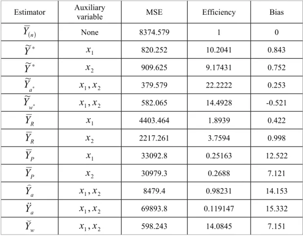
MSE

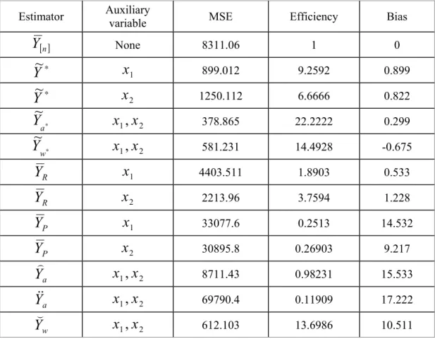
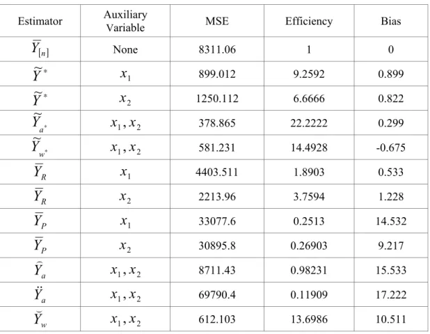
, bias, and

efficiency have been calculated for each of the suggested estimators. In Table 1, ranking on the variable Y is shown (i.e., the ranking of variable Y will be perfect while the ranking of the other variables will be with errors in ranking). Tables 2 and 3 show the ranking on the variables

X

₁ and

X

₂respectively.

Considering the results of Tables 1-3 it is observed that

Y

~

_a∗ dominates all other estimators and achieved the highest efficiency. Its efficiency is more than 22 times higher than the

261

Table 1: The Bias,

MSE

and the Efficiency for all Estimators Based on Ranking of the Variable

Y

Estimator Auxiliary

variable MSE Efficiency Bias

( )n

Y

None 8374.579 1 0 ∗

Y

~

x

1 820.252 10.2041 0.843 ∗

Y

~

x

2 909.625 9.17431 0.752 ∗ a

Y

~

x

1

,

x

2 379.579 22.2222 0.253 ∗ w

Y

~

x

1

,

x

2 582.065 14.4928 -0.521 R

Y

x

1 4403.464 1.8939 0.422 R

Y

x

2 2217.261 3.7594 0.998 P

Y

x

1 33092.8 0.25163 12.522 P

Y

x

2 30979.3 0.2688 7.121 a

Y



x

1

,

x

2 8479.4 0.98231 14.153 a

Y





x

1

,

x

2 69893.8 0.119147 15.332 w

Y



x

1

,

x

2 598.243 14.0845 7.151

262

Table 2: The Bias,

MSE

and the Efficiency for all Estimators Based on Ranking of the Variable

X

₁

Estimator Auxiliary _variable MSE Efficiency Bias

[ ]n

Y

None 8311.06 1 0 ∗

Y

~

x

1 899.012 9.2592 0.899 ∗

Y

~

x

2 1250.112 6.6666 0.822 ∗ a

Y

~

x

₁

,

x

₂ 378.865 22.2222 0.299 ∗ w

Y

~

x

₁

,

x

₂ 581.231 14.4928 -0.675 R

Y

x

1 4403.511 1.8903 0.533 R

Y

x

2 2213.96 3.7594 1.228 P

Y

33077.6 0.2513 14.532 P

Y

x

2 30895.8 0.26903 9.217 a

Y



x

1

,

x

2 8711.43 0.98231 15.533 a

Y





x

1

,

x

2 69790.4 0.11909 17.222 w

Y



x

1

,

x

2 612.103 13.6986 10.511 1

x

263

RSS estimator. Some other estimators achieved higher efficiency than

Y



( )n , theses estimators

are:

Y

~

_w∗,

Y



_w,

Y

~

∗, and

Y

_R.

The estimators achieved about the same efficiency no matter which variable was ranked on. This provides greater flexibility in choosing the variable to rank on, since some of the variables are more difficult to rank than others.

References

Ahmed, M. S. (1995) Some Estimation Procedure Using Multivariate Auxiliary Information in Sample Surveys (Ph. D. Thesis, Department of Statistics & Operations Research, Aligarh Muslim University, India).

Al-Saleh, M. Fraiwan & Al-Sharfat, K. (2001). Estimation of average milk yield using ranked set sampling. Environmetrics, 12, 395-399.

Al-Saleh, M. Fraiwan & Al-Omari,

Amer. (2002). Multi-Stage RSS. Journal of

Statistical Planning and Inference, 102, 273-286.

Al-Saleh, M. Fraiwan and Zheng, Gang. (2002). Estimation of Bivariate Characteristics Using Ranked Set Sampling. The Australian & New Zealand Journal of Statistics, 44, 221-232.

Barabesi, L. and El-Sharaawi A. (2001). The efficiency of ranked set sampling for parameter estimation. Statistics and Probability Letters, 53, 189-199.

Cochran, W. G. (1977) Sampling

techniques, 3rd edition (John Wily, NY). Table 3: The Bias,

MSE

and the Efficiency for all Estimators Based on Ranking of the

Variable

X

₁

Estimator Auxiliary

Variable MSE Efficiency Bias

[ ]n

Y

None 8311.06 1 0 ∗

Y

~

x

1 899.012 9.2592 0.899 ∗

Y

~

x

2 1250.112 6.6666 0.822 ∗ a

Y

~

x

1

,

x

2 378.865 22.2222 0.299 ∗ w

Y

~

x

1

,

x

2 581.231 14.4928 -0.675 R

Y

x

1 4403.511 1.8903 0.533 R

Y

x

2 2213.96 3.7594 1.228 P

Y

33077.6 0.2513 14.532 P

Y

x

2 30895.8 0.26903 9.217 a

Y



x

1

,

x

2 8711.43 0.98231 15.533 a

Y





x

1

,

x

2 69790.4 0.11909 17.222 w

Y



x

1

,

x

2 612.103 13.6986 10.511 1

x

264

Dell, D. R. and Clutter, J. L. (1972) Ranked set sampling theory with order statistics background, Biometrics, 28, 545-55.

Kaur, A., Patil, G. P., Sinha, B. K. and Taillie, C. (1995) Ranked set sampling: an

annotated bibliography, Environmental and

Ecological Statistics, 2, 25-54.

Lam, K., Sinha, B.K. and Wu, Z.(1994). Estimation of parameters in two-parameter Exponential distribution using ranked set sampling, Annals of the Institute of Statistical Mathematics, 46(4), 723-736.

McIntyre, G. A. (1952) A method of unbiased selective sampling, using ranked sets,

Australian Journal of Agricultural Research, 3, 385-390.

Mode, N., Conquest, L. & Marker, D. (1999). Ranked set sampling for ecological research: Accounting for the total cost of sampling. Environmetrics, 10, 179-194.

Samawi, H. M. & Muttlak, H. A. (1996) Estimation of ratio using rank set sampling,

Biometrical Journal, 38, 753-764.

Stokes, S. L. & Sager, T.(1988). Characterization of ranked set sample with application to estimating distribution functions.

Journal of the American Statistical Association,

83, 374-381.

Stokes, S. L. (1977): Ranked set sampling with concomitant variables,

Communications in statistics, A6, 1207-1211. Takahasi K. & Wakimoto K. (1968) On unbiased estimates of the population mean based on the sample stratified by means of ordering,

Annals of the Institute of Statistical Mathematics, 21, 249-55.

265

Appendix [ ] [ ] [ ] [ ] [ ] [ ] _{[ ] [ ]} 1 2 1 2 1 1 2 2 1 1 2 2 1 1 2 2 1 2 1 2 1 2 2 2 2 1 1 1 1 1 1 2 1 1 1

2

2

σ

σ

σ

σ

σ

σ

σ

σ

σ

= = = = = = = = =

−

−

−

−

−

−

−

−

−

−

−





 













_

_{ }

_

_

_

_

_



 





















































i i i i i i i m m m m m x x x x yx yx yx yx x x x x i i i i i m m m yx yx i yx yx x x x x yx i i i

g

m

T

m

T

m

T

m

T

m

T

m

T

m

T

m

T

m

[ ] [ ] [ ] [ ] [ ] [ ] [ ] [ ] [ ] 1 1 1 2 2 1 2 1 2 2 2 1 1 1 2 1 2 1 1 2 2 2 2 1 1 2 2 2 2 2 1 1 1 1 1 2 2 2 2 2 1 1

σ

σ

σ

σ

σ

σ

σ

σ

= = = = = = = = =

−

−

−

+

−

−

−

+

−

−























 

 









 

 









 

 







 





 





 





















i i i i i i i m m yx x x i i i m m m m m x x x x x x yx yx x x i x x x x i i i i i m m x x x x i i

T

m

T

m

T

m

T

m

T

m

T

m

T

m

T

m

T

[ ] [ ] [ ] [ ] [ ] [ ] [ ] [ ] [ ] 2 2 1 1 2 2 1 2 1 2 2 2 1 1 2 2 1 2 1 2 1 1 2 2 1 1 1 2 2 2 2 2 1 1 1 1 1 1

σ

σ

σ

σ

σ

σ

σ

σ

σ

= = = = = = = = =

−

+

−

−

−

−

−

−

−

−

+

−



 







 







 

































































i i i i i i i i m m m yx yx x x yx yx i i i m m m m m x x x x yx yx i x x x x x x x x i i i i i m yx yx i

m

T

m

T

m

T

m

T

m

T

m

T

m

T

m

T

m

T

_{[ ]} [ ] [ ] [ ] [ ] _{[ ] [ ] [ ]} 2 2 1 2 1 2 2 2 1 1 1 1 1 1 2 2 1 2 1 2 1 2 2 2 2 2 2 2 2 1 1 1 1 2 2 2 1 1 1 1

σ

σ

σ

σ

σ

σ

σ

σ

σ

= = = = = = = =

−

−

+

−

−

−

+

−

−

−

−



 



 

 





 



 

 





 



 

 







 







_



 





_{ }



 





_{ }

















i i i i i i m m m m x x i x x x x x x x x i i i i m m m m yx yx i yx yx x x x x x x x i i i i

m

T

m

T

m

T

m

T

m

T

m

T

m

T

m

T

m

[ ] [ ] [ ] _{[ ]} [ ] [ ] [ ] [ ] [ ] 1 2 2 2 2 1 1 1 1 2 2 2 2 1 1 1 1 2 2 1 2 2 2 2 2 2 2 2 1 1 1 1 1 2 2 2 2 1 1 1

σ

σ

σ

σ

σ

σ

σ

σ

= = = = = = = = =

−

−

−

−

+

−

−

+

−

−

−

















 















 













 





















































i i i _i i i i i m x i m m m m m x x x x yx yx x x yx yx i i i i i m m m x x x x i yx yx i i i

T

m

T

m

T

m

T

m

T

m

T

m

T

m

T

m

T

[ ] _{[ ]} [ ] 2 2 1 1 2 2 2 2 2 2 1 1 1

σ

σ

σ

= = =

+

−

−

−







 

_



_



_



























i _i i m m x x x x i i m yx yx i

m

T

m

T

m

T