Supplement to "Quantile-Based Nonparametric Inference for First-Price Auctions"

(1)

Supplement to “Quantile-Based Nonparametric

Inference for First-Price Auctions”

Vadim Marmer

University of British Columbia

Artyom Shneyerov

CIRANO, CIREQ, and Concordia University

August 30, 2010

Abstract

This paper contains supplemental materials for Marmer and Shneyerov (2010). We discuss here how the approach developed in the aforementioned paper can be applied to conducting inference on the optimal reserve price in first-price auctions, report additional simulations results, and provide a detailed proof of the bootstrap result in Marmer and Shneyerov (2010).

S.1 Introduction

This paper contains supplemental materials for Marmer and Shneyerov (2010), MS hereafter. Section S.2 discusses how the approach developed in MS can be applied to conducting inference on the optimal reserve price in first-price auctions. Section S.3 contains the full set of the Monte Carlo simulations results of which only a summary was reported in MS. In Section S.4, we provide a detailed proof of bootstrap Theorem 3 in MS.

(2)

S.2 Inference on the optimal reserve price

In this section, we consider a problem of conducting inference on the optimal reserve price. Several previous articles have studied that problem. Paarsch (1997) develops a parametric approach and applies his estimator to timber auctions in British Columbia. Haile and Tamer (2003) consider the problem of inference in an incomplete model of English auction, derive nonparametric bounds on the reserve price and apply them to the reserve price policy in the US Forest Service auctions. Closer to the subject of our paper, Li, Perrigne, and Vuong (2003) develop a semiparametric method to estimate the optimal reserve price. At a simplified level, their method essentially amounts to re-formulating the problem as a maximum estimator of the seller’s expected profit. Strong consistency of the estimator is shown, but its asymptotic distribution is as yet unknown.

We follow Haile and Tamer (2003) and make the following mild technical assump-tion on the distribuassump-tion of valuaassump-tions.1

Assumption S.1 Letcbe the seller’s own valuation. The function(p−c) (1−F (p|x)) is x-a.e. strictly pseudo-concave in p on (v(x),v¯(x)).

Let r∗(x) denote the optimal reserve price given the covariates value x. Under Assumption S.1 (see the discussion in Haile and Tamer (2003)), r∗(x) is found as the unique solution to the optimal monopoly pricing problem, and is given by the unique solution to the corresponding first-order condition:

r∗(x)− 1−F (r

∗₍_x₎_|_x₎

f(r∗₍_x₎_|_x₎ −c= 0. (S.1)

Remark. Even in the presence of a binding reserve price r(x) in the data, the optimal reserve price r∗(x) is still identifiable provided r∗(x) > r(x), for the ratio in (S.1) remains the same if we use the truncated distribution F∗(r∗(x)|x) defined in Section 5, and the associated density f∗(r∗(x)|x), in place of F(r∗(x)|x) and

f(r∗(x)|x). See the discussion of this in Haile and Tamer (2003).

One approach to the inference on r∗(x) is to estimate it as a solution ˆr∗(x) to (S.1) using consistent estimators forf andF in place of the true unknown functions.

1_{This condition is implied by the standard monotone virtual valuation condition of Myerson}

(3)

However, a difficulty arises because, even though our estimator ˆf(v|x) is asymptot-ically normal, it is not guaranteed to be a continuous function of v. We instead take a direct approach and construct confidens sets (CSs) that do not require a point estimate of r∗(x).

As discussed in Chapter 3.5 of Lehmann and Romano (2005), a natural CS for a parameter can be obtained by inverting a test of a series of simple hypotheses concerning the value of that parameter.2 We construct CSs for the optimal reserve price by inverting the test of the null hypothesesH0(v) :r∗(x) =v. Such hypotheses can be tested by testing the optimal reserve price restriction (S.1) atr∗(x) =v. Thus, the CSs are formed by collecting all valuesv for which the test fails to rejects the null that (S.1) holds atr∗(x) =v.

Consider H0(v) :r∗(x) = v, and the following test statistic:

where ˆF is defined in (17) in MS, and ˆVf(v, x) is a consistent plug-in estimator of the

asymptotic variance of ˆf(v|x), see MS Theorem 2. By MS Theorem 2 and Lemma 1(h), T (r∗(x)|x) →d N(0,1). Furthermore, due to uniqueness of the solution to

(S.1), for anyt >0,P(|T (v|x)|> t|r∗(x)6=v)→1. A CS forr∗ with the asymptotic coverage probability 1−α is formed by collecting all v’s such that a test based on

T (v|x) fails to reject the null at the significance levelα:

CS1−α(x) =

n

v ∈Λ (ˆ x) :|T(v|x)| ≤z1−α/2

o

,

where zτ is the τ quantile of the standard normal distribution. Asymptotically

CS1−α(x) has a correct coverage probability since by construction we have that

P (r∗(x)∈CS1−α(x)) = P |T(r∗(x)|x)| ≤z1−α/2

→1−α, provided that r∗(x)∈ Λ (x) = [Q(τ1|x), Q(τ2|x)].

When the seller’s own evaluation c is unknown, one can treat a CS as a function

2_{CSs obtained by test inversion have been used in the econometrics literature, for example, in}

the context of instrumental variable regression with weak instruments (Andrews and Stock, 2005), for constructing CSs for the date of a structural break (Elliott and M¨uller, 2007), and in the case of set identified models (Chernozhukov, Hong, and Tamer, 2007); see also the references on page 1268 of Chernozhukov, Hong, and Tamer (2007).

(4)

of cand, using the above approach, construct conditional CSs for chosen values of c.

S.3 Monte Carlo results

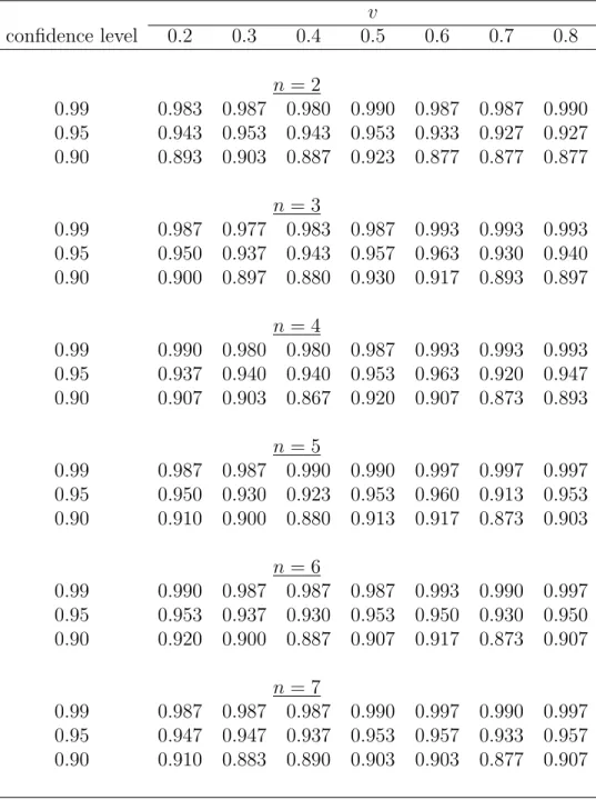
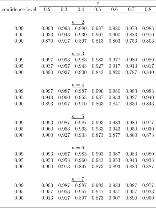
In this section, we evaluate the accuracy of the asymptotic normal approximation es-tablished in Theorem 2 in MS and that of the bootstrap percentile method discussed in Section 4 in MS. In particular, it is interesting to see whether the boundary effect creates substantial size distortions. We also report here additional simulations results on comparison of our estimator with the estimator of GPV. In addition to the results presented in MS, we also report the results for v = 0.2,0.3,0.7,0.8 and n = 2,4,6,7. The finite sample performance of the two estimators is compared in terms of bias, mean squared error (MSE), and median absolute deviation. The simulations frame-work is the same as in Section 6 in MS.

Tables S.1-S.3 report the simulated coverage probabilities for 99%, 95%, and 90% asymptotic confidence intervals (CIs) constructed as

ˆ

f(v)±z1−α/2

q

˜

Vf(v)/(Lh32),

where z1−α/2 denotes the 1−α/2 quantile of the standard normal distribution, and ˜

Vf(v) the second-order corrected estimator of the asymptotic variance of ˆf(v)

de-scribed in Section 3 in MS: ˜ Vf(v) = ˆVf (v) +h22   3 ˆf(v) ˆ gqˆFˆ(v) − 2nfˆ 2₍_v₎ (n−1) ˆg2_q_ˆ_Fˆ₍_v₎   2 ˆ Vg,0 ˆ q ˆ F(v) , ˆ Vf(v) = K1Fˆ2(v) ˆf4(v) n(n−1)2gˆ5_q_ˆ_Fˆ₍_v₎ .

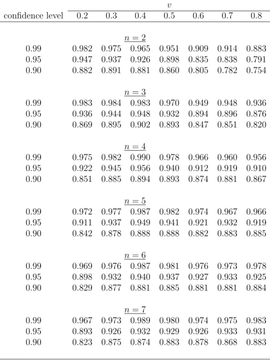
In the case of the Uniform [0,1] distribution (α = 1, Table S.1), we observe some deviation of the simulated coverage probabilities from the nominal values when the PDF is estimated near the upper boundary and the number of bidders is small (n= 2,3). There is also some deviation of the simulated coverage probabilities from the nominal values for large n and v near the lower boundary of the support. Thus, as one can expect the normal approximation may breakdown near the boundaries of the support. However, away from the boundaries, as the results in Table S.1 indicate, the

(5)

normal approximation works well and the simulated coverage probabilities are close to their nominal values.

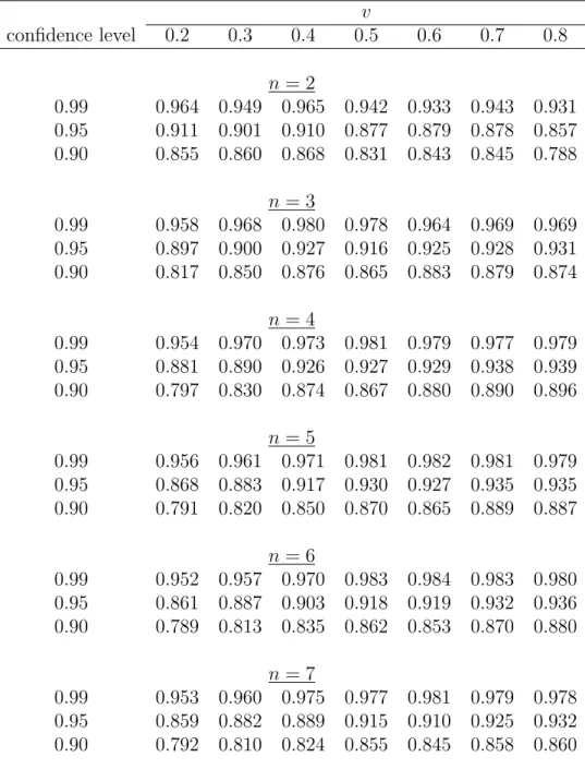
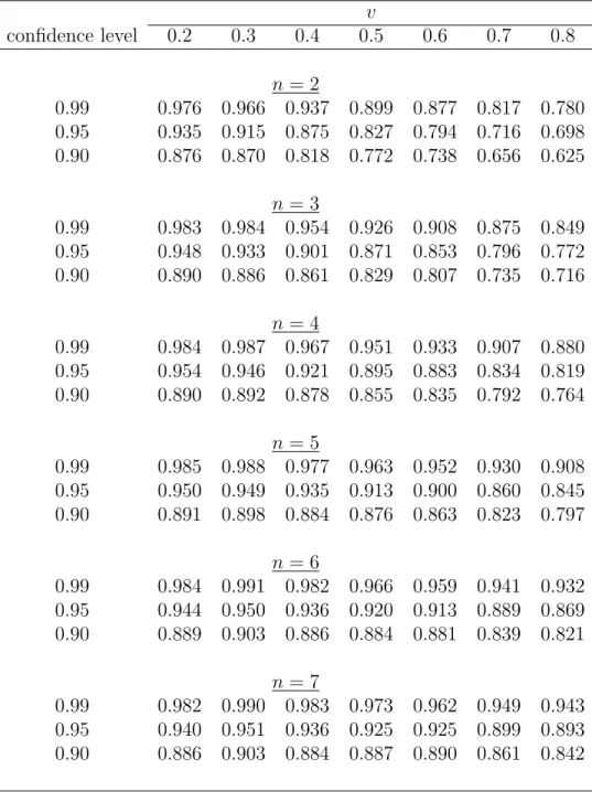
Similar results have been observed in the case of α = 2 (Table S.2) and α= 1/2 (Table S.3). When α = 2, the boundary effect distorting coverage probabilities is somewhat more pronounced near the lower boundary of the support, and less so near the upper boundary. An opposite situation is observed for α = 1/2: we see more distortion near the upper boundary and less near the lower boundary of the support. This can be explained by the fact that the PDF is increasing in the case ofα= 2, so there is relatively more mass nearv = 1, and it is decreasing when α= 1/2, so there is relatively less mass near v = 0. We observe good coverage probabilities away from the boundaries.

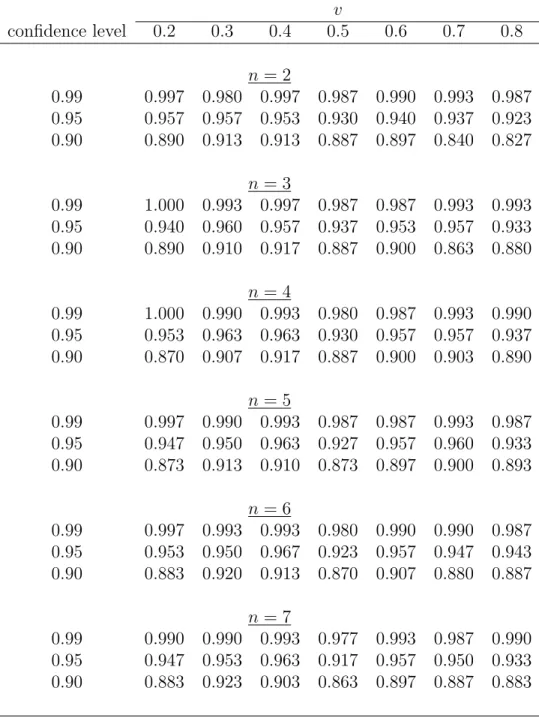
Tables S.4-S.6 report the coverage probabilities of the percentile bootstrap CIs. The bootstrap percentile confidence intervals are constructed as described in Section 4 in MS. The number of bootstrap samples used to compute φ†_τ in (23) in MS is

M = 199. The number of Monte Carlo replications used for the bootstrap experiments is 300.3 When α = 1, as reported in Table S.4, for the bootstrap percentile CIs we observe some size distortion only due to the right boundary effect and only for

n= 2. In all other cases, the bootstrap percentile CIs are found to be very accurate. With a few exceptions, the bootstrap percentile CIs outperform the CIs based on the traditional normal approximation.

Similar results are found for α = 2 and α = 1/2, see Tables S.5 and S.6. We find that the bootstrap percentile confidence intervals (CIs) have superior accuracy comparing to the CIs based on the traditional normal approximation. Based on these findings, we recommend using the bootstrap percentile method for the inference on the PDF of auction valuations.

We now turn to comparison of our estimator with the GPV’s estimator. Table S.7 reports the bias, MSE, and median absolute deviation of the two estimators for

α= 1. In most cases, the GPV’s estimator shows less bias. However neither estimator dominates the other in terms of MSE or median absolute deviation: our quantile-based (QB) estimator appears to be more efficient for small numbers of bidders (n = 2,3,4), and GPV’s is more efficient when n= 5,6, and 7. The GPV’s estimator is relatively more efficient when the PDF is upward sloping (α = 2) as the results Table S.8

3_{We use a smaller number of replications here because the bootstrap Monte Carlo simulations}

(6)

indicate. However, according to the results in Table S.9, the QB estimator dominates GPV’s in the majority of cases when the PDF is downward-sloping (α = 1/2).

Tables S.7, S.8, and S.9 also report the average (across replications) standard error for our QB estimator. The variance of the estimator increases with v, since it depends on F (v). This fact is also reflected in the MSE values that increase with v. Interestingly, one can see the same pattern for the MSE of the GPV estimator, which suggests that the GPV variance depends on v as well.

S.4 Proof of bootstrap Theorem 3 in MS

To simplify the notion, we will suppress the subscript indicating the bootstrap sample number for bootstrap objects (m). The bootstrap analogues of the original sample statistics are denoted by the superscript †.

We use Φ (·) to denote the standard normal CDF. Let P† denote probability conditional on the original sample {(b1l, . . . , bnll, nl, xl) : l = 1, . . . , L}. We say ζL =

o†_p(λL) ifP†(|ζL/λL|> ε)→p 0 for allε >0 asL→ ∞. We sayζL=Op†(λL) if for all

ε >0 there is ∆ε >0 such that for allL≥Lε,P(P†(|ζL/λL| ≥∆ε)> ε)< ε. We use

E†andV ar†to denote expectation and variance underP† respectively. Letπ†denote the distribution ofn†_l implied byP†, i.e. π†(n) = P†(n†_l =n) = L−1PL

l=11(nl=n) = ˆ

π(n), where π(n) = P(nl = n). Lastly, for two CDFs H1 and H2, let d∞(H1, H2)

denote the sup-norm distance between H1 _and _H2_:

d∞(H1, H2) = sup u∈R H1(u)−H2(u) .

Our proof uses the following two simple lemmas concerning the stochastic order (with respect toP†) of the bootstrap statistics. Let ˆθL be a statistic computed using

the data in the original sample, and let ˆθ†_L be the bootstrap analogue of ˆθL.

Lemma S.1 (a) Suppose that θˆL = θ+op(δL) and θˆ

†

L = ˆθL+o†p(δL). Then, θˆ

†

L =

θ+o†_p(δL).

(b) Suppose that θˆL=θ+Op(δL) and θˆ†_L= ˆθL+Op†(δL). Then, θˆ_L† =θ+O†p(δL).

Proof of Lemma S.1. For part (a), since ˆθL is not random under P†,

P†δ_L−1 ˆ θ†_L−θ > ε ≤P†δ−_L1 ˆ θL−θ > ε 2 +P†δ_L−1 ˆ θ_L† −θˆL > ε 2

(7)

= 1δ_L−1 ˆ θL−θ > ε 2 +op(1).

For the first summand, we have that for allε, η >0,

P1δ_L−1 ˆ θL−θ > ε 2 > η=P δ_L−1 ˆ θL−θ > ε 2 →0.

The proof of part (b) is similar.

Lemma S.2 Suppose that E†(ˆθ_L†)2 ₌_O

p(λ2L), then θˆ

†

L=O

†

p(λL).

Proof of Lemma S.2. Since E†(ˆθ_L†)2 ₌_O

p(λ2L), for all ε > 0 there is ∆ε >0 such

that P(E†(ˆθ_L†)2 _>_∆2

ελ2L)< ε. Let ˜∆2ε = ∆2ε/ε. Then, we can write

P(E†(ˆθ_L†)2 >∆˜2_εελ2_L)< ε (S.2)

for all L large enough. By Markov’s inequality,

P† ˆ θ_L† λL ≥∆˜ε ! ≤ E†θˆ†_L2 λ2 L∆˜2ε .

Thus, for all ε >0 there is ˜∆ε, such that for allL large enough,

P P† ˆ θ†_L λL ≥∆˜ε ! > ε ! ≤P    E†θˆ_L†2 ˜ ∆2 ελ2L > ε   < ε,

where the last inequality is by (S.2). Define

H_g,L† (u) =P† Lhd+31/2

ˆ

g†(1)(b|n, x)−gˆ(1)(b|n, x)

≤u,

Note thatH_g,L† (u) depends on x and b. We have the following result.

Lemma S.3 Let [b1(n, x), b2(n, x)] be as in (19) in MS. Suppose that Assumptions 1, 2, and 3 with k = 1 hold. Then, for all b ∈ [b1(n, x), b2(n, x)], x ∈ Interior(X) and n ∈ N, d∞(H_g,L† (u),Φ(u/Vg,1/12(b, n, x)))→p 0.

(8)

Proof of Lemma S.3. The result of the lemma follows from Theorem 1 in Mam-men (1992) since: (i) ˆg(1)₍_b_|_{n, x}_{) is a linear estimator; (ii) by Lemma 2(a) in MS,} (Lhd+3₎1/2_(ˆ_g(1)₍_b_|_{n, x}₎₋_g(1)₍_b_|_{n, x}₎₎ _→

d N(0, Vg,1(b, n, x)); (iii) d∞ is a metric; and

(iv) due to the under smoothing condition in Assumption 3.

Next, by the results in MS Lemma 1, Lemma S.1, and Lemma S.4 below, we have that for x∈Interior(X), n∈ N, and v ∈Λ(ˆ x),

ˆ

f†(v|n, x)−fˆ(v|x) = F (v|x)f

2₍_v_|_{n, x}₎

(n−1)g3₍_q₍_F₍_v_|_x₎_|_{n, x}₎_|_{n, x}₎

× gˆ†(1)(q(F (v|x)|n, x))−gˆ(1)(q(F(v|x)|n, x))+o†_p Lhd+3−1/2. (S.3) Note that by Lemma S.3 and (S.3),

H_f,L† (u)→p Φ

u V_f1/2(v, n, x)

!

,

where Vf(v, n, x) is defined in Theorem 2 in MS. Furthermore, by P´olya’s Theorem,

the convergence is uniform in u. The result of the theorem for H_f,L† then follows by the triangular inequality d∞(Hf,L, H

†

f,L)≤d∞(Hf,L,Φ) +d∞(H_f,L† ,Φ)→p 0.

Lemma S.4 Suppose that MS Assumptions 1, 2, and 3 with k = 1 hold. Then, for all x∈Interior(X) and n∈ N,

(e) sup_τ_∈_[0_,_1](limt↓τqˆ†(t|n, x)−qˆ†(τ|n, x)) =O†p

Lhd log(Lhd₎ −1 . (f ) sup_b_∈_[_b₁₍_n,x₎_,b₂₍_n,x_)]|ˆg(k)†₍_b_|_{n, x}₎₋_ˆ_g(k)₍_b_|_{n, x}₎_|₌_O† p Lhd+1+2k logL −1/2 , k = 0, . . . , R. (g) sup_τ∈[τ1−ε,τ2+ε]| ˆ Q†(τ|n, x)−Q(τ|x)|=O_p† Lhd+1 logL −1/2 +hR , for some ε >0 such that τ1−ε >0 and τ2+ε <1.

(9)

(h) sup_v_∈_Λ(ˆ _x₎|Fˆ†(v|n, x)−F (v|x)|=O†p Lhd+1 logL −1/2 +hR .

Proof of Lemma S.4. We prove part (b) first. Since (Lhd₎1/2_{( ˆ}_ϕ₍_x₎₋_Eϕ₍_x_{)) is} asymptotically normal by a standard result for kernel density estimators, by Theorem 1 in Mammen (1992), (Lhd)1/2 ϕˆ†(x)−ϕˆ(x) = O_p†(1). The result in part (b) follows.

For part (a), write

ˆ π(n|x) = ˆπ(n, x) ˆϕ(x) , where ˆ π(n, x) = 1 L L X l=1 1 (nl=n)Kh(x−xl).

By the same argument as in the proof of part (b), (Lhd₎1/2 _π_ˆ†₍_{n, x}₎₋_π_ˆ₍_{n, x}₎

is asymptotically normal. By the Taylor expansion of ˆπ†(n|x), the result in part (b), and since ˆϕ(x) is bounded away from zero with probability approaching one by As-sumption 1(b), Lhd1/2 πˆ†(n|x)−πˆ(n|x)= 1 ˆ ϕ(x) Lh d1/2 ˆ π†(n, x)−πˆ(n, x) −πˆ †₍_{n, x}₎ ( ˆϕ(x))2 Lh d1/2 ˆ ϕ†(x)−ϕˆ(x) +o Lhd1/2 ϕˆ†(x)−ϕˆ(x) =O_p†(1).

We prove part (c) next. The proof is based on the proof of Lemma B.1 in Newey (1994). For fixed x∈Interior(X) and n∈ N, write

ˆ G(bn, x) = ˆG(b|n, x) ˆπ(n|x) ˆϕ(x), so that ˆ G(b, n, x) = 1 nL L X l=1 nl X i=1 Til, with Til = 1 (bil ≤b) 1 (nl =n)K∗h(xl−x), (S.4)

(10)

and let ˆ G†(b, n, x) = 1 nL L X l=1 nl X i=1 T_il†(b), T_il†(b) = 1b†_il ≤b1n†_l =nK∗h x†_l −x.

Next, for chosen n and x, let

I =

b(n, x),¯b(n, x)

, I =∪JL

k=1Ik,

where the sub-intervals Ik’s are non-overlapping and of length

sL=

logL

L . (S.5)

Denote as ck the center of Ik. Note that I, Ik, ck depend onn and x. Denote as κ(b)

the interval containing b. Since

ˆ G(b, n, x) =E†T_il†(b), we can write ˆ G†(b, n, x)−Gˆ(b, n, x) =A†_L(b)−B_L† (b) +C_L†(b) , where A†_L(b) = 1 nL L X l=1 nl X i=1 T_il†(b)−T_il† cκ(b) , B_L†(b) = 1 nL L X l=1 nl X i=1 E†T_il†(b)−E†T_il† cκ(b) , C_L†(b) = 1 nL L X l=1 nl X i=1 T_il† cκ(b) −E†T_il† cκ(b) .

In the above decomposition, A†_L(b) is the average of the deviations of T_il†(b) from its value computed using the center of the interval containing b, and B_L†(b) is the expected value under P† of A†_L(b). The terms sup_b_∈_I|A†_L(b)| and sup_b_∈_I|B_L†(b)| are small when sL is small.

(11)

For A†_L we have T † il(b)−T † il cκ(b) ≤h−d(supK)d1n†_l =n 1 b†_il ≤b−1b†_il ≤cκ(b) ≤h−d(supK)d1n†_l =n1b†_il ∈Iκ(b) , (S.6) and therefore, A † L(b) ≤h −d_(sup_K₎d 1 nL L X l=1 n X i=1 1n†_l =n1b†_il ∈Iκ(b) . (S.7) Next, E† 1 nL L X l=1 n X i=1 1n†_l =n1b†_il ∈Ik −P†b†_il ∈Ik|n † l =n π†(n) !2 ≤ ≤ P†b†_il ∈Ik|n † l =n π†(n) nL , (S.8) and by Lemma S.2, 1 nL L X l=1 nl X i=1 1n†_l =n1b†_il ∈Ik =P†b†_il ∈Ik|n † l =n π†(n) +O_p†   P† b†_il ∈Ik|n†_l =n π†(n) L   1/2 =P†b†_il ∈Ik|n † l =n π†(n)   1 +O † p   1 P†_b† il ∈Ik|n † l =n π†₍_n₎_L   1/2  . (S.9)

Now, by a similar argument,

P† b†_il ∈Ik|n†_l =n π†(n) = 1 nL L X l=1 nl X i=1 1 (nl =n) 1 (bil ∈Ik)

(12)

=P(bil ∈Ik|nl =n)π(n) 1 +Op 1 P (bil ∈Ik|nl=n)π(n)L 1/2! ≤ sup k=1,...,JL P (bil ∈Ik|nl=n)π(n) × 1 +Op 1 infk=1,...,JLP (bil ∈Ik|nl =n)π(n)L 1/2! . (S.10)

Furthermore, for all Ik’s

inf b∈I,x∈Xg(b|n, x) sL≤P (bil ∈Ik|nl =n)≤ sup b∈I,x∈X g(b|n, x) sL. (S.11)

Equations (S.7)-(S.11) together imply that

sup b∈I A†_L(b) =O_p† h−dsL 1 +Op 1 sLL 1/2!! =O_p† logL Lhd , (S.12)

where the last equality is by (S.5).

By (S.6), (S.10), and (S.11), for B_L† (b) we have

sup b∈I B†_L(b) ≤sup b∈I E† T † il(b)−T † il cκ(b) ≤h−d(supK)dπ†(n) sup k=1,...,JL P†b†_il ∈Ik|n † l =n =O_p† logL Lhd . (S.13)

Note that C_L†(b) depends on b only through ck’s, and therefore

sup

b∈I

|C_L†(b)| ≤ max

k=1,...,JL

|C_L†(ck)|. (S.14)

A Bonferroni inequality implies that for any ∆>0,

P† Lhd logL 1/2 max k=1,...,JL |C_L†(ck)|>∆ ! ≤

(13)

≤ JL X k=1 P† L X l=1 nl X i=1 T_il†(ck)−E†T † il(ck) >∆nL logL Lhd 1/2! . (S.15) By (S.4), |T_il†(ck)| ≤h−d(supK)d and T † il(ck)−E†T † il(ck) ≤2(supK) d_h−d_.

Further, by (S.8)-(S.11), there is a constant 0< D1 <∞ such that

V ar†T_il†(ck) ≤D1h−2dsL(1 +op(1)) =D1h−d logL/ Lhd (1 +op(1)).

We therefore can apply Bernstein’s inequality (Pollard, 1984, page 193) to obtain

P† L X l=1 nl X i=1 T_il†(ck)−E†T † il(ck) >∆nL logL Lhd 1/2! ≤2 exp −1 2 ∆2n2L2 log_LhLd nLD1h−d(1 +op(1))log_LhdL + (2/3) ∆n(supK)dh−dL logL Lhd 1/2 ! = 2 exp −1 2 ∆2_n_(log_L₎1/2 _Lhd1/2 D1(logL/(Lhd)) 1/2 (1 +op(1)) + (2/3) ∆(supK)d ! = 2 exp − ∆n (4/3) (supK)d₊_o p(1) (logL)1/2 Lhd1/2 , (S.16)

where the equality in the last line is due to Lhd/logL → ∞. The inequalities in (S.14)-(S.16) together with (S.5) imply that there is a constant 0 < D2 < ∞ such that P† Lhd logL 1/2 sup b∈I |C_L†(b)|>∆ ! ≤2JLexp − ∆n (4/3) (supK)d₊_o p(1) (logL)1/2 Lhd1/2 ≤D2s−L1exp − ∆n (4/3) (supK)d₊_o p(1) (logL)1/2 Lhd1/2 ≤D2exp logL 1− ∆n (4/3) (supK)d₊_o p(1) Lhd logL 1/2!!

(14)

=op(1),

where the equality in the last line is by Lhd/logL → ∞. By a similar argument as in the proof of Lemma S.2,

sup b∈I |C_L†(b)|=o†_p Lhd logL −1/2 . (S.17)

The result of part (c) follows from (S.12), (S.13), and (S.17).

The proof of part (d) is similar to that of Lemma 1(d) in MS. First, by similar arguments as in the proof of Lemma 1(d), one can show that b(n, x) ≤ qˆ†(ε|n, x) ≤ ˆ

q†(1−ε|n, x)≤¯b(n, x) with probability P† approaching one (in probability). Second, one can show that uniformly overτ ∈[ε,1−ε],

ˆ G† qˆ†(τ|n, x)|n, x =τ +O†_p Lhd−1 Lastly, G qˆ†(τ|n, x)|n, x −Gˆ† qˆ†(τ|n, x)|n, x =G qˆ†(τ|n, x)|n, x−τ+O†_p Lhd−1 =G qˆ†(τ|n, x)|n, x−G(q(τ|n, x)|n, x) +O†_p Lhd−1 =g q˜†(τ|n, x)|n, x ˆ q†(τ|n, x)−q(τ|n, x) +O†_p Lhd−1 ,

where ˜q† denotes the mean value, or

ˆ q†(τ|n, x)−q(τ|n, x) = G qˆ †₍_τ_|_{n, x}_)|_{n, x} −Gˆ† qˆ†(τ|n, x)|n, x g(˜q†₍_τ_|_{n, x}₎_|_{n, x}₎ +O † p Lh d−1 = G qˆ †₍_τ_|_{n, x}_)|_{n, x} −Gˆ qˆ†(τ|n, x)|n, x g(˜q†₍_τ_|_{n, x}₎_|_{n, x}₎ + ˆ G qˆ†(τ|n, x)|n, x−Gˆ† qˆ†(τ|n, x)|n, x g(˜q†₍_τ_|_{n, x}₎_|_{n, x}₎ +O † p Lh d−1 ,

and the desired result follows.

The proof of part (e) is similar to that of Lemma 1(e). The proof of part (f) is similar to the proof of part (c) and relies on the fact that, according to Assumption

(15)

2 in MS, the derivatives ofK are Lipschitz. The proof of parts (g) and (h) is similar to that of Lemma 1(g) and (h).

References

Andrews, D. W. K., and J. H. Stock (2005): “Inference with Weak

Instru-ments,” Cowles Foundation Discussion Paper 1530, Yale University.

Chernozhukov, V., H. Hong, and E. Tamer (2007): “Estimation and

Confi-dence Regions for Parameter Sets in Econometric Models,” Econometrica, 75(5), 1243–1284.

Elliott, G., and U. K. M¨uller (2007): “Confidence Sets For the Date of a

Single Break in Linear Time Series Regressions,”Journal of Econometrics, 141(2), 1196–1218.

Guerre, E., I. Perrigne, and Q. Vuong (2000): “Optimal Nonparametric

Es-timation of First-Price Auctions,”Econometrica, 68(3), 525–74.

Haile, P. A., and E. Tamer (2003): “Inference with an Incomplete Model of

English Auctions,” Journal of Political Economy, 111(1), 1–51.

Lehmann, E. L., and J. P. Romano (2005): Testing Statistical Hypotheses.

Springer, New York, third edn.

Li, T., I. Perrigne, and Q. Vuong (2003): “Semiparametric Estimation of the

Optimal Reserve Price in First-Price Auctions,”Journal of Business & Economic Statistics, 21(1), 53–65.

Mammen, E. (1992): “Bootstrap, Wild Bootstrap, and Asymptotic Normality,”

Probability Theory and Related Fields, 93(4), 439–455.

Marmer, V., and A. Shneyerov (2010): “Quantile-Based Nonparametric

Infer-ence For First-Price Auctions,” Working Paper, University of British Columbia.

Myerson, R. B. (1981): “Optimal Auction Design,” Mathematics of Operations

(16)

Newey, W. K.(1994): “Kernel Estimation of Partial Means and a General Variance

Estimator,”Econometric Theory, 10(2), 233–253.

Paarsch, H. J. (1997): “Deriving an estimate of the optimal reserve price: An

application to British Columbian timber sales,” Journal of Econometrics, 78(2), 333–357.

Pollard, D. (1984): Convergence of Stochastic Processes. Springer-Verlag, New

York.

Riley, J., and W. Samuelson (1981): “Optimal auctions,” American Economic

(17)

Table S.1: Simulated coverage probabilities of the normal approximation CIs for the PDF of valuations for different points of density estimation (v), numbers of bidders (n) and auctions (L), sample size nL = 4200, and the distribution parameter α=1

(Uniform [0,1] distribution) v confidence level 0.2 0.3 0.4 0.5 0.6 0.7 0.8 n= 2 0.99 0.982 0.975 0.965 0.951 0.909 0.914 0.883 0.95 0.947 0.937 0.926 0.898 0.835 0.838 0.791 0.90 0.882 0.891 0.881 0.860 0.805 0.782 0.754 n= 3 0.99 0.983 0.984 0.983 0.970 0.949 0.948 0.936 0.95 0.936 0.944 0.948 0.932 0.894 0.896 0.876 0.90 0.869 0.895 0.902 0.893 0.847 0.851 0.820 n= 4 0.99 0.975 0.982 0.990 0.978 0.966 0.960 0.956 0.95 0.922 0.945 0.956 0.940 0.912 0.919 0.910 0.90 0.851 0.885 0.894 0.893 0.874 0.881 0.867 n= 5 0.99 0.972 0.977 0.987 0.982 0.974 0.967 0.966 0.95 0.911 0.937 0.949 0.941 0.921 0.932 0.919 0.90 0.842 0.878 0.888 0.888 0.882 0.883 0.885 n= 6 0.99 0.969 0.976 0.987 0.981 0.976 0.973 0.978 0.95 0.898 0.932 0.940 0.937 0.927 0.933 0.925 0.90 0.829 0.877 0.881 0.885 0.881 0.881 0.884 n= 7 0.99 0.967 0.973 0.989 0.980 0.974 0.975 0.983 0.95 0.893 0.926 0.932 0.929 0.926 0.933 0.931 0.90 0.823 0.875 0.874 0.883 0.878 0.868 0.883

(18)

Table S.2: Simulated coverage probabilities of the normal approximation CIs for the PDF of valuations for different points of density estimation (v), numbers of bidders (n) and auctions (L), sample size nL= 4200, and the distribution parameter α=2

v confidence level 0.2 0.3 0.4 0.5 0.6 0.7 0.8 n= 2 0.99 0.964 0.949 0.965 0.942 0.933 0.943 0.931 0.95 0.911 0.901 0.910 0.877 0.879 0.878 0.857 0.90 0.855 0.860 0.868 0.831 0.843 0.845 0.788 n= 3 0.99 0.958 0.968 0.980 0.978 0.964 0.969 0.969 0.95 0.897 0.900 0.927 0.916 0.925 0.928 0.931 0.90 0.817 0.850 0.876 0.865 0.883 0.879 0.874 n= 4 0.99 0.954 0.970 0.973 0.981 0.979 0.977 0.979 0.95 0.881 0.890 0.926 0.927 0.929 0.938 0.939 0.90 0.797 0.830 0.874 0.867 0.880 0.890 0.896 n= 5 0.99 0.956 0.961 0.971 0.981 0.982 0.981 0.979 0.95 0.868 0.883 0.917 0.930 0.927 0.935 0.935 0.90 0.791 0.820 0.850 0.870 0.865 0.889 0.887 n= 6 0.99 0.952 0.957 0.970 0.983 0.984 0.983 0.980 0.95 0.861 0.887 0.903 0.918 0.919 0.932 0.936 0.90 0.789 0.813 0.835 0.862 0.853 0.870 0.880 n= 7 0.99 0.953 0.960 0.975 0.977 0.981 0.979 0.978 0.95 0.859 0.882 0.889 0.915 0.910 0.925 0.932 0.90 0.792 0.810 0.824 0.855 0.845 0.858 0.860

(19)

Table S.3: Simulated coverage probabilities of the normal approximation CIs for the PDF of valuations for different points of density estimation (v), numbers of bidders (n) and auctions (L), sample sizenL = 4200, and the distribution parameterα=1/2

(20)

Table S.4: Simulated coverage probabilities of the bootstrap percentile CIs for PDF of valuations for different points of density estimation (v), numbers of bidders (n) and auctions (L), sample size nL = 4200, and the distribution parameter α=1

(Uniform [0,1] distribution) v confidence level 0.2 0.3 0.4 0.5 0.6 0.7 0.8 n= 2 0.99 0.997 0.980 0.997 0.987 0.990 0.993 0.987 0.95 0.957 0.957 0.953 0.930 0.940 0.937 0.923 0.90 0.890 0.913 0.913 0.887 0.897 0.840 0.827 n= 3 0.99 1.000 0.993 0.997 0.987 0.987 0.993 0.993 0.95 0.940 0.960 0.957 0.937 0.953 0.957 0.933 0.90 0.890 0.910 0.917 0.887 0.900 0.863 0.880 n= 4 0.99 1.000 0.990 0.993 0.980 0.987 0.993 0.990 0.95 0.953 0.963 0.963 0.930 0.957 0.957 0.937 0.90 0.870 0.907 0.917 0.887 0.900 0.903 0.890 n= 5 0.99 0.997 0.990 0.993 0.987 0.987 0.993 0.987 0.95 0.947 0.950 0.963 0.927 0.957 0.960 0.933 0.90 0.873 0.913 0.910 0.873 0.897 0.900 0.893 n= 6 0.99 0.997 0.993 0.993 0.980 0.990 0.990 0.987 0.95 0.953 0.950 0.967 0.923 0.957 0.947 0.943 0.90 0.883 0.920 0.913 0.870 0.907 0.880 0.887 n= 7 0.99 0.990 0.990 0.993 0.977 0.993 0.987 0.990 0.95 0.947 0.953 0.963 0.917 0.957 0.950 0.933 0.90 0.883 0.923 0.903 0.863 0.897 0.887 0.883

(21)

Table S.5: Simulated coverage probabilities of the bootstrap percentile CIs for PDF of valuations for different points of density estimation (v), numbers of bidders (n) and auctions (L), sample size nL= 4200, and the distribution parameter α=2

(22)

Table S.6: Simulated coverage probabilities of the bootstrap percentile CIs for PDF of valuations for different points of density estimation (v), numbers of bidders (n) and auctions (L), sample sizenL = 4200, and the distribution parameterα=1/2

(23)

Table S.7: Bias, MSE and median absolute deviation of the quantile-based (QB) and GPV estimators, and the average standard error (second-order corrected) of the QB estimator, for different points of density estimations (v), numbers of bidders (n) and auctions (L), sample size nL = 4200, and the distribution parameterα=1 (Uniform [0,1] distribution)

Bias MSE Med abs deviation

v QB GPV QB GPV QB GPV Std err QB n = 2 0.2 -0.0025 0.0030 0.0126 0.0218 0.0909 0.1186 0.1073 0.3 -0.0191 -0.0022 0.0216 0.0439 0.1178 0.1683 0.1519 0.4 -0.0173 0.0099 0.0405 0.0768 0.1556 0.2189 0.2004 0.5 -0.0270 0.0227 0.0560 0.1177 0.1801 0.2696 0.2471 0.6 -0.0743 -0.0068 0.0764 0.1571 0.2123 0.3141 0.2752 0.7 -0.0722 0.0195 0.1027 0.2061 0.2405 0.3681 0.3312 0.8 -0.0917 0.0061 0.2016 0.2366 0.2744 0.3959 0.4143 n = 3 0.2 0.0004 0.0025 0.0077 0.0082 0.0710 0.0731 0.0793 0.3 -0.0111 -0.0035 0.0114 0.0145 0.0851 0.0970 0.1073 0.4 -0.0063 0.0045 0.0194 0.0245 0.1094 0.1245 0.1382 0.5 -0.0056 0.0147 0.0284 0.0371 0.1299 0.1522 0.1701 0.6 -0.0342 -0.0059 0.0402 0.0519 0.1556 0.1813 0.1947 0.7 -0.0264 0.0114 0.0503 0.0720 0.1781 0.2161 0.2287 0.8 -0.0433 0.0017 0.0613 0.0857 0.1953 0.2372 0.2578 n = 4 0.2 0.0013 0.0021 0.0059 0.0050 0.0619 0.0567 0.0667 0.3 -0.0084 -0.0039 0.0077 0.0077 0.0697 0.0696 0.0860 0.4 -0.0031 0.0023 0.0121 0.0124 0.0871 0.0886 0.1079 0.5 0.0004 0.0110 0.0175 0.0183 0.1033 0.1071 0.1311 0.6 -0.0204 -0.0044 0.0248 0.0256 0.1226 0.1275 0.1505 0.7 -0.0115 0.0082 0.0315 0.0360 0.1415 0.1514 0.1764 0.8 -0.0233 0.0002 0.0380 0.0429 0.1545 0.1660 0.1982

(24)

Table S.7: Continued (α=1)

v QB GPV QB GPV QB GPV Std err QB n = 5 0.2 0.0016 0.0019 0.0050 0.0037 0.0570 0.0490 0.0600 0.3 -0.0072 -0.0040 0.0060 0.0052 0.0611 0.0565 0.0741 0.4 -0.0017 0.0013 0.0087 0.0078 0.0744 0.0703 0.0905 0.5 0.0026 0.0088 0.0124 0.0113 0.0877 0.0843 0.1083 0.6 -0.0138 -0.0035 0.0171 0.0156 0.1026 0.0997 0.1241 0.7 -0.0051 0.0064 0.0220 0.0217 0.1182 0.1170 0.1444 0.8 -0.0147 -0.0003 0.0262 0.0259 0.1278 0.1284 0.1615 n = 6 0.2 0.0018 0.0018 0.0046 0.0032 0.0540 0.0448 0.0560 0.3 -0.0065 -0.0040 0.0051 0.0039 0.0559 0.0493 0.0667 0.4 -0.0010 0.0007 0.0069 0.0057 0.0665 0.0598 0.0795 0.5 0.0037 0.0074 0.0096 0.0079 0.0774 0.0708 0.0937 0.6 -0.0101 -0.0029 0.0129 0.0108 0.0895 0.0831 0.1068 0.7 -0.0020 0.0053 0.0167 0.0148 0.1026 0.0961 0.1231 0.8 -0.0100 -0.0005 0.0195 0.0175 0.1105 0.1055 0.1374 n = 7 0.2 0.0019 0.0017 0.0043 0.0028 0.0522 0.0423 0.0535 0.3 -0.0061 -0.0040 0.0045 0.0033 0.0526 0.0449 0.0618 0.4 -0.0006 0.0004 0.0059 0.0045 0.0613 0.0533 0.0721 0.5 0.0042 0.0064 0.0079 0.0061 0.0704 0.0620 0.0836 0.6 -0.0077 -0.0024 0.0103 0.0082 0.0805 0.0723 0.0947 0.7 -0.0004 0.0045 0.0133 0.0109 0.0917 0.0824 0.1082 0.8 -0.0075 -0.0005 0.0152 0.0128 0.0977 0.0903 0.1202

(25)

Table S.8: Bias, MSE and median absolute deviation of the quantile-based (QB) and GPV estimators, and the average standard error (second-order corrected) of the QB estimator, for different points of density estimations (v), numbers of bidders (n) and auctions (L), sample size nL = 4200, and the distribution parameterα=2

v QB GPV QB GPV QB GPV Std err QB n = 2 0.2 -0.0024 0.0008 0.0043 0.0048 0.0508 0.0555 0.0588 0.3 -0.0153 -0.0056 0.0126 0.0159 0.0867 0.1010 0.1028 0.4 -0.0144 0.0053 0.0268 0.0337 0.1257 0.1465 0.1596 0.5 -0.0380 -0.0097 0.0477 0.0620 0.1702 0.1983 0.2173 0.6 -0.0443 0.0027 0.0727 0.1015 0.2129 0.2588 0.2855 0.7 -0.0562 0.0197 0.1197 0.1621 0.2602 0.3228 0.3617 0.8 -0.0912 -0.0110 0.2400 0.2360 0.3379 0.3920 0.4430 n = 3 0.2 -0.0013 0.0003 0.0022 0.0019 0.0377 0.0346 0.0391 0.3 -0.0072 -0.0034 0.0057 0.0051 0.0595 0.0569 0.0660 0.4 -0.0037 0.0028 0.0113 0.0106 0.0837 0.0817 0.0995 0.5 -0.0166 -0.0084 0.0194 0.0188 0.1116 0.1091 0.1345 0.6 -0.0137 0.0029 0.0310 0.0299 0.1401 0.1404 0.1779 0.7 -0.0103 0.0133 0.0499 0.0478 0.1716 0.1735 0.2242 0.8 -0.0384 -0.0052 0.0730 0.0733 0.2136 0.2172 0.2656 n = 4 0.2 -0.0012 0.0001 0.0018 0.0013 0.0337 0.0288 0.0332 0.3 -0.0049 -0.0024 0.0039 0.0029 0.0494 0.0431 0.0523 0.4 -0.0015 0.0018 0.0071 0.0057 0.0669 0.0602 0.0755 0.5 -0.0103 -0.0066 0.0113 0.0095 0.0858 0.0779 0.1007 0.6 -0.0065 0.0019 0.0182 0.0150 0.1077 0.0990 0.1311 0.7 -0.0015 0.0099 0.0281 0.0232 0.1309 0.1207 0.1637 0.8 -0.0186 -0.0037 0.0423 0.0356 0.1623 0.1507 0.1957

(26)

Table S.8: Continued (α=2)

v QB GPV QB GPV QB GPV Std err QB n = 5 0.2 -0.0012 -0.0001 0.0016 0.0011 0.0322 0.0265 0.0311 0.3 -0.0039 -0.0019 0.0032 0.0022 0.0447 0.0376 0.0459 0.4 -0.0008 0.0014 0.0054 0.0040 0.0585 0.0503 0.0635 0.5 -0.0075 -0.0054 0.0080 0.0062 0.0721 0.0629 0.0831 0.6 -0.0041 0.0011 0.0127 0.0097 0.0905 0.0794 0.1062 0.7 0.0012 0.0079 0.0190 0.0144 0.1085 0.0949 0.1312 0.8 -0.0120 -0.0030 0.0277 0.0217 0.1320 0.1172 0.1566 n = 6 0.2 -0.0014 -0.0002 0.0016 0.0011 0.0315 0.0255 0.0302 0.3 -0.0033 -0.0016 0.0028 0.0019 0.0424 0.0347 0.0426 0.4 -0.0006 0.0011 0.0046 0.0032 0.0538 0.0451 0.0569 0.5 -0.0058 -0.0046 0.0064 0.0047 0.0641 0.0547 0.0729 0.6 -0.0030 0.0006 0.0100 0.0072 0.0800 0.0683 0.0914 0.7 0.0023 0.0066 0.0144 0.0103 0.0947 0.0804 0.1115 0.8 -0.0087 -0.0026 0.0203 0.0151 0.1134 0.0975 0.1324 n = 7 0.2 -0.0014 -0.0002 0.0016 0.0010 0.0312 0.0249 0.0299 0.3 -0.0029 -0.0014 0.0026 0.0017 0.0411 0.0331 0.0407 0.4 -0.0004 0.0009 0.0041 0.0028 0.0509 0.0421 0.0529 0.5 -0.0048 -0.0040 0.0055 0.0039 0.0591 0.0497 0.0664 0.6 -0.0024 0.0001 0.0084 0.0058 0.0732 0.0613 0.0818 0.7 0.0028 0.0057 0.0117 0.0080 0.0858 0.0713 0.0986 0.8 -0.0068 -0.0023 0.0161 0.0115 0.1011 0.0848 0.1163

(27)

Table S.9: Bias, MSE and median absolute deviation of the quantile-based (QB) and GPV estimators, and the average standard error (second-order corrected) of the QB estimator, for different points of density estimations (v), numbers of bidders (n) and auctions (L), sample size nL = 4200, and the distribution parameterα=1/2

v QB GPV QB GPV QB GPV Std err QB n= 2 0.2 -0.0186 -0.0102 0.0220 0.0576 0.1195 0.1891 0.1497 0.3 -0.0201 0.0018 0.0343 0.1059 0.1479 0.2512 0.1886 0.4 -0.0458 -0.0190 0.0706 0.1409 0.1737 0.2902 0.2269 0.5 -0.0625 0.0010 0.0548 0.1800 0.1790 0.3330 0.2486 0.6 -0.0706 -0.0137 0.5800 0.1700 0.2100 0.3238 0.7302 0.7 -0.1047 0.0020 0.0756 0.1771 0.2107 0.3397 0.2954 0.8 -0.1042 0.0107 0.2375 0.1719 0.2342 0.3332 0.5659 n= 3 0.2 -0.0124 -0.0040 0.0144 0.0241 0.0976 0.1247 0.1194 0.3 -0.0110 -0.0009 0.0213 0.0412 0.1163 0.1631 0.1463 0.4 -0.0302 -0.0110 0.0299 0.0572 0.1353 0.1892 0.1694 0.5 -0.0323 0.0030 0.0352 0.0770 0.1482 0.2242 0.1963 0.6 -0.0596 -0.0094 0.0393 0.0781 0.1518 0.2214 0.2091 0.7 -0.0763 0.0053 0.1213 0.0948 0.1771 0.2495 0.2785 0.8 -0.0742 0.0149 0.0984 0.0997 0.1841 0.2539 0.2962 n= 4 0.2 -0.0089 -0.0006 0.0109 0.0136 0.0848 0.0946 0.1017 0.3 -0.0070 -0.0004 0.0146 0.0219 0.0969 0.1193 0.1212 0.4 -0.0199 -0.0072 0.0206 0.0308 0.1140 0.1393 0.1399 0.5 -0.0146 0.0032 0.0278 0.0418 0.1287 0.1653 0.1646 0.6 -0.0393 -0.0061 0.0284 0.0432 0.1301 0.1662 0.1750 0.7 -0.0438 0.0048 0.0469 0.0565 0.1466 0.1927 0.2027 0.8 -0.0530 0.0128 0.0455 0.0627 0.1534 0.2018 0.2164

(28)

Table S.9: Continued (α=1/2)

v QB GPV QB GPV QB GPV Std err QB n = 5 0.2 -0.0067 0.0015 0.0089 0.0092 0.0768 0.0780 0.0903 0.3 -0.0046 0.0004 0.0110 0.0137 0.0842 0.0946 0.1048 0.4 -0.0142 -0.0053 0.0156 0.0195 0.0992 0.1106 0.1201 0.5 -0.0077 0.0035 0.0208 0.0261 0.1130 0.1304 0.1400 0.6 -0.0278 -0.0039 0.0211 0.0273 0.1136 0.1320 0.1500 0.7 -0.0299 0.0037 0.0292 0.0366 0.1277 0.1549 0.1699 0.8 -0.0363 0.0102 0.0329 0.0419 0.1353 0.1649 0.1838 n = 6 0.2 -0.0052 0.0028 0.0076 0.0069 0.0712 0.0678 0.0824 0.3 -0.0030 0.0012 0.0087 0.0096 0.0753 0.0792 0.0934 0.4 -0.0107 -0.0042 0.0124 0.0136 0.0886 0.0925 0.1059 0.5 -0.0046 0.0037 0.0162 0.0180 0.1005 0.1079 0.1221 0.6 -0.0206 -0.0026 0.0164 0.0189 0.1009 0.1097 0.1316 0.7 -0.0213 0.0029 0.0216 0.0255 0.1142 0.1291 0.1478 0.8 -0.0257 0.0084 0.0249 0.0295 0.1206 0.1383 0.1601 n = 7 0.2 -0.0041 0.0038 0.0068 0.0056 0.0672 0.0611 0.0767 0.3 -0.0019 0.0018 0.0073 0.0072 0.0689 0.0688 0.0851 0.4 -0.0086 -0.0034 0.0103 0.0101 0.0806 0.0800 0.0954 0.5 -0.0029 0.0037 0.0131 0.0132 0.0907 0.0925 0.1088 0.6 -0.0159 -0.0019 0.0132 0.0139 0.0908 0.0940 0.1176 0.7 -0.0156 0.0025 0.0171 0.0188 0.1027 0.1106 0.1313 0.8 -0.0185 0.0072 0.0202 0.0218 0.1094 0.1186 0.1427