414
Creative Construction Conference 2014
Singularity functions as new tool for integrated project
management
Gunnar LUCKO
1*and Yi SU
11
Department of Civil Engineering, Catholic University of America, 620 Michigan Avenue NE, Washington, DC 20064, USA
Abstract
Construction managers must actively plan and control the plethora of quantitative and qualitative aspects of their projects in a coordinated, judicious manner to achieve successful performance. However, current managerial techniques are compartmentalized into modeling and analyzing time, budget, resource utilization, equipment operations, and others. Therefore, the objective of this research is to explore how such very disparate aspects, here limited in scope to quantitative ones, can be integrated into a cohesive and versatile model. Its methodology is to adopt and adapt a traditional model from structural engineering called singularity functions. Generalizing elements of conventional algebra, they activate the non-zero behavior of their dependent variable over a specific range of one or several independent variables. Thus it is possible to model different relationships of project performance. Yet this accomplishment in analytical capability has left unsolved the issue of interfaces between said compartmentalized aspects. To address it, interactions between the pairwise work quantity, time, cost, and resource variables are explored and conversions between their respective input and output data are derived. The contribution of this research is threefold: First, the mathematical models of linear schedules, cash flows, and resources are aligned. Second, interactions between those models are extracted and formalized based on a common irreversible variable, which is time. Third, the possibility of integrating elements into a 3D or indeed nD quantitative model for project management is discussed. In conclusion, such integrated model based on singularity functions opens new possibilities for holistic planning and management of construction projects. Linking its various quantitative elements thus enables a customizable and easily adoptable approach and facilitates comprehensive analysis and multi-objective optimization toward minimum duration and cost and maximum resource utilization.
Keywords: Cash flows; integrated project management; quantitative performance measures; scheduling; singularity functions.
1.Introduction
Construction project management is a complex system, as it is driven by multiple objectives; “[t]hese objectives and their relative importance vary from one project to another, and they often include minimizing construction time and cost while maximizing safety, quality, and sustainability” (Kandil et al. 2010, p. 17). The term ‘objective’ can also be used interchangeably to the term dimension, as traditional project management is commonly defined as a three-dimensional (3D) cost-schedule-technical system (Gransberg et al. 2013). To handle the characteristics of such a complex system, previous studies divided construction projects into various subsystems. They typically focused on one compartmentalized subsystem as their research purpose, while simplifying or even omitting interfaces to other subsystems. For example, Gantt bar charts are a graphical scheduling method that is oriented exclusively toward the time dimension, ignoring others such as work quantity, cost, and resources. The well-known Critical Path Method (CPM) was developed for the requirement that “[t]he plan should point directly to the difficult and significant activities – the problems of achieving the objective” (Kelley and Walker 1959, p. 160). CPM may be described as a one-and-a-half dimensional method, because it primarily applies an algorithm to schedule time, while a separate later time-cost tradeoff analysis could consider direct cost, but not indirect cost (Kelley and Walker 1959). More recently, additional dimensions (often three) are brought into multi-objective models. They were solved “using a variety of methods, including linear programming, integer programming, dynamic programming, and genetic algorithms” (El-Rayes and Kandil 2005, p. 477). However, CPM still dominates as their limiting foundation, to the detriment of other dimensions. Yet construction projects are integrated systems that unfold in a complex interplay subject to a plethora of factors, which requires using a more integrated model to generate realistic analyses and efficient optimization. A need therefore exists to explore novel approaches toward such an integrated systems view of project management.
* Corresponding author. Tel.: 001-202-319-4381; fax: 001-202-319-6677. E-mail address: [email protected]
415
2.Literature ReviewTraditional research “selected [the] most important objective while either neglecting the less important competing objectives or imposing them as known constraints in the optimization formulation” (Wu et al. 2012, p. 1411). Such studies on single objectives usually explore a detailed subsystem, e.g. scheduling (Harris and Ioannou 1998) or cash flows (Cui et al. 2010). But construction projects are complex systems and thus it is deplorable that there exists “a plethora of “control” techniques that cannot provide any insight into the interactions among the many components of a construction engineering project” (Kalu 1990, p. 494). To manage multi-objective problems, studies seek to create “tools and strategies that can simultaneously improve project performance in multiple dimensions” for integrated systems (Ford 2002, p. 30). Yet “[m]ultiobjective optimization formulations have clear theoretical advantages but increase the complexity of the mathematical formulation” (Wu et al. 2012, p. 1411). In most cases, researchers make approximations to simplify the problem. Ammar (2011, p. 67) for the example of a time-cost tradeoff optimization explained that a “[d]iscount factor in the exponential form…, is too complicated to be handled in a mathematical optimization model… Instead, a simplified form… will be used.” Such approach is common in multi-objective research for reasons of simplicity, manageability, and brevity of a model and its description, but clearly undesirable.
Furthermore, such studies typically follow very similar steps: First, selecting objectives from project performance parameters to be minimized or maximized, e.g. time, cost, or resources. Second, using a multi-objective optimization algorithm. However, an important intermediate step is often short-changed, that of creating a model whose nature is ideally suited to its challenge. It logically occurs between establishing the objectives and performing an optimization and is crucial for an efficient and reliable optimization. Models must be versatile yet accurate to the maximum extent that input data allow, without imposing extraneous restrictions from modeling assumptions. Previous studies have focused extensively on optimization algorithms (Geem 2010), but appear to overlook this modeling challenge.
2.1.Research Need and Objectives
Abridged objective functions to minimize or maximize dependent variables radically simplify reality: Duration is determined by factors such as productivity, crew size, resource availability, shifts, lead/lag durations, buffers, etc.; multi-objective studies omit most such details. Cash flows must consider direct and indirect cost, bill-to-pay delay, prompt payment discount, credit limit, interest, time value of money, etc. Objective functions typically simplify these details, focusing instead on algorithms to identify or compare solutions. One may argue that it is overly complicated to maintain the same level of detail as local subsystems when moving to modeling a global integrated system. But per the paradigm of Ockham’s razor, who advocated ‘as simple as possible, as complicated as necessary’ for models, one should not reduce realism if a system becomes more complex, which limits the validity of its output and may mislead decision-makers. This research thus raises the fundamental question of how to bridge local and global views, while remaining efficient and accurate as determined by the quality of available data, not model assumptions. Singularity functions, defined in the following section, offer the unique features of detailability (can reflect any desired level of detail within their mathematical expressions),
extensibility (can incorporate any number of interacting dimensional variables), and convertibility (can extract pairwise performance parameters to examine their relationships in detail).
Three sequential Research Objectives will be addressed by this research, which together contribute to its overall goal of ultimately gaining a single comprehensive yet customizable approach to construction project management:
• Exploring interactions and conversions among singularity functions for merging subsystems into a global model;
• Aligning subsystem models of schedule, cash flows, and resources in cumulative and non-cumulative expressions;
• Visualizing the integrated 3D project model and assessing its potential contribution as a novel management tool.
3.Singularity Functions
Singularity functions were initially used in structural engineering to analyze the problem of beams that are loaded with diverse types of loads, which are located at discrete or distributed locations on said beams. The basic term of Equation 1 was historically known as the Föppl symbol (1927) or Macaulay brackets (1919). This operator performs a case distinction for the given cutoff value a of the independent variable x: The functions yields zero if x is smaller than a, while evaluating the pointed brackets as round ones if x is equal to or larger
416
than a. The strength s amplifies the value of the function, while the exponent n modifies the behavior to linear or nonlinear growth of the function.
The virtue of singularity functions is that they can easily model influences that are located at or distributed along a dimension (e.g. time), which fulfills requirements of various key applications in the construction management field. For example, in linear schedules, activity progress is represented as a curve with start and finish date, whose slope is the productivity. Moreover, for cash flows, a cost profile also has a start and finish; its slope is the rate at which the cost grows. Furthermore, for resources utilization, a profile can be derived analogously. Of course, multiple effects of the same type can be expressed jointly, which generates a staggered profile over its respective time period. All of such phenomena can be modeled with the basic term of singularity functions by inserting the respective appropriate independent and dependent variables per Table 1. This feature enables the conversion per Research Objective 1: Introducing a new variable, e.g. a cost factor for work units into a linear schedule, transforms the model as desired.
Table 1. Variables for singularity functions.
(
)
≥ − ⋅ < = − ⋅ a x for a x s a x for a x s n 0 n (1)Type of problem Independent Dependent Linear schedule x = work unit y = time unit Cash flows y = time unit z = cost unit Resource utilization y = time unit r = resource unit
3.1.Linear Schedule Model (cumulative and non-cumulative forms)
Most construction projects, whether pipelines or multi-floor buildings, contain many repeating activities (Harris and Ioannou 1998). CPM can only guarantee that sequential relations between those repeating activities are obeyed, but cannot directly represent constraints for resource continuity (Harris and Ioannou 1998), nor exploit the repetitive nature for the model itself. On the other hand, the Linear Scheduling Method (LSM) and closely related approaches with similar names, e.g. repetitive or location-based scheduling, which “analyze projects that are characterized as geometrically linear or repetitive in their operations” (Lucko 2008, p. 711), are able to take advantage of prevailing repetitiveness to derive a more intuitive model. It was widely considered to be merely graphically-based scheduling that “is presented graphically as an X-Y plot where one axis represents [repeating] units, and the other time” (Harris and Ioannou 1998, p. 270). Such graphical, non-mathematical focus was a severe limitation of LSM and has hindered its computerization and broader application in the construction industry. However, that situation has changed through the introduction of the Productivity Scheduling Method (PSM) that is based on singularity functions. They “provide a flexible and powerful mathematical model for construction activities and their buffers that are characterized by their linear or repetitive nature” (Lucko 2008, p. 711). Yet the fundamental mathematical connection between CPM and LSM remains largely unexplored, and – once understood – could facilitate broadening the capabilities of PSM.
Lucko (2009) described the steps of PSM as activity and buffer equations, initial stacking, minimum differences and differentiation for consolidation, which generates revised activity and buffer equations, and criticality analysis. Details of these steps are omitted in this paper for brevity. Stacking generates a feasible but extremely conservative and thus lengthy schedule, consolidation overlaps as many activities as possible within the sequence constraints. The approach of PSM is to convert all inputs about activity sequence, durations, leads or lags between activities, and any time or work break into the mathematical model that is composed of singularity functions. The schedule (start and finish of each activity in the initial and final versions) and its criticality characteristics are outputs. Time (y) is the independent variable in PSM per Equation 2, x is work, Ui is
the number of repeating work units, Di is the duration of activity i,
*
Si
a and a*Fi are its start and finish, whose asterisk indicates that they may include a shifted start (prior delay d1) or extended duration (new delay d2). Note
that time is better measured on the y-axis, because it should be minimized by the algorithm. An analogous form with time as the dependent variable can be derived by switching the axes. An example with activities A, B, and C
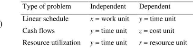
per Table 2 is shown in the x(y)-oriented linear schedule of Figure 1.
Figure 1 shows the schedule in a cumulative form, which means that the work quantity of each activity (vertical axis) increases with time that passes (horizontal axis). According to calculus, calculating the derivative of a function yields its rate of change (Strang 2010). Thus differentiating the cumulative Equation 2 returns the
non-cumulative Equation 3. Figure 2 shows this cumulative form. Interestingly, the profile of non-cumulative activity equations is similar to a traditional bar chart. It differs from a bar chart only in that the vertical axis represents productivity and not just an activity name or label. It thus displays more information than a bar chart. The activity with the highest productivity is placed at the top, and the smaller the productivity the lower the height where activity bars are placed.
417
( )
⋅ − − − −(
+)
⋅ − + = * 0 2 1 * 1 * 2 Fi i i Fi Si i i i i y a y a D d y a d D U y x (2)( )
⋅ − − − + = ′ * 0 * 0 2 Fi Si i i i i y a y a d D U y x (3)Table 2. Schedule, cash flow, and resource input for example. Name [-] Successor [-] Duration [months] Work Unit [count] Time Buffer [months] Shift d1 [months] Delay d2 [months] Cost C [$1000] Markup M [% of cost] Bill-to-Pay Delay b [months] Resource Rate [workers] A B 3 3 1 0 1 100 15 1 10 B C 9 3 2 1 0 200 10 1 20 C - 6 3 1 1 1 100 10 1 10
Figure 1. Cumulative linear schedule for example. Figure 2. Non-cumulative linear schedule for example.
Overall, PSM with its systematic application of singularity functions provides a mathematical model that unifies compartmentalized concepts and project performance parameters, as used e.g. in minimizing the project duration and determining the criticality of activities under CPM, displaying graphically their start and finish dates as in bar charts, and representing the starts, finishes, sequence, and productivity of activities as under LSM. The cumulative and non-cumulative forms of the equations enhance scheduling research in that it becomes apparent that concepts whose relation was previously arduous to express can indeed be explicitly modeled in such integrated quantitative manner.
3.2.Cash Flow Model (cumulative and non-cumulative forms)
The success or failure of construction projects strongly depends on cash flow management. Therefore, modeling cash flows is a crucial problem in construction management. However, it is a thorny problem, because the interaction of cash outflows and inflows generates a zigzag-shaped balance that used to defy modeling attempts until recently (Lucko 2011a). Moreover, some phenomena related to cash flows exhibit a distinct periodicity (Su and Lucko 2013), which should be modeled. Furthermore, Time Value of Money (TVM) can be considered explicitly (Lucko 2013).
Expanding the example from the previous section, assume that cost for each activity grows linearly (Elazouni and Metwally 2005). Table 2 lists the cost (C), markup (M), and bill-to-pay-delay (b) for each activity. Whereas the slope represented productivity in the linear schedule, the scale factor (C / (D + d2)) in the singularity function
per Equation 4 represents the rate of cost growth, which is the slope of the cost profile. Adding the markup to the cost yields a bill function per Equation 5. As bills are sent to the payer at the end of each period, an operator that rounds down the operand to its nearest integer is applied to the independent variable y. Such rounding operator can easily express the “periodicity [that] occurs both in cash outflows and inflows that have a specific frequency and amplitude, e.g., overhead, billing, and payment functions” (Lucko 2011a, p. 528). The pay function per Equation 6 is derived from the bill function, but subtracts the bill-to-pay-delay b from each y, which has the effect of moving the bill profile to the right to become the pay profile per Figure 3. Note that the cost, bill, pay, and balance profiles in Figure 3 model the entire project, adding the cash flows of the three activities accordingly. The balance is the difference between the sum of the cost functions (outflows) and the sum of all pay functions (inflows) per Equation 7. In a real project, b will be approximately 30 to 90 days; here it is assumed as one month. It is assumed that the balance function does not consider TVM. Its value depends on the period over which it is assessed, e.g. for financing interest or an unused credit fee, as analyzed in detail (Lucko 2011a, Lucko 2013, Su and Lucko 2013), but is excluded here for brevity.
x(y)C x(y)B x(y)A Work [quantity] Time [months] x’(y)C x’(y)B x’(y)A Time [months] Productivity [quantity/months]
418
Previous cash flow models are cumulative, yet the non-cumulative form of such cash flow models can also exist per Figure 4. Differentiating Equation 4 yields the non-cumulative cost function per Equation 8. A cumulative pay function has a stepped profile per Figure 3. Differentiating it would generate a bar chart-like profile, which would be incorrect, because the non-cumulative pay function should only be active at each pay. Su and Lucko (2013) solved this problem by introducing customized pay and signal functions for a non-cumulative bill per Equations 9 and 10.
( )
⋅ − − − + = * 1 * 1 2 Fi Si i i i i st co y a y a d D C y z (4)( )
(
)
⋅
− −
− + + = * 1 * 1 2 1 Fi Si i i i i i bill y a y a d D M C y z (5)( )
(
)
⋅
−
− −
−
− + + = * 1 * 1 2 1 Fi Si i i i i i pay y b a y b a d D M C y z (6)( )
( )
( )
i t s co i pay balance y z y z y z =∑ −∑ (7)( )
⋅ − − − + = ′ * 0 * 0 2 Fi Si i i i i st co y a y a d D C y z (8)( )
∑(
)
⋅( )
+ + ⋅ = z y d D M C y z pay signal i i i i pay each _ 2 _ 1 (9)( )
(
)
(
)
(
)
(
)
+ + − − + + − − + − − + − = * 1 * 1 * 1 * 1 _ y y a b y a b y a b 1 y a b 1 zpay signal s F s F (10)Figure 3. Cumulative cash flow profile for example. Figure 4. Non-cumulative cash flow profile for example.
3.3.Resource Model (cumulative and non-cumulative forms)
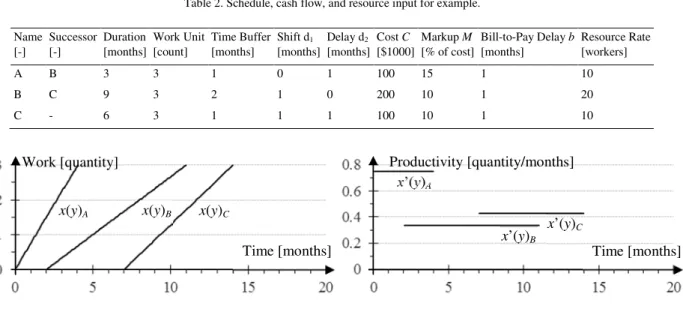
The same approach as described for linear scheduling and cash flows can also be adopted for resource utilization. Its scale factor per Equation 11 represents the rate of resource consumption r (Lucko 2011b), typically for general or specialized labor. Continuing the previous example, Table 2 lists the resource rate for each activity. Equations 11 and 12 express the cumulative and non-cumulative resource functions, respectively, which are shown in Figures 5 and 6.
Aligning these subsystems in their cumulative and non-cumulative forms fulfills Research Objective 2. Note that additional refinements can be added to reflect the aforementioned factors such as shifts d1 (that move the
start) and delays d2 (that move the finish, i.e. expand duration) (Lucko 2008) to enhance its realism. This can be
accomplished by adding them to the cutoff of the singularity function. Equation 13 links subsystems via the scaling factors of their pairwise variables for proportionality, notwithstanding further the moving and rounding the cutoff in bill equations.
Figure 5. Cumulative resource profile for example. Figure 6. Non-cumulative resource profile for example.
zbill(y) Cost [$1,000] Time [months] zcost(y) zpay(y) zbal(y) z’cost(y)
Cost Rate [$1,000 / month]
Time [months]
zeach_pay(y)
zbal(y)
r(y)A’
Resource Rate [workers / month]
Time [months] r(y)C’ r(y)B’ r(y)tot’ r(y)A Resources [workers] Time [months] r(y)C r(y)B r(y)tot
419
( )
= ⋅ − − − −(
+)
⋅ − * 0 2 1 * 1 * 3 i F F S i i s y a y a d y a y r (11)( )
− − − ⋅ = ′ * 0 * 0 F S i i s y a y a y r (12)(
)
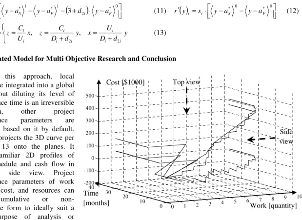
+ = + = = = y d D U x y d D C z x U C z z y x f i i i i i i i i 2 2 , , , , (13)4.Integrated Model for Multi Objective Research and Conclusion
Using this approach, local models are integrated into a global one without diluting its level of detail. Since time is an irreversible dimension, other project performance parameters are expressed based on it by default. Figure 7 projects the 3D curve per Equation 13 onto the planes. It creates familiar 2D profiles of linear schedule and cash flow in top and side view. Project performance parameters of work quantity, cost, and resources can have cumulative or non-cumulative form to ideally suit a given purpose of analysis or optimization, which thus fulfills
Research Objective 3. Singularity functions even enable nD models; offering a new avenue toward the goal of holistic quantitative project management for future research work.
Figure 7. Cumulative 3D profile for example.
The support of the National Science Foundation (Grant CMMI-0927455) for portions of the work presented here is gratefully acknowledged. Any opinions, findings, and conclusions or recommendations expressed in this material are those of the author and do not necessarily represent the views of the National Science Foundation.
References
Ammar, M. A. (2011). Optimization of project time-cost trade-off problem with discounted cash flows. J. Con. Eng. Mgmt., 137(1), 65-71. Cui, Q., Hastak, M., Halpin, D. W. (2010). Systems analysis of project cash flow management strategies. Con. Mgmt. Econ., 28(4), 361-376. Elazouni, A. M., Metwally, F. G. (2005). Finance-based scheduling: tool to maximize project profit using improved genetic algorithms. J.
Con. Eng. Mgmt., 131(4), 400-412.
El-Rayes, K. A., Kandil, A. A. (2005). Time-cost-quality trade-off analysis for highway construction. J. Con. Eng. Mgmt., 131(4), 477-486. Ford, D. N. (2002). Achieving multiple project objectives through contingency management. J. Con. Eng. Mgmt., 128(1), 30-39.
Föppl, A. O. (1927). Vorlesungen über Technische Mechanik. Dritter Band: Festigkeitslehre. [Lectures on technical mechanics. Third volume: Strength of materials.], 10th ed., B. G. Teubner, Leipzig, Germany.
Geem, Z. W. (2010). Multiobjective optimization of time-cost trade-off using harmony search. J. Con. Eng. Mgmt., 136(6), 711-716. Gransberg, D. D., Shane, J. S., Strong, K., Lopez del Puerto, C. (2013). Project complexity mapping in five dimensions for complex
transportation projects. J. Mgmt. Eng., 29,(4), 316-326.
Harris, R. B., Ioannou, P. G. (1998). Scheduling projects with repeating activities. J. Con. Eng. Mgmt., 124(4), 269-278.
Kandil, A. A., El-Rayes, K. A., El-Anwar, O. (2010). Optimization research: Enhancing the robustness of large-scale multiobjective optimization in construction. J. Con. Eng. Mgmt., 136(1), 17-25.
Kalu, T. C. U. 1990. New approach to construction management. J. Con. Eng. Mgmt., 116(3), 494-513.
Kelley, J. E., Walker, M. R. (1959). Critical path planning and scheduling. Proc. Eastern Joint Comp. Conf., Boston, MA, December 1-3, 1959, National Joint Computer Committee, Association for Computing Machinery, New York, NY, 16, 160-173.
Lucko, G. (2008). Productivity scheduling method compared to linear and repetitive project scheduling methods. J. Con. Eng. Mgmt., 134(9): 711-720.
Lucko, G. (2009). Productivity scheduling method: Linear schedule analysis with singularity functions. J. Con. Eng. Mgmt., 135(4), 246-253. Lucko, G. (2011a). Optimizing cash flows for linear schedules modeled with singularity Functions by simulated annealing. J. Con. Eng.
Mgmt., 137(7): 523-535. 0 1 2 3 4 5 6 7 8 9 10 0 10 20 30 40 -200 -100 0 100 200 300 400 500 Work [quantity] Time [months]
Cost [$1000] Top view
Side view
420
Lucko, G. (2011b). Integrating efficient resource optimization and linear schedule analysis with singularity functions. J. Con. Eng. Mgmt., 137(1): 45-55.
Lucko, G. (2013). Supporting financial decision-making based on time value of money with singularity functions in cash flow models. Con. Mgmt. Econ., 31(3): 238-253.
Macaulay, W. H. (1919). Note on the deflection of beams. Messenger Math., 48(9), 129-130. Strang, G. (2010). Calculus. 2nd ed., Wellesley-Cambridge Press, Wellesley, MA.
Su, Y., Lucko, G. (2013). “Novel use of singularity functions to model periodic phenomena in cash flow analysis.” Proc. Winter Sim. Conf., Institute of Electrical and Electronics Engineers, Piscataway, NJ, 3157-3168.
Wu, Z., Flintsch, G., Ferreira, A., de Picado-Santos, L. (2012). Framework for multiobjective optimization of physical highway assets investments. J. Transp. Eng., 138(2), 1411-1421.