HAL Id: hal-02331156
https://hal.archives-ouvertes.fr/hal-02331156
Submitted on 24 Oct 2019
HAL
is a multi-disciplinary open access
archive for the deposit and dissemination of
sci-entific research documents, whether they are
pub-lished or not. The documents may come from
teaching and research institutions in France or
abroad, or from public or private research centers.
L’archive ouverte pluridisciplinaire
HAL
, est
destinée au dépôt et à la diffusion de documents
scientifiques de niveau recherche, publiés ou non,
émanant des établissements d’enseignement et de
recherche français ou étrangers, des laboratoires
publics ou privés.
Joint estimation for volatility and drift parameters of
ergodic jump diffusion processes via contrast function
Chiara Amorino, Arnaud Gloter
To cite this version:
Chiara Amorino, Arnaud Gloter. Joint estimation for volatility and drift parameters of ergodic jump
diffusion processes via contrast function. 2019. �hal-02331156�
Joint estimation for volatility and drift parameters of ergodic
jump diffusion processes via contrast function.
Chiara Amorino
∗, Arnaud Gloter
∗October 24, 2019
Abstract
In this paper we consider an ergodic diffusion process with jumps whose drift coefficient depends onµand volatility coefficient depends onσ, two unknown parameters. We suppose that the process is discretely observed at the instants (tn
i)i=0,...,nwith ∆n= supi=0,...,n−1(t n
i+1−tni)→0. We introduce an estimator ofθ:= (µ, σ), based on a contrast function, which is asymptotically gaussian without requiring any conditions on the rate at which ∆n→0, assuming a finite jump activity. This extends earlier results where a condition on the step discretization was needed (see [13],[28]) or where only the estimation of the drift parameter was considered (see [2]). In general situations, our contrast function is not explicit and in practise one has to resort to some approximation. We propose explicit approximations of the contrast function, such that the estimation ofθis feasible under the condition thatn∆k
n→0 wherek >0 can be arbitrarily large. This extends the results obtained by Kessler [17] in the case of continuous processes.
Efficient drift estimation, efficient volatility estimation,ergodic properties, high frequency data, L´ evy-driven SDE, thresholding methods.
1
Introduction
Recently, diffusion processes with jumps are becoming powerful tools to model various stochastic phe-nomena in many areas, for example, physics, biology, medical sciences, social sciences, economics, and so on. In finance, jump-processes were introduced to model the dynamic of exchange rates ([6]), asset prices ([22],[18]), or volatility processes ([5],[10]). Utilization of jump-processes in neuroscience, instead, can be found for instance in [8]. Therefore, inference problems for such models from various types of data should be studied, in particular, inference from discrete observation should be desired since the actual data may be obtained discretely In this work, our aim is to estimate jointly the drift and the volatility parameter (µ, σ) =:θfrom a discrete sampling of the processXθ solution to
Xtθ=X0θ+ Z t 0 b(µ, Xsθ)ds+ Z t 0 a(σ, Xsθ)dWs+ Z t 0 Z R\{0} γ(Xsθ−)zµ˜(ds, dz),
where W is a one dimensional Brownian motion and ˜µa compensated Poisson random measure, with a finite jump activity. We assume that the process is sampled at the times (tn
i)i=0,...,n where the sampling
step ∆n := supi=0,...,n−1tni+1−tni goes to zero. A crucial point for applications in the high frequency
setting is to impose minimal conditions on the sampling step size. This will be one of our main objectives in this paper, for the joint estimation of µandσ.
It is known that, as a consequence of the presence of a Gaussian component, it is impossible to estimate the drift parameter on a finite horizon time; we therefore assume thattnn → ∞and we suppose to have an ergodic processXθ.
The topic of high frequency estimation for discretely observed diffusions in the case without jumps is well developed, by now. Florens-Zmirou has introduced, in [11], an estimator for both the drift and the diffusion parameters under the fast sampling assumptionn∆2
n →0. Yoshida [29] has then suggested
a correction of the contrast function of [11] that releases the condition on the step discretization to n∆3
n→0. In Kessler [17], the author proposes an explicit modification of the Euler scheme contrast that
allows him to build an estimator which is asymptotically normal under the condition n∆k
n → 0 where
k≥2 is arbitrarily large. The result found by Kessler, therefore, holds for any arbitrarily slow polynomial decay to zero of the sampling step.
When a jump component is added, less results are known. Shimizu [27] proposes parametric estimation of drift, diffusion and jump coefficients showing the asymptotic normality of the estimators under some
explicit conditions relating the sampling step and the jump intensity of the process; such conditions on ∆n are more restrictive as the intensity of jumps near zero is high. In the situation where the jump
intensity is finite, the conditions of [27] reduces to n∆2n→0.
In [13], the condition on the sampling step is relaxed ton∆3n→0, when one estimates the drift parameter
only. In [23] a jump-filtering technique similar to one used in [13] is employed in order to derive a nonparametric estimator for the drift which is robust to symmetric jumps of infinite variance and infinite variation, and which attains the same asymptotic variance as for a continuous diffusion process.
Also in [2] only the estimation of the drift parameter is studied. In such a case, the sampling step (tn
i)i=0,...,n can be irregular, no condition on the rate at which ∆n → 0 is needed and the assumption
that the jumps of the process are summable, present in [13], is suppressed.
In this paper, we consider the joint estimation of the drift and the diffusion parameters with a jump intensity which is finite. Since for the applications it is important that assumptions on the rate at which ∆n should tend to zero are less stringent as possible, we aim to weaken the conditions on the decay of
the sampling step in a way comparable to Kessler’s work [17], but in the framework of jump-diffusion processes. We therefore want to extend [2] looking for the same results, but for the joint estimation of the drift and the diffusion parameters instead of focusing on the drift parameter only.
The joint estimation of the two parameters introduces some significant difficulties: since the drift and the volatility parameters aren’t estimated at the same rate, we have to deal with asymptotic properties in two different regimes.
Compared to previous results in which the parameters are estimated jointly (see [27]), we show that it is possible to remove any condition on the rate at which ∆n has to go to zero.
Moreover, we consider a discretization step which isn’t uniform. This case, to our knowledge, has never been studied before for the joint estimation of the drift and the volatility of a diffusion with jumps.
A natural approach to estimate the unknown parameters would be to use a maximum likelihood estimation, but the likelihood function based on the discrete sample is not tractable in this setting, since it depends on the transition densities of X which are not explicitly known.
To overcome this difficulty several methods have been developed. For instance, in [1] and [19] closed form expansions of the transition density of jump-diffusions are studied while in [16] the asymptotic behaviour of estimating functions is considered in the high frequency observation framework. They give condition to ensure the rate optimality and the efficiency.
Considering again the case of high frequency observation, a widely-used method is to consider pseudo-likelihood function, for instance based on the high frequency approximation of the dynamic of the process by the dynamic of the Euler scheme. This leads to explicit contrast functions with Gaussian structures (see e.g. [28],[27],[21]).
In Kessler’s paper the idea is to replace, in the Euler scheme contrast function, the contribution of the drift and the diffusion by two quantitiesmandm2(or their explicit approximations with arbitrarily
high order when ∆n→0); with
m(µ, σ, x) :=E[Xtθ i+1|X θ ti =x] and (1) m2(µ, σ, x) :=E[(Xtθi+1−m(µ, σ, X θ ti)) 2|Xθ ti =x].
In presence of jumps, the contrasts functions in [28] (see also [27], [13]) resort to a filtering procedure in order to suppress the contribution of jumps and recover the continuous part of the process.
The contrast function we introduce is based on both the ideas described here above. Indeed, we define it as Un(µ, σ) := n−1 X i=0 [(Xti+1−m(µ, σ, Xti)) 2 m2(µ, σ, Xti) +log(m2(µ, σ, Xti) ∆n,i )]ϕ∆β n,i(Xti+1−Xti)1{|Xti|≤∆−n,ik}, (2)
where the function ϕ is a smooth version of the indicator function that vanishes when the increments of the data are too large compared to the typical increments of a continuous diffusion process, and thus can be used to filter the contribution of the jumps. The idea is to use the size ofXti+1−Xti in order to
judge if a jump occurred or not in the interval [ti, ti+1). The increment ofX with continuous transition
could hardly exceed the threshold ∆βn,i, therefore we can judge the existence of a jump in the interval if
|Xti+1−Xti|>∆ β n,i, forβ∈( 1 4, 1 2).
The last indicator in (2) avoids the possibility that|Xti|is too big, the constantkis positive and will be
chosen later, related to the developments of m and m2 that are the natural extension to the case with
jumps of the quantities proposed in [17]. Indeed, we have defined them as
m(µ, σ, x) := E[Xtθi+1ϕ∆βn,i(X θ ti+1−X θ ti)|X θ ti =x] E[ϕ∆βn,i(X θ ti+1−X θ ti)|X θ ti=x] and
m2(µ, σ, x) := E[(Xtθi+1−m(µ, σ, Xti)) 2ϕ ∆βn,i(X θ ti+1−X θ ti)|X θ ti =x] E[ϕ∆βn,i(X θ ti+1−X θ ti)|X θ ti =x] .
The rates for the estimation of the two parameters is not the same, which implies we have to deal with two different scaling of the contrast function, which lead us to the study of the asymptotic properties of the contrast function in two different asymptotic schemes.
The main result of our paper is that the estimator ˆθn := (ˆµn,σˆn) associated to the proposed contrast
function converges with some explicit asymptotic variances. Comparing to earlier results ([28], [27], [13], [2]), the sampling step (tn
i)i=0,...,n can be irregular, no condition is needed on the rate at which ∆n→0
and the parameters of drift and diffusion are jointly estimated.
Moreover, we provide explicit approximations of m2 that allows us to circumvent the fact that the
contrast function is non explicit (explicit approximations of m are given in [2]). We give an expansion of m2 exact up to order ∆2n, which involves the jump intensity near zero, and is valid for any smooth
truncation functionϕ. With the specific choices ofϕbeing oscillating functions, in particular, we remove the contribution of the jumps and we are able to prove explicit developments of the function m2 valid
up to any order. Together with the approximation of the functionmshowed in Proposition 2 of [2], this allows us to approximate our contrast function, at arbitrary high order, by a completely explicit one, as it was in the paper by Kessler [17] in the continuous case.
This yields to a consistent and asymptotic normal estimator under the condition n∆kn → 0, wherek is related to the oscillating properties of the functionϕ. Askcan be chosen arbitrarily high, up to a proper choice of ϕ, our method allows to estimate the drift and the diffusion parameters, under the assumption that the sampling step tends to zero at some polynomial rate.
Furthermore, we implement numerically our main results building two approximations ofmand m2
from which we deduce two approximations of the contrast that we minimize in order to get the joint estimator of the parameters. We compare the estimators we find with the estimator that would result from the choice of an Euler scheme approximation for mandm2. From our simulations it appears that
our joint estimator performs better than the Euler one, especially for the estimation of the parameterσ. The outline of the paper is the following. In Section 2 we introduce the model and we state the assumptions we need. The Section 3 contains the construction of the estimator and our main results while in Section 4 we explain how to use in practical the contrast function for the joint estimation of the drift and the diffusion parameters, dealing with its approximation. We provide numerical results in Section 5. In Section 6 we state useful propositions that we will use repeatedly in the following sections. Section 7 is devoted to the proof of our main results while in Section A.1 of the Appendix we prove the propositions stated in the sixth section. We conclude giving the proofs of some technical results in the Sections A.2–A.3 of the Appendix.
2
Model, assumptions
We want to estimate the unknown parameterθ= (µ, σ) in the stochastic differential equation with jumps
Xtθ=X0θ+ Z t 0 b(µ, Xsθ)ds+ Z t 0 a(σ, Xsθ)dWs+ Z t 0 Z R\{0} γ(Xsθ−)zµ˜(ds, dz), t∈R+, (3)
where θ belongs to Θ := Π×Σ, a compact set of R2; W = (W
t)t≥0 is a one dimensional Brownian
motion and µ is a Poisson random measure associated to the L´evy process L = (Lt)t≥0 such that
Lt:=
Rt 0 R
Rzµ˜(ds, dz). The compensated measure ˜µ=µ−µ¯ is defined on [0,∞)×R, the compensator
is ¯µ(dt, dz) :=F(dz)dt, where conditions on the Levy measureF will be given later.
We denote by (Ω,F,P) the probability space on which W and µ are defined and we assume that the initial conditionXθ
0, W andLare independent.
2.1
Assumptions
We suppose that the functions b : Π×R → R, a : Σ×R → R and γ : R → R satisfy the following
assumptions:
A1: The functionsγ(x),b(µ, x)for allµ∈Π anda(σ, x)for allσ∈Σare globally Lipschitz. Moreover, the Lipschitz constants of banda are uniformly bounded onΠ andΣ, respectively.
Under Assumption 1 the equation (3) admits a unique non-explosive c`adl`ag adapted solution possessing the strong Markov property, cf [4] (Theorems 6.2.9. and 6.4.6.).
A2: For all θ ∈ Θ there exists a constant t > 0 such that Xθ
t admits a density pθt(x, y) with respect
to the Lebesgue measure on R; bounded iny∈Rand inx∈K for every compactK⊂R. Moreover, for every x∈Rand every open ballU ∈R, there exists a pointz=z(x, U)∈supp(F)such that γ(x)z∈U.
Assumption 2 ensures, together with the Assumption 3 below, the existence of unique invariant dis-tributionπθ, as well as the ergodicity of the processXθ.
A3 (Ergodicity): (i) For allq >0,R
|z|>1|z|
qF(z)dz <∞.
(ii) For allµ∈Πthere existsC >0 such thatxb(µ, x)≤ −C|x|2, if|x| → ∞.
(iii) |γ(x)|/|x| →0 as|x| → ∞.
(iv) For all σ∈Σwe have |a(σ, x)|/|x| →0 as|x| → ∞. (v) ∀θ∈Θ,∀q >0 we haveE|X0θ|
q<∞.
A4 (Jumps): 1. The jump coefficientγ is bounded from below, that isinfx∈R|γ(x)|:=γmin>0.
2. The L´evy measure F is absolutely continuous with respect to the Lebesgue measure and we denote F(z) = F(dzdz).
3. F is such that F(z) =λF0(z)andR
RF0(z)dz= 1.
Assumption 4.1 is useful to compare size of jumps of X and L. The Assumption 5 ensures the exis-tence of the contrast function we will define in next section.
A5 (Non-degeneracy): There exists somec >0, such that infx,σa2(σ, x)≥c >0.
From now on we denote the true parameter value by θ0, an interior point of the parameter space Θ
that we want to estimate. We shortenX forXθ0.
We will use some moment inequalities for jump diffusions, gathered in the following lemma that fol-lows from Theorem 66 of [25] and Proposition 3.1 in [28].
Lemma 1. LetXsatisfies Assumptions 1-4. LetLt:=
Rt 0 R
Rzµ˜(ds, dz)and letFs:=σ{(Wu)0<u≤s,(Lu)0<u≤s, X0}.
Then, for all t > s >0, 1) for all p≥2,E[|Xt−Xs|p]
1
p ≤c|t−s|1p,
2) for all p≥2,p∈N,E[|Xt−Xs|p|Fs]≤c|t−s|(1 +|Xs|p),
3) for all p≥2,p∈N,suph∈[0,1]E[|Xs+h|p|Fs]≤c(1 +|Xs|p).
An important role is played by ergodic properties of solution of equation (3)
The following Lemma states that Assumptions 1−4 are sufficient for the existence of an invariant measure πθ such that an ergodic theorem holds and moments of all order exist.
Lemma 2. Under assumptions 1 to 4, for allθ∈Θ,Xθ admits a unique invariant distribution πθ and
the ergodic theorem holds:
1)For every measurable function g:R→Rs. t. πθ(g)<∞, we have a.s. limt→∞1tR
t
0g(X
θ
s)ds=πθ(g).
2)For allq >0,πθ(|x|q)<∞.
3) For all q >0,supt≥0E[|Xtθ|
q]<∞. 4) Moreover, limt→∞1tR t 0E[|X θ s|q]ds=πθ(|x|q).
A proof is in [13] (Section 8 of Supplement), it relies mainly on results of [20].
A6 (Identifiability): For all µ1, µ2 in Π, µ1 = µ2 if and only if b(µ1, x) = b(µ2, x) for almost all
x. Moreover, ∀σ1, σ2 in Σ,σ1=σ2 if and only if a(σ1, x) =a(σ2, x)for almost allx.
A7: 1. The derivatives ∂x∂kk1 +1∂θk2kb2, with k1+k2≤4 and k2 ≤3, exist and they are bounded ifk1≥1. If k1= 0, for each k2≤3 they have polynomial growth.
2. The derivatives ∂x∂kk1 +1∂θk2ka2, withk1+k2≤4 andk2≤3, exist and they are bounded ifk1≥1. Ifk1= 0,
for each k2≤3 they have polynomial growth.
3. The derivatives γ(k)(x)exist and they are bounded for each 1≤k≤4.
A8: LetB be −2 R R( ∂µb(x,µ0) a(x,σ0) ) 2π(dx) 0 0 4R R( ∂σa(x,σ0) a(x,σ0) ) 2π(dx) ! , thendet(B)6= 0.
3
Construction of the estimator and main results
Now we present a contrast function for estimating parameters.
3.1
Construction of contrast function.
Suppose that we observe a finite sample Xt0, ..., Xtn with 0 =t0 ≤t1 ≤... ≤tn =:Tn, whereX is the
solution to (3) withθ=θ0. Every observation time point depends also onn, but to simplify the notation
we suppress this index. We will be working in a high-frequency setting, i.e. ∆n:= supi=0,...,n−1∆n,i−→0
forn→ ∞, with ∆n,i:= (ti+1−ti). We assume that limn→∞Tn=∞.
In the sequel we will always suppose that the following assumption on the step discretization holds true. AStep: there exist two constants c1, c2 such that c2 < ∆∆n
min < c1, where we have denoted ∆min as
mini=0,...,n−1∆n,i.
We introduce a jump filtered version of the gaussian quasi-likelihood. In our setting, the observed data are discrete, hence we have to decide whether jumps occur or not in an interval from only the increment of our process, although that is a stochastic decision which may sometimes include some misjudgments. This criterion should be chosen depending on n, and increase the accuracy of judgements asntends to infinity. This leads to the following contrast function:
Definition 1. Forβ ∈(14,21)we define the contrast function Un(µ, σ) as
Un(µ, σ) := n−1 X i=0 [(Xti+1−m(µ, σ, Xti)) 2 m2(µ, σ, Xti) +log(m2(µ, σ, Xti) ∆n,i )]ϕ∆β n,i (Xti+1−Xti)1{|Xti|≤∆−k n,i} , (4) with m(µ, σ, x) := E [Xtθi+1ϕ∆βn,i(X θ ti+1−X θ ti)|X θ ti=x] E[ϕ∆βn,i(X θ ti+1−X θ ti)|X θ ti =x] ; (5) m2(µ, σ, x) := E[(Xtθi+1−m(µ, σ, Xti)) 2ϕ ∆βn,i(X θ ti+1−X θ ti)|X θ ti =x] E[ϕ∆βn,i(X θ ti+1−X θ ti)|X θ ti=x] (6) and ϕ∆β n,i (Xti+1−Xti) =ϕ( Xti+1−Xti ∆βn,i ).
The functionϕis a smooth version of the indicator function, such thatϕ(ζ) = 0 for eachζ, with|ζ| ≥2 andϕ(ζ) = 1 for eachζ, with|ζ| ≤1.
The last indicator aims to avoid the possibility that|Xti|is big. The constantkis positive and it will be
chosen later, related to the development of bothmandm2.
Moreover we remark that m and m2 depend also on ti and ti+1. By the homogeneity of the equation
they actually depend on the difference ti+1−ti but we omit such a dependence in the notation of the
two functions here above to make the reading easier. We define an estimator ˆθn ofθ0as
ˆ
θn= (ˆµn,σˆn)∈arg min
(µ,σ)∈Θ
Un(µ, σ). (7)
The idea is to use the size ofXti+1−Xti in order to judge the existence of a jump in an interval [ti, ti+1).
The increment ofX with continuous transition could hardly exceed the threshold ∆βn,i, therefore we can judge a jump occurred if|Xti+1−Xti|>∆
β n,i.
The valueβ has to be chosen carefully. For instance ifβ is too large, and therefore ∆βn,iis too small, the probability of getting the increment ∆βn,i by the continuous diffusion can not be ignored, on the other hand, if β is too small, and therefore ∆βn,i is too large, we cannot ignore the probability of getting an increment less than ∆βn,i when a jump occurs in an interval. In the definition of the contrast function we have taken β > 14 because, in Lemma 3 and Proposition 6 below (and so, as a consequence, in the majority of the theorems of this work), such a technical condition onβ is required.
We observe that, in general, there is no closed expression formandm2, hence the contrast is not explicit.
However, it is proved in [2] an explicit development of m in the case where the intensity is finite and in this work we provide as well an explicit development ofm2 that lead us to an explicit version of our
3.2
Main results
Before stating our main results, we need some further notations and assumptions. We introduce the function R defined as follows: for δ ≥ 0, we will denote R(θ,∆δ
n,i, x) for any function R(θ,∆δn,i, x) =
Ri,n(θ, x), whereRi,n : Θ×R−→R, (θ, x)7→Ri,n(θ, x) is such that
∃c >0 |Ri,n(θ, x)| ≤c(1 +|x|c)∆δn,i (8)
uniformly inθand withc independent ofi, n.
The functions R represent the term of rest and have the following useful property, consequence of the just given definition:
R(θ,∆δn,i, x) = ∆δn,iR(θ,∆0n,i, x). (9) We point out that it does not involve the linearity of R, since the functions R on the left and on the right side are not necessarily the same but only two functions on which the control (8) holds with ∆δn,i and ∆0
n,i, respectively.
In the sequel, we will need a development for the function m2. We will assume that such a
develop-ment exists, as stated in the next assumption:
Ad: There exist three functions r(µ, σ, x), r(x), R(θ,1, x) and δ1, δ2 > 0 and k0 > 0 such that, for
|x| ≤∆−k0
n,i ,
m2(µ, σ, x) = ∆n,ia2(x, σ)(1 + ∆n,ir(µ, σ, x)) + ∆1+n,iδ1r(x) + ∆
2+δ2
n,i R(θ,1, x), (10)
wherer(µ, σ, x) andr(x) are particular functionsR(θ,1, x), that turns out from the development of m2,
and the function r(x) does not depend on θ. Moreover, the order of such functions does not change by deriving them with respect to both the parameters, that is forϑ=µandϑ=σ,|∂ϑr(µ, σ, x)| ≤c(1+|x|c)
and|∂ϑR(θ,1, x)| ≤c(1 +|x|c).
Assumption Ad is not restrictive. Examples of frameworks in which Ad holds are introduced in Propo-sitions 2 and 4, that will be stated in the next section and proven in the appendix. Let us stress that it is crucial for the proof of the consistency of the estimator that the second main term of the expansion (10), ∆1+δ1
n,i r(x), does not depend on the parameterθ.
The following theorems give a general consistency result and the asymptotic normality of the estimator ˆ
θn.
Theorem 1. (Consistency) Suppose that Assumptions 1 to 7, AStep and Ad hold. Then the estimator ˆ
θn is consistent in probability:
ˆ
θn−→P θ0, n→ ∞.
Theorem 2. (Asymptotic normality) Suppose that Assumptions 1 to 8,AStep and Ad hold. Then (pTn(ˆµn−µ0), √ n(ˆσn−σ0)) L −→N(0, K) forn→ ∞, whereK= ( R R( ∂µb(x,µ0) a(x,σ0) ) 2π(dx))−1 0 0 2(R R( ∂σa(x,σ0) a(x,σ0) ) 2π(dx))−1 ! .
The proof of our main results will be presented in Section 7.
4
Practical implementation of the contrast method
In order to use in practice the contrast function (4), one need to know the values of the quantities m(µ, σ, Xti) and m2(µ, σ, Xti). Even if in most cases, it seems impossible to find an explicit expression
for them, explicit or numerical approximations of this functions seem available in many situations.
4.1
Approximation of the contrast function
Let us assume that one has at disposal an approximation of the functions m(µ, σ, x) and m2(µ, σ, x),
denoted by ˜m(µ, σ, x) and ˜m2(µ, σ, x) which satisfy, for|x| ≤h−k0, the following assumptions.
1. |m˜(µ, σ, x)−m(µ, σ, x)| ≤R(θ, hρ1, x), |m˜
2(µ, σ, x)−m2(µ, σ, x)| ≤R(θ, hρ2, x),
where the constantsρ1>1 andρ2>1 assess the quality of the approximation.
2. |∂µim˜(µ, σ, x)−∂µim(µ, σ, x)|+|∂σim˜2(µ, σ, x)−∂σim2(µ, σ, x)| ≤R(θ, h1+, x), fori= 1,2,for all
|x| ≤h−k0 and where >0.
3. The bounds on the derivatives ofm andm2 gathered in Propositions 8, 9 and 10 hold true for ˜m
and ˜m2 replacingm andm2.
We have to act on the derivatives of the two approximated functions ˜mand ˜m2as we do onm andm2.
That’s the reason why we need to add the third technical assumption here above, which assure we can move from the derivatives of the real functions to the approximated ones committing an error which is negligible. Now, we consider θen the estimator obtained from minimization of the contrast function (4)
where one has replaced the functions m(µ, σ, Xti) and m2(µ, σ, Xti) by their approximations ˜m(µ, σ, x)
and ˜m2(µ, σ, x). Then, the result of Theorem 2 can be extended as follows.
Proposition 1. Suppose that Assumptions 1 to 8, Ad, AStep and Aρ hold, with 0 < k < k0, and that
√ n∆ρ1−1/2 n →0and √ n∆ρ2−1/2 n →0 asn→ ∞.
Then, the estimatorθen := (˜µn,σ˜n)is asymptotically normal:
(pTn(˜µn−µ0),
√
n(˜σn−σ0))
L
−→N(0, K) forn→ ∞, whereK is the matrix defined in Theorem 2.
Proposition 1 will be proven in Section 7.4.
We give below several examples of approximations of m2(µ, σ, Xti) which can be used, together with
the approximations of m(µ, σ, Xti) given in Proposition 2 of [2], to construct an explicit contrast
func-tion.
4.2
Development of
m
2(
µ, σ, x
)
.
We provide two kinds of expansion for the function m2. First, we prove high order expansions that
involve only the continuous part of the generator of the process and necessitate the choice of oscillating functions ϕ. Second, we find an expansion up to order ∆2
n for any functionϕ, and, in particular, show
the validity of the condition Adin a general setting. For completeness, we recall also the expansions of the function mfound in [2].
4.2.1 Arbitrarily high expansion with oscillating truncation functions.
We show we can write an explicit development for the function m2, as we did for the function m in
Proposition 2 of [2], taking a particular oscillating function ϕ. In this way, it is therefore possible to make the contrast explicit with approximation at any order. We define A(Kk)
1(x) := ¯A k c(h1)(x) and A(Kk) 2(x) := ¯A k c(h2)(x), where ¯Ac(f) := ¯bf0+12a2f00, with ¯b(µ, y) =b(µ, y)− R Rγ(y)zF(z)dz;K1 andK2
we have written here above stand for ”Kessler”, based on the fact that the development we find is the same obtained in [17] in the case without jumps by the iteration of the continuous generator ¯Ac. The
functions who appear in the definition ofA(Kk) 1 andA
(k)
K2 are the following: h1(y) := (y−x),h2(y) =y
2.
To get Proposition 2 we need to add the following assumption:
Af: We assume that x 7→ a(x, σ), x 7→ b(x, µ) and x 7→ γ(x) are C∞ functions, they have at most
uniform inµandσpolynomial growth as well as their derivatives.
Proposition 2. Assume that Assumptions 1-4 and Af hold and letϕbe aC∞function that has compact
support and such that ϕ≡1 on [−1,1]and ∀k∈ {0, ..., M}, R
Rx
kϕ(x)dx= 0 forM ≥0. Moreover we
suppose that the L´evy measureF isC∞. Then, for|x| ≤∆−k0
n,i with some k0>0,
m2(µ, σ, x) = bβ(M+2)c X k=1 A(Kk) 2(x) ∆kn,i k! −(x+ bβ(M+2)c X k=1 A(Kk) 1(x) ∆kn,i k! ) 2+R(θ,∆β(M+2) n,i , x). (11) Moreover, forϑ=µ orϑ=σ |∂ϑR(θ,∆ β(M+2) n,i , x)| ≤R(θ,∆ β(M+2) n,i , x). (12)
It is proved below Proposition 2 in [2] that a functionϕwhich satisfies the assumptions here above ex-ists: it is possible to build it throughψ, a function with compact support,C∞and such thatψ|
[−1,1](x) =
xM
M!. It is enough to defineϕ(x) :=
∂M
∂xMψ(x) to getϕ≡1 on [−1,1];ϕisC
∞, with compact support and
such that for eachl∈ {0, ...M}, using the integration by parts,R
Rx
lϕ(x)dx= 0.
It is thanks to such a choice of an oscillating functionϕthat the contribution of the discontinuous part of the generator disappears and we get the same development found in the continuous case, in Kessler [17], due only to the continuous generator.
In the situation where (11) holds true with bβ(M + 2)c>2, we get a development form2 as inAd for
r(x) identically 0 andr(µ, σ, x) being an explicit function.
For completeness, let us recall that under the same assumptions as in Proposition 2, we have the following expansion for m(see Proposition 2 in [2]):
m(µ, σ, x) =x+ bβ(M+2)c X k=1 A(Kk) 1(x) ∆k n,i k! +R(θ,∆ β(M+2) n,i , x), for|x| ≤∆ −k0 n,i , withk0>0. (13)
4.2.2 Second order expansion with general truncation functions.
Another situation in whichAdholds is gathered in the following proposition, that will be still proven in the appendix:
Proposition 3. Suppose that Assumptions A1 -A5 and A7 hold, that β ∈ (14,12) and that the L´evy measureF isC1. Then there existsk
0>0such that, for|x| ≤∆−n,ik0,
m2(µ, σ, x) = ∆n,ia2(x, σ)+ ∆1+3n,i β γ(x) F(0) Z R v2ϕ(v)dv+∆2n,i(3¯b2(x, µ)+h2(x, θ))+∆ (1+4β)∧(2+β)∧(3−2β) n,i R(θ,1, x); (14) whereh2=12a 2(a0)2+1 2a
3a00+a2¯b0+aa0¯b+ ¯b2. Moreover, for bothϑ=µandϑ=σ,∂
ϑR(θ,1, x)is still
aR(θ,1, x)function.
We observe that, definingr(x) :=F(0)R
Rv 2ϕ(v)dv andr(µ, σ, x) := 3¯b2(x,µ)+h 2(x,θ) a2(x,σ) , we get a devel-opment as in Adforδ1:= 3β. We observe that if R Rv
2ϕ(v)dv = 0, we fall back in development of Proposition 2 up to order 2. We
therefore see that the choice of an oscillating truncated function ϕis necessary in order to remove the jump contribution.
It is worth noting here that biggest term after the main one is due to the jump part and do not depend on the parametersµandσ. We’ll see in the sequel that is necessary, in order to prove the consistency of ˆ
µn, that this contribution does not depend on the drift parameter. Considering indeed the difference of
the contrast computed for two different values of the drift parameter, its presence results irrelevant. We remark that the term with order 1 + 4β is negligible compared to the order 2 terms since in our settingβ is assumed to be bigger than 1
4.
In Proposition 3 beforeF is required to beC1, such assumption is no longer needed in following more
general proposition.
Proposition 4. Suppose that Assumptions A1 -A5 and A7 hold. Then there existsk0>0 such that, for
|x| ≤∆−k0 n,i , m2(µ, σ, x) = ∆n,ia2(x, σ) + ∆1+3n,i β γ(x) Z R u2ϕ(u)F(u∆ β n,i γ(x))du+ ∆ 2 n,i(3¯b 2(x, µ) +h 2(x, θ))+ +∆ 2+β n,i a 2(x, σ) 2γ(x) Z R (uϕ0(u) +u2ϕ00(u))F(u∆ β n,i γ(x) )du+ ∆ (3−2β)∧(2+β) n,i R(θ,1, x), (15) whereh2= 12a2(a0)2+12a3a00+a2¯b0+aa0¯b+ ¯b2.
Moreover, for bothϑ=µandϑ=σ,∂ϑR(θ,1, x)is still a R(θ,1, x)function.
We see that the contributions of the jumps depend on the densityF which argument in the integral depend on ∆n,i. If we choose a particular density function F which is null in the neighborhood of 0
the contribution of the jumps disappears and, in this case, we fall on the development form2 found by
Kessler in the case without jumps ([17]), up to order ∆2
n,i.
The expansion (15) looks cumbersome, however all terms are necessary to get an expansion with a remainder term of explicit order strictly greater than 2, and valid for any finite intensity F. In the particular case where F is C1, the first three terms in the expansion give the the main terms of the
situation whereF may be unbounded near 0, withR
F(z)dz <∞, the last integral term is only seen to be negligible versus ∆2n,i. Hence, this last integral term may be non negligible compared to the rest term and is needed in the expansion.
Finally, we recall the expansion ofmvalid under the Assumptions A1-A4 (see Theorem 2 in [2]),
m(µ, σ, x) =x+ ∆n,i¯b(x, µ) + ∆1+2n,i β γ(x) Z R uϕ(u)F(u∆ β n,i γ(x))du+R(θ,∆ 2−2β n,i , x). (16)
Developments ofm2 given in Propositions 2 - 4, together with the developments of mgiven in (13),
(16) will be useful for the applications, as illustrated in the following section.
5
Simulation study
Let us consider the model Xt=X0+ Z t 0 (θ1Xs+θ2)ds+σWt+γ Z t 0 Z R\{0} zµ˜(ds, dz), (17)
where the compensator of the jump measure is µ(ds, dz) =λF0(z)dsdzforF0the probability density of
the lawN(µJ, σ2J) withµJ ∈R, σJ >0,σ >0,θ1<0,θ2∈R,γ≥0,λ≥0.
We want to explore approximations for mand m2 which make us able to find en explicit version of the
contrast function. According to Proposition 2 (respectively Proposition 2 in [2]), we know that using sufficiently oscillating truncation functions the expansion ofm2 (respectivelym) is the same as Kessler’s
expansion for the continuous part of the SDE.
Since the Kessler’s expansion approximates the first conditional moments of ¯Xt= ¯X0+R
t
0(θ1X¯s+θ2−
γλµJ)ds+σWt (see (1)), which is the continuous part of (17) and which is explicit due to the linearity
of the model, we decide to use directly the expression of the conditional moment and set
e m(θ1, θ2, x) = (x+ θ2 θ1 −γλµJ θ1 )eθ1∆n,i+γλµJ−θ2 θ1 ; (18)
while the approximation of m2(µ, σ, x) is
e
m2(θ1, σ, x) =
σ2 2θ1
(e2θ1∆n,i−1). (19)
We want to compare the estimator ˜θn we get by the minimization of the contrast function obtained by
the Kessler exact correction of the bias in which we use the approximations (18) and (19) formandm2
with the estimator based on the Euler scheme approximation:
e mE(θ1, θ2, x) =x+ (θ1x+θ2−λγµj)∆n,i, me E 2(σ, x) =σ 2∆ n,i. (20)
According with Proposition 2, we build oscillating truncation functions. To do it, we chooseψ:R→[0,1]
a C∞ symmetric function with support on [−2,2] such that ψ(x) = 1 for |x| ≤ 1. We let, for d > 1,
ϕ(x) := (ψ(x)−ψ(x/d))/(d−1), which is a function equal to 1 on [−1,1], vanishing on [−d, d]c, such that R
Rϕ(x)dx = 0 and that
R
Rxϕ(x)dx = 0. In the contrast function we use the truncation function
x7→ϕc∆β
i,n(x), wherec >0 is some constant. In the theoretical parts of the paper we have chosenc= 1,
as this constant does not matter asymptotically, however for the practical usage of the method on finite sample the choice of the constantc is an important issue.
For numerical simulations we chooseT = 100,n= 5000,λ= 1,γ= 1, θ1=−1,θ2 = 2,σ= 0.5,c= 2
andd= 2. We estimate the bias of the estimators using a Monte Carlo method based on 500 replications. First, we consider β as big as possible, fixing it equal to 0.49; then we will take β = 0.3; in both cases the jumps size has common lawN(4,0.25).
In Tables 1 and 2 we illustrate, forβ= 0.49 andβ = 0.3 respectively, the behaviour of the two estimators Mean forθ1=−1 Mean forθ2= 2 Mean forσ= 0.5
˜ θEuler n -0.98576674 2.03648076 0.48215837 e θn -1.00242758 1.99964172 0.49684659 Table 1: β= 0.49 ˜ θEuler
Mean forθ1=−1 Mean forθ2= 2 Mean forσ= 0.5 ˜ θEuler n -0.95638861 2.45094605 1.32435848 e θn -1.00262437 2.00372846 0.49855887 Table 2: β= 0.3 andm2throughme E(θ 1, θ2, x) andme E
2(σ, x), while we obtain eθnthrough the developments (18) and (19)
formandm2, based on the Kessler exact correction of the bias.
We see from Table 1 that whenβ is big the noise, already small in the first line, is reduced for the joint estimation of all three parameters through Kessler exact approximation. We make β decrease in Table 2, now the estimations of the three parameters through Euler approximation doesn’t work well anymore (it results evident, in particular, for the estimation ofσ). Looking at the second line of Table 2, instead, we see that the noise is visibly reduced for the estimation of all the three parameters and so that the estimatorθen performs well for anyβ.
Regarding the value of β, it might not seem like a very natural choice to take it small, since in this way the threshold is big and so we can not ignore the probability to have a jump in the interval considered even if the increment is less than ∆βn. However, the choice ofβ can be traced back to the choice ofcand,
because of the well performance of our estimator for no matter which β considered, we can deduce ˜θn is
less sensitive than ˜θEulern to the threshold issue.
In the previous case we have used Kessler approximation to remove the bias deriving from the con-tinuous part at any order and, according with Proposition 2, we have taken an oscillating truncated functionϕfor which the initial contributions of the discontinuous part of the generator disappear. Now we still consider (17) in whichF0is still the probability density of the lawN(µj, σJ2), but we use the low
order expansion available for any truncation function.
According to Theorem 2 of [2] (see also (16)) we have, considering a threshold level which isc∆βn,i, the following development form:
m(θ1, θ2, σ, x) =x+ ∆n,i¯b(x, θ1, θ2) + c2∆1+2n,i β γ Z R uϕ(u)F(uc∆ β n,i γ )du+R(θ,∆ 2−2β n,i , x);
which leads us to the approximation
e m(θ1, θ2, x) =x+ ∆n,i¯b(x, θ1, θ2) + c2∆1+2n,i β γ Z R uϕ(u)F(uc∆ β n,i γ )du, for ¯b(x, θ1, θ2) = (θ1x+θ2)−γλµj. It follows|m(θ1, θ2, σ, x)−me(θ1, θ2, x)| ≤R(θ,∆2n,i−2β, x).
Concerning the approximation of m2, from its development gathered in Proposition 4 we define
e m2(σ) := ∆n,iσ2+ ∆1+3n,i βc3 γ Z R u2ϕ(u)F(uc∆ β n,i γ )du, which is such that|m2(θ1, θ2, σ, x)−me2(σ)| ≤R(θ,∆
2
n,i, x).
We estimate jointly the parameterθ= (θ1, θ2, σ) by minimization of the contrast function
Un(θ) = n−1 X i=0 [(Xti+1−me(θ1, θ2, Xti)) 2 e m2(σ, Xti) + log(me2(θ1, σ, Xti) ∆n,i )]ϕc∆β n,i (Xti+1−Xti), (21)
where c >0 will be specified later.
We compute the derivatives of the contrast function with respect to the three parameters:
∂θ1Un(θ) = n−1 X i=0 2(Xti+1−me(θ1, θ2, Xti))Xti e m2(σ) ϕc∆β n,i (Xti+1−Xti) = = 2 e m2(σ) n−1 X i=0
(Xti+1−Xti−∆n,iθ1Xti−∆n,iθ2+ ∆n,iγλµj−J
i
1)Xtiϕc∆βn,i(Xti+1−Xti),
where we have denoted as Ji
1 the term in the development ofme turning up from the presence of jumps,
which is c 2∆1+2β n,i γ R Ruϕ(u)F( uc∆βn,i γ )du.
We want ∂θ1Un(θ) = 0, it leads us to the definition of the following estimator: ˜ θ1,n:= Pn−1 i=0(Xti+1−Xti−∆n,iθ2+ ∆n,iγλµj−J i 1)Xtiϕc∆βn,i(Xti+1−Xti) Pn−1 i=0 ∆n,iXt2iϕc∆βn,i(Xti+1−Xti) .
In the same way
∂θ2Un(θ) = n−1 X i=0 2(Xti+1−me(θ1, θ2, Xti)) ˜ m2(σ) ϕc∆β n,i (Xti+1−Xti) = = 2 e m2(σ) n−1 X i=0
(Xti+1−Xti−∆n,iθ1Xti−∆n,iθ2+ ∆n,iγλµj−J
i
1)ϕc∆βn,i(Xti+1−Xti).
Since we want∂θ2Un(θ) = 0, we define ˜θ2,n in the following way:
˜ θ2,n:= Pn−1 i=0(Xti+1−Xti−∆n,iθ1Xti)ϕc∆βn,i(Xti+1−Xti) Pn−1 i=0 ∆n,iϕc∆β n,i(Xti+1−Xti) +γλµj− Pn−1 i=0 J i 1ϕc∆βn,i(Xti+1−Xti) Pn−1 i=0 ∆n,iϕc∆β n,i(Xti+1−Xti) = (22) = ˜θnEuler− Pn−1 i=0 J i 1ϕc∆βn,i(Xti+1−Xti) Pn−1 i=0 ∆n,iϕc∆βn,i(Xti+1−Xti) ;
we can see ˜θ2,n as a corrected version of the estimator ˜θEulern that would result considering the Euler
scheme approximation for the function m, as in (20). We observe moreover that, considering a uniform discretization step, the last term in (22) becomes simply J1
∆n := c2∆2β n γ R Ruϕ(u)F( uc∆β n γ )du.
Computing also the derivative of the contrast function with respect toσ2, we have
∂σ2Un(θ) = n−1 X i=0 [−(Xti+1−me(θ1, θ2, Xti)) 2∂ σ2 e m2(σ) +me2(σ)∂σ2 e m2(σ) e m2 2(σ) ]ϕc∆β n,i(Xti+1−Xti),
which is equal to zero if and only if
n−1 X
i=0
[−(Xti+1−me(θ1, θ2, Xti))
2∆
n,i+ ∆n,i(∆n,iσ2+J2i)]ϕc∆βn,i(Xti+1−Xti) = 0,
for Ji 2 := ∆1+3n,iβc3 γ R Ru 2ϕ(u)F(uc∆ β n,i
γ )du, which is the part deriving from the jumps in the development
ofme2(σ). It drives us to the estimator
˜ σ2n:= Pn−1 i=0(Xti+1−m˜(θ1, θ2, Xti)) 2∆ n,iϕc∆β n,i (Xti+1−Xti) Pn−1 i=0 ∆2n,iϕc∆βn,i(Xti+1−Xti) − Pn−1 i=0 ∆n,iJ2iϕc∆n,iβ (Xti+1−Xti) Pn−1 i=0 ∆2n,iϕc∆βn,i(Xti+1−Xti) .
Considering an uniform discretization step it is
˜ σn2 := Pn−1 i=0(Xti+1−m˜(θ1, θ2, Xti)) 2ϕ c∆βn,i(Xti+1−Xti) ∆nPni=0−1ϕc∆β n,i (Xti+1−Xti) − J2 ∆n .
Again, it can be seen as a corrected version of ˜σ2,Euler
n , the estimator that would have resulted considering
the approximation of the functions mand m2 as defined in (20). In such a case, not only we wouldn’t
have seen the contribution of the jumps appearing in the second term here above, but also in the first term we should have replaced ˜mwith its Euler approximation.
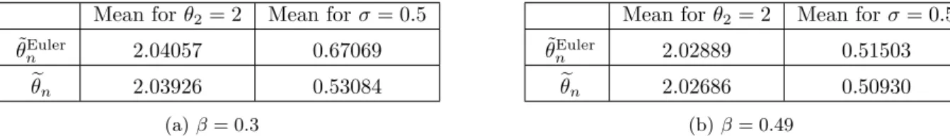
To illustrate the estimation method, we focus on the estimation of the parametersθ2 andσ2only.
For numerical simulations we choose the parameters as we did above Table 1.
The real values of the parameters we want to estimate areθ2 = 2 andσ= 0.5; we estimate the bias of
the estimators using a Monte Carlo method based on 500 replications.
We see that there is not a big difference in the estimation ofθ2with and without the correction term
while, regardingσ2, the estimator found through our approximated function ˜m and ˜m2 performs better
than the estimator we got through Euler scheme, especially forβ smaller. The two estimators ofθ2differs in fact only for the contribution of the jumps ∆J1n =
c2∆2nβ γ R Ruϕ(u)F( uc∆βn γ )du
Mean forθ2= 2 Mean forσ= 0.5 ˜ θEuler n 2.04057 0.67069 e θn 2.03926 0.53084 (a)β= 0.3
Mean forθ2= 2 Mean forσ= 0.5
˜ θEuler n 2.02889 0.51503 e θn 2.02686 0.50930 (b)β= 0.49
Table 3: Monte Carlo estimates of θ2 andσ2 from 500 samples. We have here fixed β= 0.3 in the first
table and β= 0.49 in the second one.
that is in this case close to zero, because of the natural choice of taking a truncated function which is symmetric. Indeed, even if the density functionF isn’t symmetric, asymptotically the only contribution it gives is due by its value in zero and, therefore, the symmetry ofϕis enough to ensure the limit of the integral is zero.
Also in this case the estimator θen performs well for anyβ, which means that even if we take a wrong
thresholdcfor which the well detection of the jumps is not guaranteed, the performance of the estimator
e
θn remains high.
6
Preliminary results
Before proving the main statistical results of Section 3, we need to state several propositions which will be useful in the sequel. They will be proven in Section A.1.
6.1
Limit theorems
The asymptotic properties of estimators are deduced from the asymptotic behavior of the contrast func-tion. We therefore state some propositions useful to get the asymptotic behavior of Un.
Proposition 5. Suppose that Assumptions 1 to 4 and AStep hold, ∆n →0 and Tn → ∞ and f is a
differentiable functionR×Θ→Rsuch that|f(x, θ)| ≤c(1 +|x|c),|∂xf(x, θ)| ≤c(1 +|x|c)and, forϑ=µ
and ϑ=σ,|∂ϑf(x, θ)| ≤c(1 +|x|c). Thenx7→f(x, θ) is aπ-integrable function for anyθ∈Θand the
following convergences hold as n→ ∞: 1.| 1 Tn Pn−1 i=0 ∆n,if(Xti, θ)1{|Xti|≤∆−n,ik} − R Rf(x, θ)π(dx)| P −→0, 2. | 1 Tn Pn−1 i=0 ∆n,if(Xti, θ)ϕ∆βn,i(Xti+1−Xti)1{|Xti|≤∆−k n,i} − R Rf(x, θ)π(dx)| P −→0, 3. |1 n Pn−1 i=0 f(Xti, θ)1{|Xti|≤∆−n,ik} − R Rf(x, θ)π(dx)| P −→0, 4. |1 n Pn−1 i=0 f(Xti, θ)ϕ∆βn,i(Xti+1−Xti)1{|Xti|≤∆−k n,i} − R Rf(x, θ)π(dx)| P −→0.
Statements 1−2 and 3−4 of the proposition here above, as well as the first and the second point of Proposition 6 below, turn out being similar if the sampling step ∆n,i = ∆n considered is uniform.
Otherwise, we need these two different convergences because, in order to estimate µ and σ jointly, we have to deal with different scaling of the contrast function.
Proposition 6. Suppose that Assumptions 1 to 4 and AStep hold, ∆n → 0 and Tn → ∞ and f:
R×Θ→R. Moreover we suppose that ∃c: |f(x, θ)| ≤c(1 +|x|c)and that β∈(14, 1 2). Then, ∀θ∈Θ, 1. 1 Tn n−1 X i=0 f(Xti, θ) (Xti+1−m(µ, σ, Xti)) 2ϕ ∆βn,i(Xti+1−Xti)1{|Xti|≤∆−n,ik} P −→ Z R f(x, θ)a2(x, σ0)π(dx). 2. 1 n n−1 X i=0 f(Xti, θ) ∆n,i (Xti+1−m(µ, σ, Xti)) 2ϕ ∆βn,i(Xti+1−Xti)1{|Xti|≤∆−n,ik} P −→ Z R f(x, θ)a2(x, σ0)π(dx).
The proof relies on the following lemma. In the sequel we will denoteEi[.] forE[.|Fti], where (Fs)sis
the filtration defined in Lemma 1.
Lemma 3. Suppose that Assumptions 1 to 4 hold. Moreover we suppose that β∈(14,12). Then
1.Ei[(Xti+1−m(µ, σ, Xti)) 2ϕ2 ∆βn,i(Xti+1−Xti)] = ∆n,ia 2(X ti, σ0) +R(θ,∆ 1+β n,i , Xti), (23)
2.Ei[(Xti+1−m(µ, σ, Xti)) 4ϕ4 ∆βn,i(Xti+1−Xti)] = 3∆ 2 n,ia 4(X ti, σ0) +R(θ,∆ 7 4+β n,i , Xti), (24) 3.Fork≥1, |Ei[(Xti+1−m(µ, σ, Xti))ϕ k ∆βn,i(Xti+1−Xti)]| ≤R(θ,∆n,i, Xti), (25) 4.Fork≥2,∀k0>0, Ei[|Xti+1−m(µ, σ, Xti)| k|ϕ ∆βn,i(Xti+1−Xti)| k0]≤R(θ,∆k2∧(1+βk) n,i , Xti). (26) 5.∀k0>0, Ei[(Xti+1−m(µ0, σ0, Xti)) 3 |ϕ∆β n,i (Xti+1−Xti)| k0] =R(θ 0,∆ 4 3+β n,i , Xti).
We observe that the first and the second points here above are particular cases of the the fourth one, in which we get some better estimation. In particular, we can identify in detail the main term.
Concerning the fifth point, instead, we remark that fork= 3 we don’t have the main contribution of the Brownian part anymore, which gave us the rest function of size ∆k2
n,i in (26). In this case the main term
of the development is given by the square of the Brownian integral times the jump part, which magnitude can be estimated by 43+β.
In next lemma we consider the derivatives ofϕ, getting an improvement of the estimations here above. It relies on the fact that, from the definition we gave of such a function, we know its derivatives are different from zero only if the increments of our process are smaller than 2∆βn,i (as it was forϕ) and bigger than ∆βn,i (extra bound that we did not get using ϕ). Having therefore no longer only an upper bound but also a lower bound for Xti+1−Xti, it is now possible to prove a better version of (26):
Lemma 4. Suppose that Assumptions A1-A5 A7 and Ad hold. Then ∀p≥1,∀k≥1 and∀r >0,
Ei[|Xtθi+1−m(µ, σ, Xti)| p|ϕ(k) ∆βn,i(X θ ti+1−X θ ti)| r]≤R(θ, h1+βp, X ti).
Considering only the jump part, the following result holds:
Lemma 5. Suppose that Assumptions A1-A4 holds. Then, ∀q≥1 we have
Ei[|∆XiJϕ∆βn,i(∆iX)| q] =R(θ 0,∆ (1+βq)∧q n,i , Xti), where∆XJ i := Rti+1 ti R Rzγ(Xs−)˜µ(ds, dz).
Other estimation about the expected value of the jump part in the presence of an indicator function which is 0 if the increments are bigger thanc∆βn,i are gathered in Lemma 4 of [3].
Using the lemmas stated here above, it is possible to prove the following proposition, that will be proved in Section A.1 and which is useful to show the tightness of the contrast function.
Proposition 7. Suppose that Assumptions 1 to 4 and AStep hold, ∆n → 0 and Tn → ∞ and gi,n is
a differentiable function R×Θ → R such that |gi,n(x, θ)| ≤ c(1 +|x|c) and, for ϑ = µ and ϑ = σ,
|∂ϑgi,n(x, θ)| ≤c(1 +|x|c). We define Sn(θ) := 1 Tn n−1 X i=0 (Xti+1−m(µ, σ, Xti))ϕ∆βn,i(Xti+1−Xti)gi,n(Xti, θ). ThenSn(θ)is tight in (C(Θ),k.k∞).
6.2
Derivatives of
m
and
m
2We now state some propositions which concern the derivatives of m and m2 that will be useful in the
sequel.
Proposition 8. Suppose that Assumptions A1-A5 A7 and Ad hold. Then, for|x| ≤∆−k0
n,i and∀ > 0, we have 1. ∂µm(µ, σ, Xti) = ∆n,i∂µb(Xti, µ) +R(θ,∆ 5 2−β− n,i , Xti), 2.|∂σm(µ, σ, Xti)| ≤R(θ,∆n,i, Xti), 3.|∂µm2(µ, σ, Xti)| ≤R(θ,∆ 2 n,i, Xti), 4. ∂σm2(µ, σ, Xti) = 2∆n,i∂σa(Xti, σ)a(Xti, σ) +R(θ,∆ 1+β n,i , Xti).
Estimation on the second derivatives are gathered in the following proposition:
Proposition 9. Suppose that Assumptions A1 - A5, A7 and Ad hold. Then
|∂µσ2 m(µ, σ, Xti)| ≤R(θ,∆ 3 2 n,i, Xti), |∂ 2 σm(µ, σ, Xti)| ≤R(θ,∆n,i, Xti), (27) ∂µ2m(µ, σ, Xti) = ∆n,i∂ 2 µb(µ, Xti) +R(θ,∆ 3 2 n,i, Xti), (28) |∂µσ2 m2(µ, σ, Xti)| ≤R(θ,∆ 2 n,i, Xti), |∂ 2 µm2(µ, σ, Xti)| ≤R(θ,∆ 2 n,i, Xti), (29) ∂σ2m2(µ, σ, Xti) = 2∆n,i∂σa(σ, Xti)a(σ, Xti) +R(θ,∆ 3 2 n,i, Xti). (30)
Deriving once again, the orders do not get worse. Indeed, the following estimations hold.
Proposition 10. Suppose that Assumptions A1 - A5, A7 and Ad hold. Then
1. |∂µ3m2(µ, σ, Xti)| ≤R(θ,∆ 2 n,i, Xti); 2. |∂ 3 σµσm2(µ, σ, Xti)| ≤R(θ,∆ 2 n,i, Xti), 3. |∂µµσ3 m2(µ, σ, Xti)| ≤R(θ,∆ 2 n,i, Xti); 4. |∂ 3 σm2(µ, σ, Xti)| ≤R(θ,∆n,i, Xti), 5. |∂µ3m(µ, σ, Xti)| ≤R(θ,∆n,i, Xti); 6. |∂ 3 σµσm(µ, σ, Xti)| ≤R(θ,∆ 3 2 n,i, Xti), 7. |∂µµσ3 m(µ, σ, Xti)| ≤R(θ,∆ 3 2 n,i, Xti); 8. |∂ 3 σm(µ, σ, Xti)| ≤R(θ,∆n,i, Xti).
Propositions 8, 9 and 10 will be proved in the appendix.
7
Proof of main results
We first of all study the asymptotic behaviour of the contrast, from which we find the consistency of our estimator.
We underline that, to get the consistency of the drift parameter, the normalization of the contrast function is different than the normalization we use to find the consistency of ˆσn. Even if it doesn’t seem a natural
choice, it works well on the basis of Proposition 6.
7.1
Contrast’s convergence
To prove the contrast convergences, the development (10) ofm2will be useful. We have shown in [2] (see
(16) also) that under Assumptions (A1)-(A4) the following development ofm(µ, σ, x) holds :
m(µ, σ, x) =x+ ∆n,ib(x, µ) +RJ(∆n,i, x) +r1(µ, σ, x), (31)
wherer1(µ, σ, x) is a particularR(θ,∆n,i1+δ, Xti) function (withδ >0) andR
J(∆
n,i, x) =−∆n,iRRzγ(x)[1−
ϕ∆β
n,i(γ(x)z)]F(z)dz; theJ underlines that it turns out from a jump term. It has the same properties of
the function R defined in Section 4.2 but it does not depend onθ.
Let us now prove the consistency of ˆθn. The first step are the following lemmas:
Lemma 6. Suppose that A1 - A5,AStep and Ad hold. Moreover we suppose that β∈(14,12). Then
1 nUn(µ, σ) P −→ Z R [c(x, σ0) c(x, σ) +log(c(x, σ))]π(dx), (32)
wherec(x, σ) =a2(x, σ) andπis the invariant distribution defined in Lemma 2.
Lemma 6 is useful to prove the consistency of ˆσn, while we will use next lemma to show the consistency
of ˆµn
Lemma 7. Suppose that A1 - A5, AStep and Ad hold. Moreover we suppose that β ∈(1 4, 1 2) and that 2δ1>1. Then 1 Tn (Un(µ, σ)−Un(µ0, σ))−→P Z R (b(x, µ0)−b(x, µ))2 c(x, σ) π(dx) + Z R [r(µ, σ, x)−r(µ0, σ, x)](1− c(x, σ0) c(x, σ))π(dx), (33)
7.1.1 Proof of Lemma 6
Proof. We first of all observe that by the equation (10) we have, for|Xti| ≤∆ −k n,i, 1 m2(µ, σ, Xti) = 1 ∆n,ic(Xti, σ)(1 + ∆ δ1 n,i r(Xti) c(Xti,σ)+ ∆n,ir(µ, σ, Xti) +R(θ,∆ 1+δ2 n,i , Xti)) = = 1 ∆n,ic(Xti, σ) (1−∆δ1 n,i r(Xti) c(Xti, σ) −∆n,ir(µ, σ, Xti) +R(θ,∆ 2δ1∧(1+δ2)∧2 n,i , Xti)). (34)
In the sequel we will just write ¯rfor 2δ1∧(1+δ2)∧2. We observe that, as a consequence of the Assumption
Ad, we have for bothϑ=µandϑ=σ,|∂ϑR(θ,∆rn,i¯ , Xti)| ≤R(θ,∆
¯
r
n,i, Xti), where the two rest functions
are not necessarily the same. Similarly, log(m2(µ, σ, Xti) ∆n,i ) =log(c(Xti, σ)) +log(1 + ∆ δ1 n,i r(Xti) c(Xti, σ) + ∆n,ir(µ, σ, Xti) +R(θ,∆ 1+δ2 n,i , Xti)) = =log(c(Xti, σ)) + ∆ δ1 n,i r(Xti) c(Xti, σ) + ∆n,ir(µ, σ, Xti) +R(θ,∆ ¯ r n,i, Xti). (35)
Using both (34) and (35) in the definition ofUn(µ, σ), we have to show that
1 n n−1 X i=0 (Xti+1−m(µ, σ, Xti)) 2 ∆n,ic(Xti, σ) ϕ∆β n,i (Xti+1−Xti)1{|Xti|≤∆−n,ik}(1−∆ δ1 n,i r(Xti) c(Xti, σ) −∆n,ir(µ, σ, Xti)+R(θ,∆ ¯ r n,i, Xti))+ +1 n n−1 X i=0 (log(c(Xti, σ))+∆ δ1 n,i r(Xti) c(Xti, σ) +∆n,ir(µ, σ, Xti)+R(θ,∆ ¯ r n,i, Xti))ϕ∆βn,i(Xti+1−Xti)1{|Xti|≤∆−k n,i} =: 8 X j=1 Ijn
converges to the right hand side of (32). We know thatIn
1 P −→R R( c(x,σ0) c(x,σ))π(dx) because of Proposition 6.
Using the third point of Proposition 5, In
5
P −→R
Rlog(c(x, σ))π(dx). All the other terms converge to zero
in norm 1 and so in probability. Indeed, passing through the conditional expectation and using the first point of Lemma 3 we have
E[|I2n|]≤ 1 n n−1 X i=0 E[| ∆δ1 n,ir(Xti) ∆n,ic2(Xti, σ) Ei[(Xti+1−m(µ, σ, Xti)) 2ϕ ∆βn,i(Xti+1−Xti)]1{|Xti|≤∆−k n,i}| ]≤ ≤ ∆ δ1 n n n−1 X i=0 E[|R(θ,1, Xti)|]≤c∆ δ1 n,
reminding thatr(Xti) is a functionR(θ,1, Xti) by its definition and having used the property (9) on R,
its polynomial growth and the third point of Lemma 2. In the same way we obtain
E[|I3n|]≤c∆n and E[|I4n|]≤c∆ ¯
r n,
that goes to zero since ¯r= 2δ1∧(1 +δ2)∧2 is always positive.
ConcerningI6n, as a consequence of the definition of r(x) and the fact that ∆n,i≤∆n we have again
E[|I6n|]≤ ∆δ1 n n n−1 X i=0 E[|R(θ,1, Xti)|]≤c∆ δ1 n,
which converges to zero for n→ ∞. Again, acting in the same way we have
E[|I7n|]≤c∆n and E[|I8n|]≤c∆ ¯ r n. Convergence (32) follows. 7.1.2 Proof of Lemma 7
Proof. Using again (34) and (35) we have that 1 Tn (Un(µ, σ)−Un(µ0, σ)) = 1 Tn n−1 X i=0 [(Xti+1−m(µ, σ, Xti)) 2 ∆n,ic(Xti, σ) −(Xti+1−m(µ0, σ, Xti)) 2 ∆n,ic(Xti, σ) ]ϕ∆β n,i(∆iX)1{|Xti|≤∆−n,ik}+
+ 1 Tn n−1 X i=0 ∆δ1 n,i r(Xti) c(Xti, σ) [(Xti+1−m(µ, σ, Xti)) 2 ∆n,ic(Xti, σ) −(Xti+1−m(µ0, σ, Xti)) 2 ∆n,ic(Xti, σ) ]ϕ∆β n,i (∆iX)1{|X ti|≤∆−n,ik}+ + 1 Tn n−1 X i=0 ∆n,ir(µ, σ, Xti)[1− (Xti+1−m(µ, σ, Xti)) 2 ∆n,ic(Xti, σ) ]ϕ∆β n,i (∆iX)1{|Xti|≤∆−k n,i} + − 1 Tn n−1 X i=0 ∆n,ir(µ0, σ, Xti)[1− (Xti+1−m(µ0, σ, Xti)) 2 ∆n,ic(Xti, σ) ]ϕ∆β n,i (∆iX)1{|X ti|≤∆−n,ik}+ + 1 Tn n−1 X i=0 [R((µ, σ),∆rn,i¯ , Xti) +R((µ, σ),∆ ¯ r n,i, Xti) (Xti+1−m(µ, σ, Xti)) 2 ∆n,ic(Xti, σ) ]ϕ∆β n,i (∆iX)1{|Xti|≤∆−k n,i} + + 1 Tn n−1 X i=0 [R((µ0, σ),∆rn,i¯ , Xti)+R((µ0, σ),∆ ¯ r n,i, Xti) (Xti+1−m(µ0, σ, Xti)) 2 ∆n,ic(Xti, σ) ]ϕ∆β n,i (∆iX)1{|X ti|≤∆−n,ik}=: 6 X j=1 Ijn,
where we have introduced the notation ∆iX:=Xti+1−Xti and we recall that ¯r= 2δ1∧(1 +δ2)∧2.
We have already proved in Lemma 4 of [2] thatIn
1 P −→R R (b(x,µ0)−b(x,µ))2 c(x,σ) π(dx). We observe thatI n 2 differs from In
1 only from the presence of ∆
δ1
n,i r(Xti)
c(Xti,σ) and so, sinceδ1 is positive, acting exactly as we did in
order to prove the convergence ofIn
1 it is possible to show that the added ∆
δ1 n,imakeI n 2 converge to zero in probability. ConcerningIn 3, 1 Tn n−1 X i=0 ∆n,ir(µ, σ, Xti)ϕ∆βn,i(∆iX)1{|Xti|≤∆−k n,i} P −→ Z R r(µ, σ, x)π(dx) (36)
as a consequence of the second point of Proposition 5. Moreover, using the third point of Proposition 6, we have that 1 Tn n−1 X i=0 ∆n,ir(µ, σ, Xti) (Xti+1−m(µ, σ, Xti)) 2 ∆n,ic(Xti, σ) ϕ∆β n,i(∆iX)1{|Xti|≤∆−n,ik} P −→ Z R r(µ, σ, x)c(x, σ0) c(x, σ)π(dx). (37) From (36) and (37) it follows
I3n−→P
Z
R
r(µ, σ, x)[1−c(x, σ0)
c(x, σ)]π(dx). Acting on I4n exactly like we did on I3n we get
I4n−→P Z R r(µ0, σ, x)[1− c(x, σ0) c(x, σ)]π(dx). ConcerningI5n, it is 1 Tn n−1 X i=0
R(θ,∆rn,i¯ , Xti)ϕ∆βn,i(∆iX)1{|Xti|≤∆−n,ik} ≤∆ ¯ r−1 n 1 n n−1 X i=0 R(θ,1, Xti)ϕ∆βn,i(∆iX),
which converges to zero in norm 1 and so in probability because of the boundedness ofϕ, the polynomial growth ofR, the fact that T1
n =O(
1
n∆n) and thatr−1 is always positive since we have assumed 2δ1>1.
Moreover, passing through the conditional expectation and using the first point of Lemma 3 we have that 1 Tn n−1 X i=0 E[R(θ,∆rn,i¯ , Xti)Ei[ (Xti+1−m(µ, σ, Xti)) 2 ∆n,ic(Xti, σ) ϕ∆β n,i (∆iX)]1{|X ti|≤∆−n,ik}]≤∆ ¯ r−1 n 1 n n−1 X i=0 E[R(θ,1, Xti)]≤c∆ ¯ r−1 n .
We have therefore proved that the second part ofI5nconverges to 0 in norm 1 and therefore in probability. It follows In
5
P
−→0 and, acting exactly in the same way, we have alsoIn
6
P
7.2
Consistency of the estimator.
In order to prove the consistency of ˆθn, we need that the convergences (32) and (33) take place in
proba-bility uniformly in both the parameters, we want therefore to show the uniformity of the convergence in θ.
We regard Un(µ,σ)
n and Sn(µ, σ) :=
1
Tn(Un(µ, σ)−Un(µ0, σ)) as random elements taking values in
(C(Θ),k.k∞). It suffices to prove the tightness of these sequences; to do it we need some estimations for the derivatives ofmandm2with respect to both the parameters, which are stated in Proposition 8, that
will be proved in the Appendix. Such a proposition will be also useful to study the asymptotic behavior of the derivatives of the contrast function. We observe that, as a consequence of (31) and Proposition 8, forϑ=µorϑ=σit is|∂ϑr1(µ, σ, x)| ≤R(θ,∆n,i, Xti).
Lemma 8. Suppose that Assumption A1-A5, Ad,AStep and A7 are satisfied. Then, the sequence Un(µ,σ)
n
is tight in (C(Θ),k.k∞).
Proof. The tightness is implied by supn 1
nE[supµ,σ|∂ϑUn(µ, σ)|]<∞(see Corollary B.1 in [26]), forϑ=µ
andϑ=σ. It is ∂ϑUn(µ, σ) = n−1 X i=0 [−2∂ϑm(µ, σ, Xti)(Xti+1−m(µ, σ, Xti)) m2(µ, σ, Xti) −∂ϑm2(µ, σ, Xti)(Xti+1−m(µ, σ, Xti)) 2 m2 2(µ, σ, Xti) + (38) +∂ϑm2(µ, σ, Xti) m2(µ, σ, Xti) ]ϕ∆β n,i (∆iX)]1{|X ti|≤∆−n,ik}.
Using the first and the third point of Proposition 8 and the development (10) ofm2 it follows
E[sup µ,σ |∂µUn(µ, σ)|]≤ n−1 X i=0 E[sup µ,σ |R(θ,1, Xti)(Xti+1−m(µ, σ, Xti))ϕ∆βn,i(∆iX)|1i,n]+ + n−1 X i=0 E[sup µ,σ |R(θ,1, Xti)(Xti+1−m(µ, σ, Xti)) 2ϕ ∆βn,i(∆iX)|1i,n] + n−1 X i=0 E[sup µ,σ |R(θ,∆n,i, Xti)|1i,n], (39)
where we have used 1i,ninstead of 1{|X
ti|≤∆−n,ik}
to shorten the notation. We observe that E[sup µ,σ |R(θ,1, Xti)(Xti+1−m(µ, σ, Xti))ϕ∆βn,i(∆iX)|1i,n]≤ ≤E[(sup µ,σ |R(θ,1, Xti)|)(sup µ,σ |(Xti+1−m(µ, σ, Xti))ϕ∆βn,i(∆iX)|)1i,n]≤ ≤E[(sup µ,σ |R(θ,1, Xti)|1i,n)(|(Xti+1−m(µ0, σ, Xti))ϕ∆βn,i(∆iX)|)]+ +cE[(sup µ,σ |R(θ,1, Xti)|)(sup µ,σ |m(µ, σ, Xti)−m(µ0, σ, Xti))|)1i,n]. (40)
We can now use Cauchy-Schwartz inequality and (23) in Lemma 3 on the first, while on the second we use the development (31) ofmgetting that (40) is upper bounded by
cE[R(θ,∆n,i, Xti)] 1 2+cE[(sup µ,σ |R(θ,1, Xti)|)(sup µ,σ |∆n,i(b(Xti, µ)−b(Xti, µ0))+r1(µ, σ, Xti)−r1(µ0, σ, Xti)|)]≤ ≤c∆ 1 2 n+cE[sup µ,σ |R(θ,∆n,i, Xti)|]≤c∆ 1 2 n +c∆n ≤c∆ 1 2 n, (41)
where we have also used the boundedness of ϕ, the fact that R has polynomial growth uniformly in θ and the third point of Lemma 2 to say that our process has finite moments.
In the same way,
E[sup
µ,σ
|R(θ,1, Xti)(Xti+1−m(µ, σ, Xti))
2
ϕ∆β
n,i(∆iX)|1i,n]≤E[supµ,σ|R(θ,∆n,i, Xti)|]+E[supµ,σ|R(θ,∆
2
n,i, Xti)|]≤c∆n.
(42) Replacing (41) and (42) in (39) it follows
sup n 1 nE[supµ,σ |∂µUn(µ, σ)|]≤c∆ 1 2 n ≤c <∞.
We can act in the same way on ∂σUn(µ, σ). Considering this time the second and the fourth point of
Proposition 8 and still using the development (10) of m2and (23) in Lemma 3 it follows
sup n 1 nE[supµ,σ |∂σUn(µ, σ)|]≤sup n 1 n n−1 X i=0 E[sup µ,σ |R(θ,∆ 1 2 n,i, Xti) +R(θ,1, Xti)|]≤c <∞.
The tightness is therefore proved.
Lemma 9. Suppose that Assumption A1-A5, A7,AStep and Ad are satisfied. We suppose moreover that δ1 in the Assumption Ad is such that 2δ1 >1. Then, the sequenceSn(µ, σ) = T1
n(Un(µ, σ)−Un(µ0, σ))
is tight in (C(Θ),k.k∞).
Proof. Let’s take again the notation used in the proof of Lemma 7, for whichSn(µ, σ) =P6j=1Ijn. Since
the sum of tight sequences is still tight, we will proceed showing that they are all tight. We start with I3n; acting as we did in Lemma 8, we prove that supnE[supµ,σ|∂ϑI3n|]<∞. We observe that, forϑ=µ
andϑ=σ, ∂ϑI3n= 1 Tn n−1 X i=0 ∆n,i[∂ϑr(µ, σ, Xti)(1− (Xti+1−m(µ, σ, Xti)) 2 ∆n,ic(Xti, σ) )+ −r(µ, σ, Xti)∂ϑ( (Xti+1−m(µ, σ, Xti)) 2 ∆n,ic(Xti, σ) )]ϕ∆β n,i(∆iX)1{|Xti|≤∆−n,ik}=:I n 3,1+I3n,2.
OnI3n,1we use the first point of Lemma 3 and that|∂ϑr(µ, σ, Xti)| ≤R(θ,1, Xti) as stated in Assumption
Ad to get sup n E [sup µ,σ |I3n,1|]≤c+ sup n 1 n∆n n−1 X i=0 E[Ei[sup µ,σ |R(θ,1, Xti)(Xti+1−m(µ, σ, Xti)) 2ϕ ∆βn,i(∆iX)|1i,n]]≤c (43) where we have used the polynomial growth of R, the third point of Lemma 2 and (42) and the notation 1i,n instead of 1{|X
ti|≤∆−n,ik}.
Concerning In
3,2, the derivatives of
(Xti+1−m(µ,σ,Xti))2
∆n,ic(Xti,σ) with respect toµ andσ are different but in both
cases they are upper bounded, using the first and the second point of Proposition 8, by|R(θ,1, Xti)(Xti+1− m(µ, σ, Xti))ϕ∆βn,i(∆iX)|. We can therefore use (40) and (41), getting
sup n E [sup µ,σ |I3n,2|]≤csup n ∆ 1 2 n ≤c <∞. (44)
From (43) and (44) it follows the tightness of I3n. Acting exactly in the same way onI4n it is clear it is tight too. ConcerningI5n andI6n, recalling that the functionR(θ,∆rn,i¯ , Xti) turns out from (34) and it is
such that its derivatives with respect to both the parameters remains of the same order, we observe it is possible to act like we did on I3n getting
sup n E [sup µ,σ |I5n|]≤c∆n¯r−1+c∆¯r−12 n <∞,
since we have chosen 2δ1>1 and so ¯r−1 is positive. Clearly the same estimation hold forI6n.
We now prove that In
1 is tight. To do it we observe that, using the development (31) and the dynamic
(3) of the processX we have
Xti+1−m(µ, σ, Xti) = Z ti+1 ti b(Xs, µ0)ds+ Z ti+1 ti a(σ0, Xs)dWs+ Z ti+1 ti Z R\{0} γ(Xs−)zµ˜(ds, dz)+ (45) −RJ(∆n,i, Xti)−∆n,ib(Xti, µ)−r1(µ, σ, Xti).
It is worth noting that only the last two terms here above depend onµand so replacing (45) inI1n some
terms are deleted by compensation. Therefore we can define
I1n,1:= 1 Tn n−1 X i=0 ϕ∆β n,i (∆iX)1{|X ti|≤∆−n,ik} ∆n,ic(σ, Xti) [∆2n,i(b2(Xti, µ)−b 2(X ti, µ0)) +r 2 1(µ, σ, Xti)−r 2 1(µ0, σ, Xti)+ +2∆n,ib(Xti, µ)r1(µ, σ, Xti)−2∆n,ib(Xti, µ0)r1(µ0, σ, Xti) + 2[ Z ti+1 ti b(Xs, µ0)ds+ ∆XiJ+