1 INTRODUCTION
An aircraft fuel system is a complex system, con-sisting of a large number of different components that can fail, sometimes in more than one failure mode. In addition, the failure modes will have an effect on the performance of the system, at different degrees of se-verity. In order to be able to monitor system perfor-mance and detect early signs of failure, sensors are used on the system, such as flow, pressure and level sensors on the fuel system. In addition, if a compo-nent failure can be diagnosed, appropriate actions can be taken in flight, such as abort or adapt the mission, and maintenance work can be carried out on the ground on the part of the system with the failure.
However, sensors themselves have associated costs, such as purchase, installation and the mainte-nance cost, and their weight needs to be considered. Therefore, a correct balance between the number of sensors, their positioning on the system and the infor-mation provided about the faults needs to be achieved.
In order to be able to propose a sensor selection method, a sensor performance metric is defined in this paper. This metric considers the features of each in-dividual sensor and their groups, such as the number of faults that can be detected and the number of com-ponent failures that can be diagnosed. The compo-nent failures in the system can be diagnosed using a Bayesian Belief Network (BBN). The evidence from
sensor readings can be introduced to the network, up-dating the probability of the system components be-ing in the failed state, therefore, indicatbe-ing the com-ponents that are most likely to have failed.
In this paper, a brief overview of the previous re-search is given in section 2, followed by outlining an example system in section 3. Section 4 introduces the sensor performance metric and the methodology for fault diagnostics. Section 5 shows the application of the method to the example system and section 6 anal-yses the application of the methodology. Finally, sec-tion 7 summarises the work presented in this paper and suggests future work.
2 PREVIOUS RESEARCH
In this section, some published work on sensor se-lection strategies is discussed, which is followed by work on system modelling and fault diagnostics. 2.1 Sensor selection
A range of approaches for determining which sen-sor combination is best have been developed. For ex-ample, Maul et al. (2008) developed a performance metric for aircraft systems. The authors demonstrated their work with an example system, which was a sub-system of a space shuttle main engine. This method requires human input for model parameters and as a
A sensor selection method for fault diagnostics
J. Reeves, R. Remenyte-Prescott, J. Andrews
Resilience Engineering Research Group, University Of Nottingham, University Park, Nottingham, NG7 2RD, UK
ABSTRACT: In the modern world, systems are becoming increasingly complex, consisting of large numbers of components and their failures. In order to monitor system performance and to detect faults and diagnose failures, sensors can be used. However, using sensors can increase the cost and weight of the system. Therefore, sensors need to be selected based on the information that they provide.
result, the selection process is subjective. Pourali & Mosleh (2012) developed a utility function, but this work does not consider the ability to diagnose fail-ures. Lambert & Farrington (2007) used a cost-bene-fit function, outlining the best locations for sensors to detect chemical, biological and radiological air con-taminants. However, this function uses multiple case specific factors such as the density of elderly people, making it difficult to apply the method to other types of systems.
A number of authors, such as Santi et al. (2005), Spanache et al. (2004), and Maul et al. (2008), used genetic algorithms to optimise the sensor selection process for various systems, such as aircraft/space-crafts and a benchmark actuator.
2.2 System modelling and fault diagnostics
One of the most commonly used model-based fault diagnostics technique is fault tree analysis, also used for system reliability assessment. Hurdle et al. (2008) modelled a simple water tank system, using non-co-herent fault trees, which consider NOT logic in order to more accurately model the system. In Hurdle et al. (2007), the technique has been extended to model an aircraft fuel system. The authors consider multiple system operation phases, known as a phased mission, and they introduce a sensor effectiveness index that considers which failures are diagnosed by the sensors. In Equation 1, the effectiveness index, IE, is given,
where N is the number of sensor patterns observed, ni
is the number of failures identified, nci is the number
of patterns observed that gives the correct causes, and
nai is the number of potential causes that exist.
IE= 1 N∑ (
nci ni) (
nci nai) N
i=1
(1)
However, an individual fault tree is required to be developed for each possible set of symptoms.
Bartlett et al. (2006) use an alternative method of digraphs, to diagnose failures in the aircraft fuel sys-tem. The authors compare the two approaches and they state that the fault tree method determines the combinations of component failures that can cause different sensor readings, whereas the digraph method enables the propagation of the failure through the system. Digraphs are also limited by the require-ment to classify the strength of the relationship be-tween events in the network. This introduces subjec-tivity into the modelling. The authors suggest that the two techniques complement each other, so they should be used together.
Another alternative fault diagnostics method, Petri Nets, was proposed by Lloyd et al. (2014), where faults on an aircraft fuel rig can be confirmed as true or cancelled as false, and the method can be applied
to reducing the number of false fault alarms on air-craft fuel systems.
The fault diagnostics technique used in this paper is the BBN. BBNs are directed acyclic graphs and the state of each node is determined using conditional probability tables (CPTs). The BBNs can be built us-ing fault trees, as suggested by Lampis & Andrews (2013). Evidence about a fault can be introduced in the BBN directly, and the probability of each compo-nent failure mode occurrence is calculated, which ranks the causes of that fault. This feature was the main reason for selecting the BBN as the fault diag-nostic method used in this paper, for demonstrating the effectiveness of the selected sensors.
3 SYSTEM DESCRIPTION
In this section, an example system is introduced, which is used to demonstrate the proposed methodol-ogy.
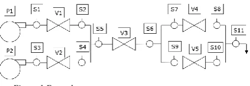
The system in Figure 1 consists of 5 valves (V1, V2, V3, V4 and V5), and 2 pumps (P1 and P2). The flow is from left to right, where it exits the system via a drain. Sensors S1 – S10 are positioned either side of each of the valves and sensor S11 is positioned be-fore the drain. Ns is the number of possible sensors,
Ns = 11 for this example system.
Under normal operating conditions, each of the pumps, P1 and P2, supply a quantity of fuel to the system, which passes through valve V1 and V2 re-spectively. Then the fuel from the two parallel lines passes through valve V3, before going through the next two parallel lines with valves V4 and V5 at the same rate. Finally, the fuel leaves the system through the drain. It is assumed that the flow rate through the parallel lines is half of the flow rate through the cen-tral part of the system.
Each component can be in one of two states: work-ing or failed. The pumps are workwork-ing when they are supplying fuel to the system, and the valves are work-ing when they are allowwork-ing fuel to pass through the system. No partial failures are considered in this pa-per, such as partial supply of fuel or partially blocked valves.
[image:2.595.309.563.415.503.2]No more than two component failures occurring at the same time are considered, for example, P1 fails and the rest of the components work, or P1 and V1
fails and the rest of the components work. Combina-tions of 3 or more failures are not considered due to a very low probability of such event occurrence. In the proposed methodology, 1 or 2 component failures are defined as considered failures. Note that there is no time delay between the occurrences of two failures.
A component failure can be critical to the perfor-mance of the system, even cause system failure. For this example system, system failure is defined as a failure that results in a reduction of the fuel exiting through the drain. This will occur when at least one of the pumps cannot supply fuel to the drain by a pump being off, or at least one valve is blocked, de-pending on its location. The minimal cut sets for this system failure logic are: {P1}, {P2}, {V1}, {V2}, {V3} and {V4, V5}. Note that if valve V4 or valve V5 (but not both) is blocked, there is no reduction in the supply of fuel from the pumps, all the fuel can pass through the other parallel line to the one with the failed valve and system failure does not occur.
In the next section, the methodologies for sensor selection, system modelling and fault diagnostics are introduced.
4 PROPOSED METHODOLOGY FOR SENSOR
SELECTION AND FAULT DIAGNOSTICS There are three parts of the proposed methodol-ogy: the sensor selection, the system modelling and the fault diagnostics. Firstly, the sensors to be used in the system are selected. The system can then be modelled with these sensors included in the system. The model obtained can then be used to demonstrate the effectiveness of fault diagnostics using the se-lected sensors.
4.1 Performance metric methodology for sensor selection
In order to select the sensors, a sensor performance metric is proposed in this paper, which considers the occurrence probability of the failures that can be de-tected, the ease of diagnostics of the failures, and the effect that the diagnosed failures have on system fail-ure. Note that the fault detection process is about ing able to distinguish between the normal system be-haviour (without failures) and abnormal system behaviour (with failures), whereas the fault diagnos-tics process localises the cause of the faults.
The performance metric is defined to be between 0 and 1, where 1 is the best performance value for the sensors. Note, in the equations for the performance metric discussed in the following sections, sensor s
refers to a single sensor or a group of sensors.
4.1.1 Detection Term
In order for a sensor to detect a failure, the sensor reading must deviate from the sensor reading, ex-pected for the normal system behaviour. Note, for a group of sensors, at least one of the sensors needs to have a deviated sensor reading for a failure to be de-tected.
The detection term, DE{s}, is equal to the ratio
be-tween the probability of occurrence of the detected failures and the considered failures in the system. This term is given in Equation 2, where Pd is the sum
of probabilities of considered failures occurrence that sensor s can detect, and Pmd is the sum of probabilities
of considered failures occurrence that can be detected by at least one sensor out of all possible sensors. Note, there can be hidden failures that none of the sensors can detect. Also, DE{s} is equal to 1 when
sensor s can detect all the considered failures that can be detected, and is equal to 0 when no failures can be detected by sensor s.
DE{s} = Pd
Pmd (2)
4.1.2 Diagnostic Term
The diagnostic term considers the ease of diagnos-ing which failure has occurred. For this term to be its maximum value, 1, the sensor would produce a unique sensor reading for each combination of ponent failures. Note, that the combination of com-ponent failures can also be a single comcom-ponent fail-ure. However, in reality, multiple component failure combinations can result in the same sensor reading, therefore, the diagnostic term is usually lower than 1. The term is close to 0 when there are many different component failure combinations that have similar probabilities and produce the same sensor reading.
The diagnostic term, DI{s}, consists of terms for
each of the produced deviated sensor reading combi-nations, as shown in Equation 3. Psri is the probability
that a deviated reading i of sensor s occurs. For each combination of sensor readings, multiple different combinations of component failures can be the cause. For each of these sensor readings, there will be a com-bination of component failures that will be the most likely to be the cause of the deviated sensor reading being recorded. Pmli is the probability of the most
likely combination of component failures that can cause the reading i of sensor s. These terms are summed over the number of different deviated read-ings of sensor s, nrs.
Therefore, DI{s} is the probability that the
diag-nosed failure using sensor s is the actual failure on the system.
DI{s} =
∑nrsi=1Pmli
4.1.3 Criticality Term
Finally, the criticality term considers the effects on the system by the component failures that can be de-tected by the sensors on the system.
The criticality term of the performance metric is based on the Fussell-Vesely importance measure, Cheok et al. (1998). This importance measure is se-lected over other importance measures because it can be translated to sensors with ease, adapting the defi-nition of individual components as it was originally proposed for. Other importance measures, such as Birnbaum’s importance measure were also consid-ered but the definition could not be adapted as easily, especially for combinations of sensors.
The Fussell-Vesely importance measure indicates the components contribution to system unavailability. It is calculated by subtracting the probability that sys-tem failure occurs when component j is working from the probability of system failure and normalised by the probability of system failure.
For this definition to be applied to sensors, the sub-tracted term is modified to be the probability of sys-tem failure, given that the non-deviated reading of sensor s occurs.
The criticality term, CR{s}, is given in Equation 4.
In this equation, Qsys is the system failure probability,
in other words the probability that the system fails with no knowledge of any of the component states, and Qsys(qs = 0) is the probability of system failure
given that the non-deviated reading of sensor s oc-curs.
CR{𝑠} = Qsys−Qsys(q𝑠= 0)
Qsys (4)
When the sensor does not detect any of the critical component failures, CR{s} = 0, but if all critical
fail-ures can be detected by the sensor, then CR{s} = 1. In
the next section, a discussion about combining the terms to form the sensor performance metric is given. 4.1.4 Discussion
The performance metric can be calculated using the three terms. If each term is deemed to be equally important, then an average value can be used to get the performance metric.
However, if one of the terms is significantly higher than the other terms, this can make the performance metric unrepresentative of how useful the sensors are. For example, if a sensor only detects one component failure, then the diagnostic term will be 1, regardless of the failure probability of this single component, which can be very low and insignificant. This in-creases the value of the performance metric to a much higher value than would be expected for a sensor that detects a very low percentage of component failures.
Similar effects could occur if the probability of a critical failure is relatively low, in comparison to the
probability of a failure occurring. This would result in a significantly higher criticality term if the critical failures are detected, regardless of the probability of the combinations of component failures occurring. This would also result in a higher performance metric.
In most cases, it will be important to get a balance between all three terms, but in some cases, it might be preferential to favour one of the terms. Therefore, a potential solution could be to use the performance metric as the average of the three terms in order to reduce the number of sensor combinations that can be analysed, but to then consider the individual terms separately for the final sensor selection. This enables the best sensor combination for each individual situ-ation to be selected. For example, it could be imper-ative for the criticality term to be as high as possible, as long as the other two terms are not below a certain threshold. Such conditions can be satisfied, hence giving the analyst the flexibility to choose the best sensor combination for their particular application. The performance metric is shown in Equation 5.
I{s} = 1 3((
𝑃𝑑
Pmd)+(
∑nrsi=1Pmli
∑nrsPsri i=1
)
+ (Qsys- Qsys(qs = 0)
Qsys )) (5)
In the next section, the methodology for system modelling is introduced.
4.2 Fault Diagnostics model
A BBN is developed for the example system in or-der to demonstrate how the chosen sensors can be used in fault diagnostics. The BBN was constructed using the software, “HUGIN Researcher”.
system. For a complex system, there might be a num-ber of intermediate steps applied. Finally, nodes for the sensors are included. These determine the sensor readings for different system states.
Once the BBN is built in order to diagnose com-ponent failures in the system, sensor readings are in-troduced in the BBN as evidence. The probability of the components being in each of their states is then calculated. If the failure identified by the BBN is not the actual failed component, then further evidence can be introduced until the correct component failure is identified.
The results of the fault diagnostic process can be used for prioritising maintenance or for reconfiguring the system operation due to the identified failures.
In the next section, the methodology is applied to the simple system introduced in section 3.
5 APPLICATION OF THE METHODOLOGY For illustration, it is assumed that the probability of each component failure is 0.05, such as P(A) =
0.05. Therefore, the probability that one component is failed is represented as P(A) (1 – P(A))6, and the
probability that two components are failed is repre-sented by P(A)2(1 – P(A))5.
5.1 Sensor Selection
The best possible performance metric was calcu-lated by using all eleven sensors on the system, which was equal to 0.8961: with a detection term of 1, a di-agnostics term of 0.6883 and a criticality term of 1. This means that all considered combinations of com-ponent failures can be detected (as DE{s} = 1) and
therefore all critical failures can be detected (CR{s} =
1). However, it does suggest that not all component failures can be diagnosed correctly as the value of
DI{s}is less than 1.
5.1.1 Results
Only combinations of four or less sensors are con-sidered further, as the best possible performance met-ric (0.8961) was achieved by combinations of four sensors. These combinations of sensors are:
S1 S2 S3 S7
S1 S2 S3 S9
S1 S3 S4 S7
S1 S3 S4 S9
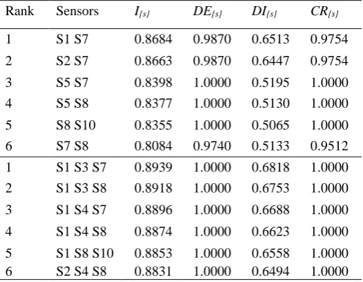
[image:5.595.305.567.56.245.2]In Table 1, individual sensor rankings are given, and in Table 2, the highest 6 rankings of combinations of 2 and 3 sensors are given. Only one combination for each ranking in Table 2 is included for brevity. There are multiple combinations of sensors with the same ranking due to the symmetry between the paral-lel lines in the system.
Table 1 Ranking of individual sensors for the system
Rank Sensor I{s} DE{s} DI{s} CR{s}
1 S7 0.8062 0.9740 0.5067 0.9512 S8 0.8062 0.9740 0.5067 0.9512 S9 0.8062 0.9740 0.5067 0.9512 S10 0.8062 0.9740 0.5067 0.9512 2 S5 0.6688 0.7532 0.3362 1.0000 S6 0.6688 0.7532 0.3362 1.0000 3 S11 0.6667 0.7532 0.3276 1.0000 4 S1 0.3901 0.4740 0.2740 0.5665 S2 0.3901 0.4740 0.2740 0.5665 S3 0.3901 0.4740 0.2740 0.5665 S4 0.3901 0.4740 0.2740 0.5665
Table 2 Ranking of combinations of 2 and 3 sensors for the system
Rank Sensors I{s} DE{s} DI{s} CR{s}
1 S1 S7 0.8684 0.9870 0.6513 0.9754 2 S2 S7 0.8663 0.9870 0.6447 0.9754 3 S5 S7 0.8398 1.0000 0.5195 1.0000 4 S5 S8 0.8377 1.0000 0.5130 1.0000 5 S8 S10 0.8355 1.0000 0.5065 1.0000 6 S7 S8 0.8084 0.9740 0.5133 0.9512 1 S1 S3 S7 0.8939 1.0000 0.6818 1.0000 2 S1 S3 S8 0.8918 1.0000 0.6753 1.0000 3 S1 S4 S7 0.8896 1.0000 0.6688 1.0000 4 S1 S4 S8 0.8874 1.0000 0.6623 1.0000 5 S1 S8 S10 0.8853 1.0000 0.6558 1.0000 6 S2 S4 S8 0.8831 1.0000 0.6494 1.0000
Further combinations of 4 sensors are not consid-ered in this paper due to the small increase in perfor-mance metric in comparison to the best combination of 3 sensors and because of the number of combina-tions of sensors (double the number of combinacombina-tions of 3 sensors).
5.1.2 Discussion
Studying each of the terms in Table 1 shows the effectiveness of the idea to consider the three terms individually for the final sensor selection. For exam-ple, despite the fact that sensors from S7 to S10 are ranked higher than sensors S5 and S6, they have a lower criticality term. Therefore, if it is imperative to be able to detect all the critical failures, then sensor S5 or S6 should be selected.
[image:5.595.305.568.278.482.2]in the system to be detected, regardless of the diag-nostic term.
Considering a combination of 2 sensors (instead of 1 sensor) on the same section of the system only pro-vides a small increase in the performance metric. For example, the performance metric for sensor S7 is 0.8062 and the performance metric for sensors both S7 and S8 is 0.8084. The only term that increases when using 2 sensors (instead of 1 sensor) is the di-agnostic term. This suggests that is best to not pick sensors that are in close proximity to each other if more failures are to be detected, and only a limited number of sensors are available. It would be better to select sensors on different parts of the system.
The maximum performance metric increases for each additional sensor considered, however, there are diminishing returns for increasing the number of sen-sors, which is in line with the motivation of finding a balance between information and sensor cost.
As an illustration, the combination of sensors used for diagnosing failures in the system is sensors S1, S3 and S7. This is the best combination of three sensors in Table 2, which will be used in the next example.
The position of these selected sensors is such that there is one sensor next to each of the pumps and then one sensor in the final section of the system. If a sen-sor is next to each pump, then the supply of fuel to the system will be known. The sensor in the final section then indicates the flow in this last part of the system, therefore, the flow through all of the valves can be determined using these three sensors.
5.2 Construction of the fault diagnostics model
5.2.1 BBN development
The first step is to create a node for each of the components, where each components node has a CPT with two states, a working state and a failed state. The values in the CPTs correspond to the probability that each component is working (0.95) or failed (0.05).
The next step is to create a series of nodes that con-sider the flow at various points in the system known as intermediate nodes. This is done by splitting the system into three sections: section 1 consists of the two pumps and valves V1 and V2, section 2 consists of valve V3, and section 3 consists of valve V4 and V5. The states of these nodes represent the supply of fuel from each of these sections to the downstream sections of the system.
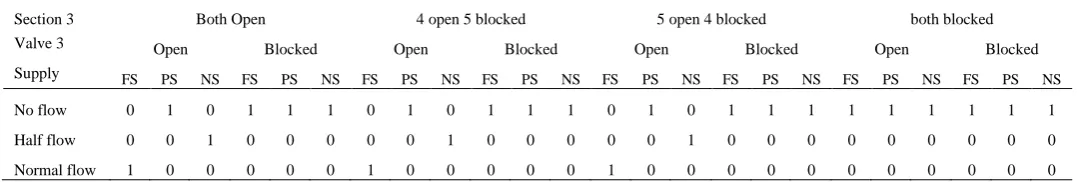
Finally, the intermediate nodes, and where re-quired, the component nodes, are connected to sensor nodes. Including the intermediate nodes reduced the size of the CPTs for the sensor nodes, in comparison to the CPTs without the intermediate nodes included in the BBN. For example, for sensors S5 – S11, the only information about the fuel supply required is the quantity supplied, but not which pump is supplying the fuel. Therefore, the CPTs for each of these sen-sors can be reduced to ¾ of the size by the introduc-tion of an intermediate node. The example CPT for sensor S11 is given in Table 3. In this table, FS stands for full supply (supply from both pumps), PS stands for partial supply (supply from one pump) and NS stands for no supply. This table demonstrates the re-duction in size of the CPT. Figure 2 is the BBN for the example system.
5.2.2 Discussion
The BBNs sensor nodes represent the sensors in the system. They produce sensor readings that corre-spond to the sensor readings that would be produced in a real system, assigning a state for each possible sensor reading. If there are too many different sensor readings that can be produced by each sensor, sensor readings may have to be grouped together into de-fined ranges. However, this would reduce the accu-racy of the modelling.
Including intermediate nodes reduced the overall size of the network as expected. However, it high-lighted the fact that even for a simple system, the size of the network was relatively large.
The BBN is used to aid in the diagnosis of failures in the system, as shown in the following section. 5.3 Fault diagnostics
Example component failures are diagnosed using the BBN in this section. As previously stated, the sen-sor combination used for fault diagnosis is one of the
Section 3 Both Open 4 open 5 blocked 5 open 4 blocked both blocked Valve 3 Open Blocked Open Blocked Open Blocked Open Blocked Supply FS PS NS FS PS NS FS PS NS FS PS NS FS PS NS FS PS NS FS PS NS FS PS NS
[image:6.595.312.562.261.371.2]No flow 0 1 0 1 1 1 0 1 0 1 1 1 0 1 0 1 1 1 1 1 1 1 1 1 Half flow 0 0 1 0 0 0 0 0 1 0 0 0 0 0 1 0 0 0 0 0 0 0 0 0 Normal flow 1 0 0 0 0 0 1 0 0 0 0 0 1 0 0 0 0 0 0 0 0 0 0 0
Figure 2 BBN of example system
[image:6.595.31.572.714.805.2]combinations of three sensors with the highest perfor-mance metric, sensors S1, S3 and S7. All combina-tions of 1 and 2 component failures were considered and the failed components were attempted to be diag-nosed using the fault diagnostic process.
All the failures in the system can be diagnosed with relative ease. In some cases, they are not diag-nosed correctly on the first attempt but no more than 2 components have to be inspected when only one component has failed, and no more than 3 compo-nents have to be inspected when 2 compocompo-nents have failed for the correct combination of component fail-ures to be found. This demonstrates that the model can diagnose the failures and the selected sensors are suitable.
The first case when failures aren’t diagnosed cor-rectly on the first attempt is when two different com-ponent failures produce the same symptoms. For ex-ample, pump P1 failed (or valve V1 failed) produce the same combination of sensor readings. In this ex-ample system, each component is equally likely to have caused the sensor readings, as all of the compo-nents have the same reliability. Therefore, it is not possible to definitely diagnose the correct component failure (pump P1 or valve V1) on the first inspection, the probability of diagnosing correctly the first time is 50%. However, if it is not diagnosed correctly on the first attempt, it can be diagnosed correctly when the second component is inspected.
The next case to be investigated is when the same sensor reading is produced for a single component failure and a combination of component failures, in-cluding the same single component failure. An ex-ample of this is when the fault diagnostic process di-agnoses the failure to be valve V3 failed. However, there is also the possibility that one of valve V4 or valve V5 is also failed, in addition to valve V3. These cases are significantly less likely than just valve V3 failed, but valve V4 (or V5) would be diagnosed as failed when valve V3 is repaired/replaced.
A similar situation arises if pump P1 or valve V1, or pump P2 or valve V2 are failed, in addition to valve V3. When valve V3 is repaired/replaced, this would then result in the same situation as described in para-graph 3 of this sub-section of the paper.
The final example is when the component failure is predicted to be valve V3 failed. If valves V1 and V2 are both failed, it produces the same sensor read-ings as if valve V3 is failed. However, the probability of this event occurring is significantly less than the probability of valve V3 failing. Therefore, the model will not diagnose the component failure (valve V1 and valve V2) correctly initially, but when further ev-idence is applied, i.e. valve V3 not failed, the correct component failures will be diagnosed. The example cases discussed above results in the diagnostic term (DI{s}) being less than 1, (0.6818).
The cases that were not diagnosed correctly ini-tially are because these combinations of component failures produce the same symptoms as other single component failures that are more likely to occur.
In the next section, an analysis of the methodology is given, along with potential improvements.
6 ANALYSIS OF THE PROPOSED METHODOLOGY
The first step of the methodology is to calculate the performance metric of the sensors. It has been ob-served that the BBN model has the potential to be used as the framework for calculating sensor perfor-mance metric automatically.
When component state evidence is introduced to the network, the sensor readings and the probability of the event can be produced automatically. If this is completed for all considered component failure com-binations, the performance metric can be calculated automatically. This removes the need to manually calculate the performance metric.
6.1 Sensor selection
In section 4.1.4, it was suggested that Equation 4 should be used as a guide for the initial sensor selec-tion, and then the individual terms of the performance metric should be used for the final selection of the sensors. This enables the analyst to favour specific terms of the performance metric, if desired. Consid-ering the three terms individually also helps to pre-vent the accidental selection of a sensor combination with one term significantly lower than desirable. 6.2 Modelling the system
The BBN model is a good representation of the ex-ample system. The BBNs sensor nodes output the sensor readings that represent a real system. How-ever, the system modelled is simplified, such as not considering partial failures, not considering block-ages in the lines and not considering leaks in the sys-tem. If these assumptions were to be removed, then the system representation would be more accurate. However, including these additional features in the BBN model would increase the size of the network significantly. If a significantly larger system is to be modelled accurately, this would result in very large BBNs. This could result in the networks being too large and it suggests that BBNs may not be scalable. Alternative modelling techniques will need to be con-sidered.
6.3 Fault diagnostics
There were some cases that the component failures were not diagnosed correctly initially, but when fur-ther evidence was introduced, these component fail-ures were correctly diagnosed. Examples of these cases were given in section 5.3.
A particular benefit of the BBN methodology used is that the results are the probabilities of each compo-nent failure. Therefore, if two most likely failures have a similar probability, both failures can be inves-tigated, for example, maintenance team could be in-formed of the most likely failures. This would reduce the overall downtime of the system, as both failures can be investigated at the same time, and repaired/re-placed as necessary.
7 CONCLUSIONS AND FUTURE WORK
In summary, a methodology to select the best com-bination of sensors using a newly developed perfor-mance metric was presented. The sensors were se-lected based on their ability to detect faults and diagnose failures, also considering the criticality of the failures detected. It was suggested that the three terms should be considered individually for the final selection of sensors. This would enable the user to select the best sensors based on the three different cri-teria.
A BBN based methodology was introduced to model the system and then diagnose component fail-ures using the selected sensors. Evidence was intro-duced in the BBN and the component failures diag-nosed. The outputs of the BBN can be used to rank the causes of sensor readings, which represent the faults on the system. The ranks can be used in mainte-nance prioritisation or mission reconfiguration in flight.
A few future research avenues could be explored. Firstly, the methodology needs to be tested on larger systems to check its applicability and the model scala-bility. This will require the performance metric cal-culation and sensor selection process to be automated in order for it to be completed within a reasonable time frame. Also, multiple system operation phases could be considered, such as phased missions which are observed on aircraft systems. These missions can consist of a number of individual phases such as take-off, cruise, fuel transfer and landing. This also ena-bles more component failure modes to be considered.
8 ACKNOWLEDGMENTS
This project is supported by British Aerospace Engi-neering (BAE) and the EngiEngi-neering and Physical Sci-ences Research Council (EPSRC). The authors grate-fully acknowledge the support of these organisations.
9 REFERENCES
Bartlett, L.M., Hurdle, E.E. and Kelly, E.M., (2006). Com-parison of digraph and fault tree based approaches for sys-tem fault diagnostics. Proceedings of the European Safety and Reliability Conference (ESREL 2006), Vol. 1, pp. 191-198.
Cheok, M.C., Parry, G.W., and Sherry, R.R., (1998) Use of importance measures in risk-informed regulatory appli-cations. Reliability Engineering & System Safety, 60(3), pp. 213-226.
Hurdle, E.E., Bartlett, L.M. and Andrews, J.D., (2007) Fault tree based fault diagnostics methodology for an air-craft fuel system. Proceedings of the 32nd ESREDA Sem-inar: Maintenance Modelling and Applications.
Hurdle, E.E., Bartlett, L.M. and Andrews, J.D., (2008). System fault diagnostics using fault tree analysis. Proceed-ings of the Institution of Mechanical Engineers, Part O: Journal of Risk and Reliability, 221 (1), pp. 43-55.
Lambert, J. H., & Farrington, M. W. (2007). Cost–benefit functions for the allocation of security sensors for air con-taminants. Reliability Engineering & System Safety,
92(7), pp.930-946.
Lampis, M. and Andrews, J. (2009). Bayesian belief net-works for system fault diagnostics. Quality and Reliability Engineering International, 25(4), pp.409-426.
Lloyd, M. D., Andrews, J. D., Remenyte-Prescott, R., Pearson, J. T., & Hubbard, P. (2014). A Petri Net Ap-proach to Fault Verification in Phased Mission Systems using the Standard Deviation Technique. Quality and Re-liability Engineering International, 30(1), pp.83-95.
Maul, W., Kopasakis, G., Santi, L., Sowers, T. and Chi-catelli, A. (2008). Sensor Selection and Optimization for Health Assessment of Aerospace Systems. Journal of
Aer-ospace Computing, Information, and Communication,
5(1), pp.16-34.
Pourali, M. and Mosleh, A. (2013). A Bayesian approach to sensor placement optimization and system reliability monitoring. Proceedings of the Institution of Mechanical Engineers, Part O: Journal of Risk and Reliability, 227(3), pp.327-347.
Santi, L. M., Sowers, T. S., & Aguilar, R. B. (2005). Opti-mal sensor selection for health monitoring systems,
Na-tional Aeronautics and Space Administration, 19(1),
pp.39-52.
Spanache, S., Escobet, T. & Travé-Massuyes, L., (2004). Sensor placement optimization using genetic algorithms. In 15th international Workshop on Principles of Diagnosis