c
ANALYTICAL GUARANTEES FOR REDUCED PRECISION FIXED-POINT MARGIN HYPERPLANE CLASSIFIERS
BY
CHARBEL SAKR
THESIS
Submitted in partial fulfillment of the requirements
for the degree of Master of Science in Electrical and Computer Engineering in the Graduate College of the
University of Illinois at Urbana-Champaign, 2017
Urbana, Illinois Adviser:
ABSTRACT
Margin hyperplane classifiers such as support vector machines are strong predictive models having gained considerable success in various classification tasks. Their conceptual simplicity makes them suitable candidates for the design of embedded machine learning systems. Their accuracy and resource utilization can effectively be traded off each other through precision. We analytically capture this trade-off by means of bounds on the precision re-quirements of general margin hyperplane classifiers. In addition, we propose a principled precision reduction scheme based on the trade-off between in-put and weight precisions. Our analysis is supported by simulation results illustrating the gains of our approach in terms of reducing resource utiliza-tion. For instance, we show that a linear margin classifier with precision assignment dictated by our approach and applied to the ‘two vs. four’ task of the MNIST dataset is ∼ 2× more accurate than a standard 8 bit low-precision implementation in spite of using ∼ 2×10⁴ fewer 1 bit full adders and ∼2×10³ fewer bits for data and weight representation.
ACKNOWLEDGMENTS
First and foremost, I would like to express my most sincere gratitude to my advisor, Professor Naresh Shanbhag. This work would have not been possible without his great guidance and the useful discussions we have had since I arrived at UIUC. Most importantly, I am very grateful to Prof. Shanbhag for encouraging me to explore the new and exciting area of machine learning in silicon.
I feel very lucky to have been mentored in my first year of graduate school by my friend Dr. Sai Zhang, from whom I have learned a lot. I am also very thankful to my friend Dr. Peter Kairouz, who helped me adapt to life at UIUC when I first joined.
None of the presented work would have been possible if it was not for the discussions and collaborations with my lab mates in the Shanbhag research group: Sujan Gonugondla, Ameya Patil, Dr. Yingyan Lin, Dr. Mingu Kang, Sungmin Lim, and Dr. Yongjune Kim.
Finally, I would like to express my deepest gratitude to my parents, Toufic and L´ena. I would never have achieved anything if it was not for all the sacrifices they have made for me. This thesis is dedicated to them.
TABLE OF CONTENTS
LIST OF TABLES . . . vi
LIST OF FIGURES . . . vii
LIST OF ABBREVIATIONS . . . viii
CHAPTER 1 INTRODUCTION . . . 1
1.1 Motivation . . . 1
1.2 Background . . . 2
1.3 Reduced Precision Machine Learning . . . 5
1.4 Contributions . . . 7
CHAPTER 2 PRECISION ANALYSIS OF FIXED-POINT HY-PERPLANE CLASSIFIERS . . . 9
2.1 Classifier Precision . . . 9
2.2 Precision in Training . . . 16
2.3 Addendum: Proofs and Boundary Cases . . . 18
2.4 Summary . . . 22
CHAPTER 3 SIMULATION RESULTS . . . 23
3.1 Complexity in Fixed-Point . . . 23
3.2 Validation of Bounds . . . 24
3.3 Complexity vs. Accuracy Trade-offs . . . 27
3.4 Training Behavior . . . 30
3.5 Summary . . . 33
CHAPTER 4 CONCLUSION . . . 34
LIST OF TABLES
2.1 Table of GLBs for linear, NLIM, NLOM, and quadratic
form classifiers. . . 12 2.2 List of E1 andE2 appearing in the PUB for linear, NLIM,
NLOM, and quadratic form classifiers. . . 14 2.3 Output quantization noise and its upper bounded needed
to prove the GLB for each classifier type. . . 18 2.4 Input and weight quantization noise variances referred to
output and classifier floating-point output. . . 20 3.1 Summary of Fig. 3.1 illustrating minimum precision
re-quirements for hyperplane classifiers on the Breast Cancer
Dataset. . . 26 3.2 Results for the Breast Cancer Dataset. Comparison of
computational cost, representational cost, and test error
for all classifier types. . . 29 3.3 Results for linear classification on the ‘two vs. four’ task for
the MNIST Dataset. Comparison of computational cost,
LIST OF FIGURES
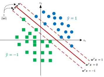
1.1 Illustration of the geometry of a margin hyperplane classifier. . 2
1.2 Architectures of various margin hyperplane classifiers. . . 6
2.1 Illustration of the GLB for a linear classifier. . . 11
2.2 Comparison of the GLB across classifier types. . . 13
3.1 Results for classification on the Breast Cancer Dataset. . . 25
3.2 Results for linear classification on the ‘two vs. four’ task for the MNIST Dataset. . . 27
3.3 Results for linear classifier training on the Breast Cancer Dataset. . . 31
3.4 Results for quadratic form classifier training on the Breast Cancer Dataset. . . 32
3.5 Results for linear classifier training on the ‘two vs. four’ task for the MNIST Dataset. . . 33
LIST OF ABBREVIATIONS
CPU Central Processing Unit
DP Dot Product
FA Full Adder
FL Sim Floating-point Simulation FX Sim Fixed-point Simulation GLB Geometric Lower Bound GPU Graphics Processing Unit LMS Least Mean Square MAC Multiply and Accumulate
MNIST Modified National Institute of Standards and Technology Database MVM Matrix Vector Multiplication
NLIM Non-Linear Input Mapping NLOM Non-Linear Output Mapping PUB Probabilistic Upper Bound RBF Radial Basis Function SGD Stochastic Gradient Descent
SQNR Signal-to-Quantization Noise Ratio SVM Support Vector Machine
TP Tensor Product
CHAPTER 1
INTRODUCTION
1.1
Motivation
Because of their high computational and storage complexity, today, machine learning systems are deployed in the cloud and on large-scale general-purpose computing platforms such as CPU and GPU-based clusters [1]. A key chal-lenge today is to incorporate inference capabilities into untethered (embed-ded) platforms such as cell phones, autonomous unmanned vehicles, and wearables. Such platforms, however, have stringent limits on available en-ergy, computation, and storage resources. Enabling such on-device intelli-gence necessitates a fresh look at the design of resource-constrained learning algorithms and architectures.
Precision of data, weight vector, and internal signal representations in a machine learning implementation have a profound impact on its overall com-plexity. Not surprisingly, recent works have empirically studied the effect of moderate [2] and heavy [3–6] quantization on the performance of learning systems. Signal-to-quantization noise ratio (SQNR) has also been used as a metric to understand precision-accuracy trade-offs for the forward path [7] and training [8] of deep neural networks. These works raise the following questions: Is there a systematic way of choosing the minimum precision of data, weights, and internal signal representations? Are these precisions inter-dependent? How should one choose the precision of the training algorithm? Our work addresses these questions for the general case of margin hyperplane classifiers.
In fact, the questions listed above have been answered for the popular least mean-squared (LMS) adaptive filter [9–15] in the context of digital signal processing and communications systems. It turns out that there is a trade-off between data and coefficient precision in order to achieve a desired
Figure 1.1: Illustration of the geometry of a margin hyperplane classifier.
SQNR at the output. Furthermore, the precision of the LMS weight update block needs to be greater than that of the coefficient in the filter to avoid a premature termination of the convergence process. This thesis leverages these insights in the design of fixed-point machine learning algorithms.
1.2
Background
1.2.1
The Classification Problem
Given a feature vector x of dimension D, with a corresponding unknown true labely ∈ {±1}, it is desired to predict the class it belongs to. There are several approaches to solving the problem, amongst which are hyperplane classifiers. These separate the feature space by means of a hyperplane and assign a predicted label ˆy based on the relative position of the feature vector with respect to the hyperplane. For generalizability, it is often desired to determine a maximum margin separating hyperplane in the feature space (see Fig. 1.1) as is the case for SVMs [16]. The classifier is said to have a soft margin when some of the feature vectors are allowed to lie within the margin and hence may be misclassified.
the label as follows: wTx+b ˆ y=1 R ˆ y=−1 0 (1.1)
where w is the weight vector and b is the bias term. For notational conve-nience, we reformulate (1.1) into an equivalent affine form:
wTx ˆ y=1 R ˆ y=−1 0 (1.2)
by absorbing the bias termbinto the weight vector and extending the feature space by one: w←hb wTiT andx←h1 xTiT. Often, data statistics make the classification problem linearly non-separable in the input feature space. To circumvent this issue, one method is to map the input feature space to a higher dimension, i.e., x → φ(x) such that it becomes linearly separable, i.e.: wTφ(x) ˆ y=1 R ˆ y=−1 0 (1.3)
We refer to this method as non-linear input mapping (NLIM). The non-linear map φ(x) typically lifts the data to a much higher dimension. Consequently, the dimension of the weight vector w in (1.3) is greater than that in (1.2).
Sometimes, it is impractical to map the input into a space where the data is linearly separable. The reason is that the corresponding dimension may be too large or even infinite. A remedy to this problem is the popular kernel trick which we refer to as non-linear output mapping (NLOM). The idea is to perform the similarity operation (projection, distance, etc.) in the original (lower dimensional) feature space and then apply a kernel to the result, as shown below: Ns X i=1 αiK(si,x) +b ˆ y=1 R ˆ y=−1 0 (1.4)
where K(·,·) is the kernel, b is a bias term, si’s are called support vectors, and αi’s are the Ns constants associated with the Ns support vectors. The support vectors found during training characterize the margin of the sepa-rating region. Their number depends on the size of the training set and the dimensionality of the input and output spaces. Note that since the support vectors are obtained through training, it is not possible to absorb the bias term into the kernel in a similar fashion as in (1.2).
For the dot product kernel K(si,x) = sTi x, it can be seen that (1.2) and (1.4) are identical by letting w = PNs
i=1αisi and extending the feature
space by one. A slightly more sophisticated kernel is the polynomial kernel:
K(si,x) = (sTix)d where d is the order of the polynomial. Another popular kernel is the radial basis function (RBF):K(si,x) = exp(−12ksi−xk
2
). This kernel maps the data into an infinite-dimensional space.
In [17], a reformulation for the second order polynomial kernel SVM was proposed. Essentially, using the fact that (siTx)2 = xT(sisTi )x, one can reformulate (1.4) as: xTKx ˆ y=1 R ˆ y=−1 0 (1.5) where K = PNs i=1αisis T
i . Note that extending the feature space by one allowed us to absorb the bias term into the matrix K. This reformulation is attractive for of two reasons: (1) the computational cost reduces from Ns inner products in RD to D+ 1 inner products in RD (typically N
s D); (2) there is no need to store any support vectors.
1.2.2
Learning Classifier Parameters
It is possible to train hyperplane margin classifiers on the fly using the stochastic gradient descent (SGD) algorithm. For a linear classifier, the in-stantaneous loss function is:
Q(yn,xn,w) = λkwk2+ max{0,1−ynwTxn} (1.6) whereynis the true label corresponding to thenthsamplexn. The hinge loss term in (1.6) contributes to the margin and λ is a regularizer. The optimum weight vector w that minimizes this loss function can be determined using SGD via the following updates [18]:
wn+1 = (1−γ λ)wn+ 0 if ynwTnxn>1, γ yn xn otherwise (1.7)
For NLIM classifiers, the weights can be trained in a similar manner as follows: wn+1 = (1−γ λ)wn+ 0 if ynwTnφ(xn)>1, γ yn φ(xn) otherwise (1.8)
For NLOM classifiers, we will consider only the decision directed mode. This is because NLOM requires knowledge of the support vectors that arise during training, and hence obtaining an SGD procedure to train such a system is difficult.
Finally, the quadratic form of (1.5) suggests a straightforward SGD train-ing method. Indeed, as the gradient∇K xTKx
=xxT, the update equation is given by: Kn+1 = (1−γ λ)Kn+ 0 if ynxTnKxn >1, γ yn xnxTn otherwise (1.9)
where L2 regularization is applied to K.
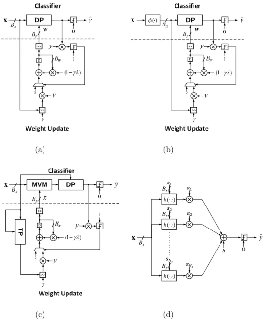
Figure 1.2 depicts the architectures of the various classifiers considered with online training weight update blocks shown for linear, NLIM, and quadratic form classifiers. The multiplications and additions are element-wise. The precision assignment per dimension for each signal considered in the upcoming analysis is highlighted. These are input precision BX, weight precision BF, and weight update precision BW. In this thesis, we obtain bounds on these precisions in order to achieve a desired level of accuracy.
1.3
Reduced Precision Machine Learning
Traditional high-precision computations implemented in modern CPUs em-ploy 64 bit floating-point representations and arithmetic. In the past decade, GPUs have gained increased popularity as machine learning accelerators thanks to their parallelization capabilities. Most GPUs employ 32 bit floating-point representations and arithmetic. Such high precision severely impacts the costs of computation, storage, and communications associated with the implementations of machine learning algorithms. Understandably, there has been a wave of research in the recent past that considers other models of
DP >> >> D (a) DP >> >> D (b) MVM >> >> DP TP D (c) X B x 0 ˆ y F B F B F B (d)
Figure 1.2: Architectures of various margin hyperplane classifiers showing the precision assignments per dimension, and the classifier and weight update blocks for: (a) linear, (b) NLIM, (c) quadratic form, and (d) the NLOM classifier. DP denotes a dot product block, MVM denotes a matrix vector multiplier, and TP denotes a tensor product block.
computations and representations at much lower precisions.
A common approach to representing and computing in reduced precision is to employ fixed-point quantization [19]. This approach was used in some popular machine learning accelerators such as Eyeriss [20], the Diannao fam-ily [21], and Google’s tensor processing unit (TPU) [22]. In fixed-point,
quantization levels are scattered uniformly across the quantization domain. Fixed-point implementations are attractive because they are efficient. Fur-thermore, one advantage of fixed-point quantization is the extensive work on quantization noise analysis [9, 10, 23] generally allowing for an intuitive un-derstanding of the precision requirements of machine learning algorithms [19] as will be shown in the remainder of this thesis.
One possibility is to consider reduced precision floating-point representa-tions. While it has not been thoroughly investigated as of today, floating-point quantization seems promising due to its better dynamic range, making it more robust at the algorithm level. The main difficulty remains in the multiplicative noise model traditionally considered [23, 24]. Such a model is both pessimistic and mathematically less tractable than that of fixed-point quantization noise. Furthermore, the costs of implementing reduced preci-sion floating-point algorithms are comparable to fixed-point implementations, giving the former no clear advantage.
Recently, some empirical works have demonstrated the possibility of using extreme measures in reduced precision. Those include log quantization or power of 2 quantization [25], binarization [5], and ternarization [26]. Such approaches seem to reduce the costs of implementation by a great deal; nev-ertheless, it is observed that the deployment of such quantization schemes is only made possible through algorithmic extensions rendering the overall complexity worse than a fixed-point counterpart [27]. In addition, the effects of those quantization methodologies are still not well understood analytically. Hence, in the remainder of this thesis we shall focus on reduced fixed-point precision in the context of the design and implementation of hyperplane clas-sifiers.
1.4
Contributions
In this thesis, we propose an analytical framework to predict precision vs. accuracy trade-offs in the design of fixed-point learning algorithms thereby eliminating the need for trial-and-error. A simplified version of this work, addressing the issue of fixed-point linear support vector machines (SVM), can be found in [19]. Those results are extended in this thesis to obtain a complete and rigorous set of bounds for general margin hyperplane classifiers.
Specifically, we consider classifiers using non-linear input mapping (NLIM), non-linear output mapping (NLOM), also known as kernels, and quadratic forms. We analyze the trade-off between data and weight precisions. In addition, we propose a principled approach to reduce the precision of various algorithmic parameters while maintaining fidelity to the ideal (floating-point) accuracy. We quantify the benefits of this precision reduction in terms of computational (# of 1 b full adders) and representational (# of bits) costs. We test and validate all our results through simulations on the Breast Cancer Dataset from the UCI Machine Learning Repository [28] and the MNIST Dataset for handwritten character recognition [29].
CHAPTER 2
PRECISION ANALYSIS OF FIXED-POINT
HYPERPLANE CLASSIFIERS
2.1
Classifier Precision
In this section, we assume that the classifier has been pretrained in floating-point and we analytically study how much can it be quantized and how its accuracy varies with its precision. In our analysis, we assume without loss of generality that all quantities of interest lie between ±1. This can be achieved for data via scaling and for the weights by forcing saturation upon each iteration. Finally, unless otherwise stated, we allow the precision of internal signals to grow arbitrarily. That is, we do not incorporate inter-mediate round-offs in our analysis. The bit growth phenomenon only adds a logarithmic term to the computational complexity. The upcoming analy-sis can be extended by considering round-off noise terms but would become much less tractable. Figure 1.1 shows the geometric configuration of a mar-gin hyperplane classifier. This illustration reveals interesting insights upon which we build our analysis.
2.1.1
Geometric Lower Bounds
The first result exploits the geometry of the classifier to provide a lower bound on the precision which guarantees that the quantized feature vec-tors lying outside the margin are classified correctly. The geometric lower bounds (GLB) are conservative in the sense that they are sufficient conditions for fixed-point classifiers to have an average accuracy close to their trained floating-point counterparts.
Finite precision computation modifies (1.2) to: (w+qw)T(x+qx) ˆ y=1 R ˆ y=−1 0 (2.1)
where qx ∈ RD and qw ∈ RD are the quantization noise terms in x and w respectively. Each element of qx, except the first one, is a random variable uniformly distributed with support [−∆X
2 , ∆X
2 ], where ∆X = 2
−(BX−1) is the
input quantization step. The first term inqx is zero. Similarly, each element of qw is a random variable uniformly distributed with support [−∆2F,∆2F], where ∆F = 2−(BF−1) is the coefficient quantization step. This uniform as-sumption is standard [10], has been found to be accurate in signal processing and communications systems, and is validated by the experimental results in our thesis. Note that quantization perturbs both the feature vector xand the separating hyperplane defined by w.
In what follows, for a feature vector x, let us denote by ˆyf l(x) the label predicted by the floating-point classifier and by ˆyf x(x) the one predicted by the corresponding fixed-point classifier. The notation a denotes a vector a
without the first element. We start with the linear classifier and consider the GLB on BX.
Theorem 1 (Geometric Lower Bound onBX for a Linear Classifier). Given BF, and w, ∀x∈ RD such that |wTx|>1, yˆf x(x) = ˆyf l(x) if
BX >log2 || w||√D−1 1−2−BF||x|| √ D (2.2) where BF >log2 ||x||√D.
Proof. See this chapter’s addendum (Section 2.3.1).
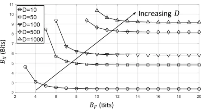
The GLB for a linear classifier reveals the following insights: (1) larger margin (i.e., smaller ||w|| in Fig. 1.1) allows a greater reduction of BX, (2) there is a trade-off betweenBX andBF, and (3) input precisionBX increases with dimensionD and||x||. Figure 2.1 shows the trade-off betweenBX and
BF for several values of the dimensionD. In each case, the starting value of
BF corresponds to the condition of Theorem 1.
Note that Theorem 1 is specific to a single feature vector x and can be extended to a dataset.
(Bi
ts
)
(Bits)
Increasing
Figure 2.1: Illustration of the GLB for a linear classifier showing trade-off between input (BX) and weight (BF) precisions, and dependence on the dimension (D). In this example, the values of||w|| and||x||are taken to be the mean norm of the corresponding vectors assuming each entry is random and uniformly distributed between -1 and 1.
Corollary 1.1 (Geometric Lower Bound onBX for a Linear Classifier on a Dataset).
Given BF, and w, ∀x∈ RD such that |wTx|>1, yˆf x(x) = ˆyf l(x) if
BX >log2 ||w||√D−1 1−2−BFmax x∈X ||x|| √ D (2.3) where BF >log2 max x∈X ||x|| √ D .
In Table 2.1, we list the GLB for the different classifiers. These lower bounds on precision guarantee that any feature vector lying outside the mar-gin of a floating-point classifier is identically classified by the fixed-point counterpart. The GLB is a guideline on the safe exploitation of the margin. Note that we may derive a GLB on BX given BF or onBF given BX. Each of these GLBs can be extended for a classifier operating on a dataset as in Corollary 1.1. Please refer to this chapter’s addendum (Section 2.3.1) for the proofs.
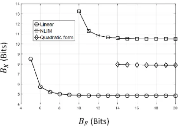
Figure 2.2 shows a comparison across linear, NLIM, and quadratic form classifiers. It appears that the NLIM classifier has the highest input precision requirement, followed by the quadratic form and linear classifiers, in that or-der. The quadratic form classifier seems to have the highest weight precision requirement.
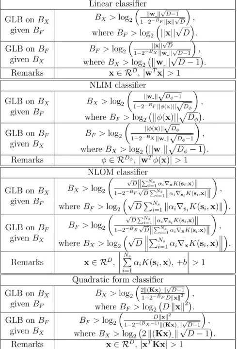
Table 2.1: Table of GLBs for linear, NLIM, NLOM, and quadratic form clas-sifiers. The classifier parameters, for each case, are as defined in Section 1.2. The precision assignments are as shown in Fig. 1.2. Under these conditions we have ˆyf x(x) = ˆyf l(x). The first row identical to Theorem 1. The proofs of these bounds can be found in this chapter’s addendum (Section 2.3.1).
Linear classifier GLB on BX given BF BX >log2 || w||√D−1 1−2−BF||x||√D , where BF >log2 ||x||√D . GLB onBF given BX BF >log2 || x||√D 1−2−BX||w||√D−1 , where BX >log2 ||w|| √ D−1. Remarks x∈ RD, |wTx|>1 NLIM classifier GLB on BX given BF BX >log2 ||w||√Dφ−1 1−2−BF||φ(x)||√Dφ , where BF >log2 ||φ(x)|| p Dφ . GLB onBF given BX BF >log2 ||φ(x)||√Dφ 1−2−BX||w||√Dφ−1 , where BX >log2 ||w|| p Dφ−1 . Remarks φ∈ RDφ, |wTφ(x)|>1 NLOM classifier GLB on BX given BF BX >log2 √ DkPNs i=1αi∇xK(si,x)k 1−2−BF√DPNs i=1kαi∇siK(si,x)k , where BF >log2 √ DPNs i=1kαi∇siK(si,x)k . GLB onBF given BX BF >log2 √ DPNs i=1kαi∇siK(si,x)k 1−2−BX√DkPNs i=1αi∇xK(si,x)k , where BX >log2 √ D PNs i=1αi∇xK(si,x) . Remarks x∈ RD, Ns P i=1 αiK(si,x), +b >1 Quadratic form classifier
GLB on BX given BF BX >log2 2k(Kx)k√D−1 1−2−BFDkxk2 , where BF >log2 Dkxk 2 . GLB onBF given BX BF >log2 Dkxk2 1−2−(BX−1)k(Kx)k√D−1 , whereBX >log2 2k(Kx)k √ D−1. Remarks x∈ RD,|xTKx|>1
Figure 2.2: Comparison of the GLB across classifier types. The input di-mension is arbitrarily chosen to be D = 50. For the NLIM classifier, the map considered is the second order polynomial one (Dφ = D2). For each case, inputs and weights are random, uniformly distributed between -1 and 1, per dimension. To obtain average bounds, 1000 datasets are generated. The GLBs plotted are the mean bounds in each case.
2.1.2
Probabilistic Upper Bounds
The GLB provides a lower bound on the precision requirements to ensure that fixed-point decisions are identical to floating-point for feature vectors lying outside the margin of the classifier. However, it does not provide quantitative guarantees on the fixed-point accuracy. Probabilistic upper bounds (PUBs), introduced next, upper bound the worst-case fixed-point accuracy for a given precision.
In what follows, we employ capital letters for random variables. We define probability of mismatchpm between the decisions made by the floating-point and fixed-point algorithms aspm = Pr{Yˆf x 6= ˆYf l}, where ˆYf xis the output of the fixed-point classifier and ˆYf l is the output of the floating-point classifier. A small mismatch probability indicates that the classification accuracy of the fixed-point algorithm is very close to that of the floating-point algorithm. Indeed, if we know the accuracy of the floating-point system quantified by its probability of error pe,f l = Pr{Yˆf l 6=Y} (Y is the true output), then we can obtain an upper bound on the fixed-point probability of error pe,f x = Pr{Yˆf x 6=Y}:
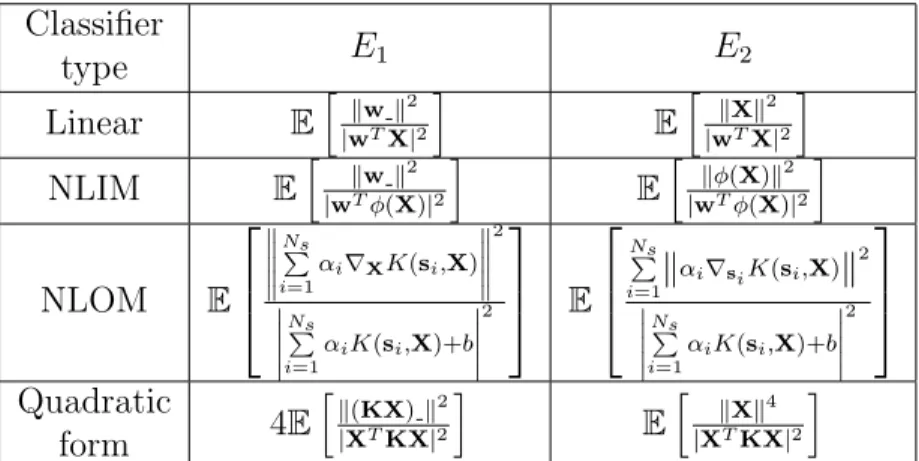
Table 2.2: List of E1 and E2 appearing in the PUB (Theorem 2) for linear,
NLIM, NLOM, and quadratic form classifiers. For each case, the classifier parameters, as defined in Section 1.2, are pre-trained in floating-point. The expectations are taken over random inputs. The precision assignments are as shown in Figure 1.2. Classifier type E1 E2 Linear Eh|wkwTXk2|2 i E h k Xk2 |wTX|2 i NLIM Eh|wkTwφ(kX2)|2 i E h kφ(X)k2 |wTφ(X)|2 i NLOM E Ns P i=1 αi∇XK(si,X) 2 Ns P i=1 αiK(si,X)+b 2 E Ns P i=1k αi∇siK(si,X)k 2 Ns P i=1 αiK(si,X)+b 2 Quadratic form 4E hk (KX)k2 |XTKX|2 i E h k Xk4 |XTKX|2 i
Proposition 1. The fixed-point probability of error is upper bounded as fol-lows:
pe,f x ≤pe,f l+pm (2.4)
The right-hand side represents the union bound of two events: (1) misclas-sification, and (2) incorrect classification due to quantization.
Note that pe,f x is the quantity of interest as it characterizes the accuracy of the fixed-point system. While pe,f l is a metric of the algorithm itself and does not depend on quantization, pm is the term that captures the impact of quantization on accuracy and we hence use it as a proxy for pe,f x in order to evaluate the accuracy of a fixed-point system. In what follows, we obtain analytical upper bounds onpmas a function of the precision of the fixed-point system.
It turns out that, for all the classifiers considered in Fig. 1.2, the mismatch probability pm is upper bounded as follows:
Theorem 2 (Probabilistic Upper Bound on pm). Given BX and BF, the upper bound on the mismatch probability of a hyperplane classifier is given by: pm ≤ 1 24 ∆ 2 XE1+ ∆2FE2 (2.5) where, for each case, the values of E1 and E2 are listed in Table 2.2.
In practice, the statistics (i.e., the expected valuesE1 and E2 in (2.5)) are
calculated empirically. Note that the mismatch probability bound is increas-ing in ∆X and ∆F, which is expected as higher quantization noise variance leads to increased mismatch between fixed and floating-point algorithms.
Equation (2.5) reveals an interesting trade-off between input precisionBX and weight precision BF. Indeed, in (2.5), the first term, ∆2XE1, is the
input quantization noise power gain while the second, ∆2FE2, is the weight
quantization noise power gain. Depending on the values taken by E1 and E2, it might be that one of the two terms dominates the sum. If so, then it would imply that BF orBX is unnecessarily large and hence can be reduced without increasingpm. An intuitive first step to obtain a tighter upper bound is to make the two terms of comparable order, i.e., set ∆2
XE1 = ∆2FE2 by
constraining BX and BF as follows:
BX −BF =round log2 r E1 E2 ! (2.6) where round() denotes the rounding operation. This is an effective way to handle one of the two degrees of freedom introduced by (2.5).
One way to employ (2.6) is to consider minimizing the upper bound in (2.5) subject to the constraint BX +BF =c for some constant c. Indeed, it can be shown that (2.6) would be a necessary condition of the corresponding solution.
From the expressions ofE1 andE2 in Table 2.2 we note two points. First,
for each classifier, the denominator within the expectation operator repre-sents the confidence in classification. This means that, the better the clas-sifier separates the data, the smaller E1 and E2 are expected to be. Hence,
better data separability implies better tolerance to quantization, which is to be expected. Second, the numerators represent functions of the magnitudes of weight and input vectors in the decision space. Such magnitudes are di-rect functions of dimensionality and margin. Consequently, we may infer that higher dimensionality, or smaller margin, increases the values of E1 and E2,
and hence leads to an increase in the precision requirements of the classifier. This correlates well with our observations in the case of the GLB.
The results presented in this section provide useful insights to determine suitable precision allocations for inputs and weights. First, the GLBs offer
a condition under which the behavior of a fixed-point system is expected to be similar to that of the corresponding floating-point one. However, they do not provide analytical guarantees on the resulting accuracy. The PUBs do, and (2.6) captures an interesting trade-off between both precisions. In practice, it is possible to use both sets of bounds to efficiently determine minimal precisions for a fixed-point implementation. For example, (2.6) can first be used to determine the optimal difference between BX and BF, then the GLB can be used to find a suitable pair of (BX, BF). Finally, the PUB can be used to estimate the expected accuracy loss. We shall demonstrate this approach in Chapter 3.
2.2
Precision in Training
In the preceding discussion, all learning parameters were assumed to have been obtained after full-precision training. In practice, it is standard to first implement a floating-point algorithm with desirable convergence properties and then quantize so as to preserve the convergence behavior unaltered. In this section, we consider the problem of finding precision requirements on
BW in the updates when training is done in fixed-point with feedforward precisions set to BX and BF.
Consider a linear classifier. Note that the right-hand side of (1.7) includes an attenuation term (1−γ λ)wnand an update term equal to 0 orγ ynxn= ±γxn where xi ∈ [−1,1] for i = 1. . . D. Without loss of generality, we assume that floating point convergence is achieved for λ= 1 and some small value of γ. Therefore, the attenuation factor (1−γ λ) is less than or close to unity independent of BW.
Our next result ensures that the non-zero update term in (1.7) is non-zero during training in spite of weight update quantization.
Theorem 3 (Weight Update Requirements for a Linear Classifier).
The following lower bound on weight update precision BW is a sufficient condition to ensure full convergence:
BW ≥BX −log2(γ) (2.7)
Proof. Each step in (1.7) has magnitude |γx| wherexis a scalar value taken by the different components of x. For any zero update to remain non-zero after quantization, we need |γx| > 12bmin where bmin = 2−(BW−1) is the value of the least significant bit (LSB) in the weight update block. So we require |γ||x|> 122−(BW−1) = 2−BW. This has to be satisfied for any non-zero
value of x, but the minimum non-zero value taken by |x| is 2−(BX−1). So we
get |γ| ·2−(BX−1) >2−BW, which can be written as:
BW > BX −1−log2(γ)⇔BW ≥BX −log2(γ)
Theorem 3 provides a sufficient condition for convergence. As the SGD approximates the true gradient at every step, fewer bits than specified in (2.7) may work occasionally. We refer to these as boundary cases and present a detailed analysis of the corresponding learning behavior in this chapter’s addendum (Section 2.3.3).
For a NLIM classifier, the exact same discussion applies. This is because (1.7) and (1.8) are structurally equivalent. For a quadratic form classifier the results change a little bit. Indeed, every entry (i, j) in the matrix K has an update term equal to |γxixj| in absolute value. The product of two scalars increases the precision by a factor of 2. Following the same argument as in Theorem 3, we have the following result:
Corollary 3.1 (Weight Update Requirements for a Quadratic Form Classi-fier).
The following lower bound on weight update precisionBW is a sufficient con-dition to ensure full convergence:
BW ≥2BX −log2(γ) (2.8)
when BX and BF are the input and coefficient precisions, respectively.
While the required precision for full convergence has been slightly modified in this case, the discussion of the learning behavior for lower precisions is exactly the same as that following Theorem 3. This is because that discussion observes the inputs starting from the most significant bit (MSB) and towards the LSB. The set [−1,1] being closed under multiplication, the update terms
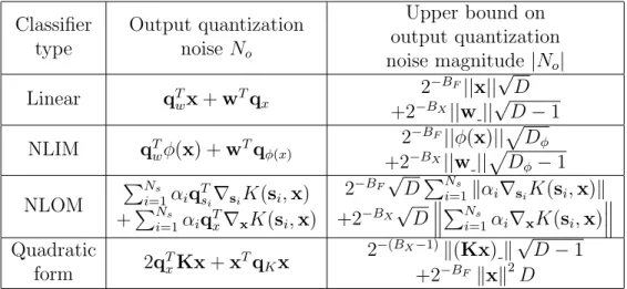
Table 2.3: Output quantization noise No and corresponding upper bounds on its magnitude needed to prove the GLB for each classifier type. Note that
qx,qw, qφ(x),qsi,qK are the quantization noise terms of x, w,φ(x),si, and
K, respectively. Classifier type Output quantization noise No Upper bound on output quantization noise magnitude |No| Linear qTwx+wTqx 2−BF||x|| √ D +2−BX||w||√D−1 NLIM qT wφ(x) +wTqφ(x) 2−BF||φ(x)||pD φ +2−BX||w||pD φ−1 NLOM PNs i=1αiq T si∇siK(si,x) +PNs i=1αiq T x∇xK(si,x) 2−BF√DPNs i=1kαi∇siK(si,x)k +2−BX √ D PNs i=1αi∇xK(si,x) Quadratic form 2q T xKx+xTqKx 2−(BX−1)k(Kx)k√D−1 +2−BFkxk2D
are just as significant as those in the case of a linear classifier when looking at the MSB and onwards.
2.3
Addendum: Proofs and Boundary Cases
2.3.1
Proofs of Geometric Lower Bounds
The proof of the GLB is done in three steps:
• Step 1: Determine the output quantization noise No at the output of the classifier. In this step, we neglect cross products of quantization noise terms as their contribution is very small. For the NLOM classifier, this is equivalent to a first order Taylor expansion on the kernel. For the linear classifier we have:
No =qTwx+w T
qx
• Step 2: Upper bound the magnitude of No using the triangle and Cauchy-Schwarz inequalities. Input quantization noise terms are upper bounded by 2−BX and weight quantization noise terms by 2−BF. For
the linear classifier we have: |No| ≤ |qTwx|+|w T qx| ≤ kqwk kxk+kwk kqxk ≤2−BF||x|| √ D+ 2−BX||w||√D−1.
• Step 3: Set the upper bound on |No| to be less than the functional margin of the classifier which is equal to 1 (see Fig. 1.1).
Step 3, up to a rearrangement of terms, is equivalent to the GLB as de-scribed in Section 2.1. In Table 2.3, we list the output quantization noise and corresponding upper bound for each classifier type.
2.3.2
Proofs of Probabilistic Upper Bounds
The PUB is proved in 4 steps:
• Step 1: For a single input, obtain the total output quantization noise
No. This is identical to the Step 1 in the proof of the GLB above. This output quantization noise is a sum of independent input and weight quantization noise terms.
• Step 2: Compute the variance (σ2
No) of this output quantization noise.
Because of independence, it is the sum of the input (σ2
qx→o) and weight
(σq2w→o) quantization noise variances referred to the output. For the linear classifier we have:
σ2No = ∆ 2 X 12 ||w|| 2 +∆ 2 F 12||x|| 2
• Step 3: Use this computed variance and Chebyshev’s inequality to de-termine the probability of the quantization noise being larger in mag-nitude than the floating-point soft output zo of the classifier. Because the quantization noise has a symmetric distribution, this probability needs to be divided by 2 (the mismatch is only caused when quantiza-tion noise and output have opposing signs). The upper bound is hence
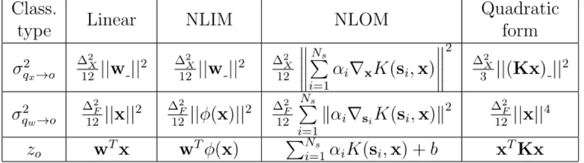
Table 2.4: Input (σq2x→o) and weight (σ2qw→o) quantization noise variances referred to output and classifier floating-point output (zo).
Class.
type Linear NLIM NLOM
Quadratic form σ2 qx→o ∆2 X 12||w|| 2 ∆2X 12 ||w|| 2 ∆2X 12 Ns P i=1 αi∇xK(si,x) 2 ∆2 X 3 ||(Kx)|| 2 σ2 qw→o ∆2F 12||x|| 2 ∆2F 12||φ(x)|| 2 ∆2F 12 Ns P i=1 kαi∇siK(si,x)k 2 ∆2F 12||x|| 4 zo wTx wTφ(x) PNs i=1αiK(si,x) +b xTKx derived as follows: pm = 1 2P(|No|>|zo|)≤ σN2o 2|zo|2 = σ 2 qx→o+σ 2 qw→o 2|zo|2
• Step 4: Use the law of total probability over the data to obtain the averaged upper bound on pm. For the linear classifier we obtain:
pm ≤ ∆2 X 24E " kwk2 |wTX|2 # +∆ 2 F 24E " kXk2 |wTX|2 #
For each classifier type, we list the values of σ2
qx→o, σ 2
qw→o, and zo in Table
2.4. The values of E1 and E2 in Table 2.2 are equal to ∆122
XE hσ2 qx→o |Zo|2 i and 12 ∆2 FE hσ2 qw→o |Zo|2 i
for each classifier type, respectively.
For the quadratic form case, we used the fact that, for a datapoint x,
V ar(xTqKx) =
∆2
F 12 kxk
4
. This result is proved as follows:
V ar(xTqKx) =E (xTqKx)2 =xTEqKxxTqTK x =xTE qTK,1x .. . qT K,Dx h qT K,1x . . . qTK,Dx i x =xT∆ 2 F 12 kxk 2 ID×Dx= ∆2 F 12 kxk 4 where qT
K,i for i= 1. . . D are the row vectors ofqK and ID×D is the identity matrix of size D×D. The fourth equality holds because the quantization terms are independent of each other making the off-diagonal elements of the matrix in the third equation a product of two zero-mean independent terms.
2.3.3
Precision of Training for Boundary Cases
We analyze the learning behavior when the precision is less than the one predicted by Theorem 3.
As 1−γλ ≈1, we assume (1−γλ)wi,n≈wi,nfori= 1. . . D. LetK =BW and M = BX. Let ˜xi,n = ynxn be the update term per dimension. The following cases describe the corresponding two’s complement arithmetic:
Case 1:BW = 1−log2(γ)⇔γ = 2−(BW−1) then:
γ = 0 .0 . . . 1 wi,n = bw0 .bw1 . . . bwK−1 γx˜i,n = bx0 .bx0 . . . bx0 bx1. . . bxM−1 where {bwi} K−1 i=0 and {bxi} M−1
i=0 are the binary expansions of wi,n and xi,n, respectively. Hence, if ˜xi,n ≥ 0→ wi,n+1 =wi,n, and if ˜xi,n <0 → wi,n+1 = wi,n−γ. We hence obtain a sign-SGD behavior only when ˜xi,n<0. Therefore, in case I, there is no way to guarantee convergence.
Case 2:BW = 2−log2(γ)⇔γ = 2−(BW−2) then:
γ = 0 .0 . . . 1 0
wi,n= bw0 .bw1 . . . bwK−2 bwK−1
γx˜i,n= bx0 .bx0 . . . bx0 bx1 bx2. . . bxM−1
Hence, ˜xi,n ≥ 0.5 → wi,n+1 = wi,n+ 0.5γ, 0 ≤ x˜i,n < 0.5 → wi,n+1 = wi,n, −0.5 ≤ x˜i,n < 0 → wi,n+1 = wi,n−0.5γ, and, −1 ≤ x˜i,n < 0.5 → wi,n+1 = wi,n−γ. We get a more precise but very noisy estimate of the gradient. We may observe inaccurate convergence.
Case 3:BW =−log2(γ)⇔γ = 2−BW then:
γ = 0 .0 . . . 0 1
wi,n = bw0 .bw1 . . . bwK−1
γx˜i,n = bx0 .bx0 . . . bx0 bx0 bx1. . . bxM−1
Hence, if ˜xi,n≥0→wi,n+1 =wi,n , and if ˜xi,n<0→wi,n+1 =wi,n−2γ. We again get a sign-SGD behavior only if ˜xi,n<0 but this time the step size has doubled. Again, there is no way to guarantee any sort of convergence in this
case. Things are made even worse because when updates do happen, they are two times greater than in the first case.
2.4
Summary
In this chapter, we have presented an analytical framework to determine the precision requirements of hyperplane classifiers. We have considered both inference and training blocks. For inference, we have presented two bounds on the input and weight precisions based on the geometry and statistics of the learning problem, respectively. For training, we have analyzed the conditions for weight update precision under which convergence in fixed-point is theoretically guaranteed provided it is also guaranteed in floating-point. In the next chapter we will validate these theoretical findings through numerical simulations on real datasets.
CHAPTER 3
SIMULATION RESULTS
In this chapter, we validate the analysis of Chapter 2 via simulation with the UCI Breast Cancer Dataset [28] and the ‘two vs. four’ task applied to the MNIST Dataset for handwritten character recognition [29].
3.1
Complexity in Fixed-Point
We identify two implementation costs associated with the implementation of signal processing and machine learning systems: the computational cost and the representational cost.
The computational cost is measured in numbers of 1 bit full adders (#F A) to come up with one decision. Dot products are the predominant computing structures in machine learning systems. We assume they are realized in a multiply and accumulate (MAC) fashion where additions and multiplications are implemented using ripple carry adders and Baugh-Wooley multipliers, respectively. Consequently, the number of full adders used to compute the dot product between two D dimensional vectors with entries quantized to
BX bits andBF bits respectively is
DBXBF + (D−1)(BX +BF +dlog2(D)e −1) (3.1)
and the output is (BX +BF +dlog2(D)e) bits.
Equation (3.1) describes the computational cost of the linear classifier and the NLIM one (but with D replaced by Dφ). The quadratic form classifier will have a total computational cost equal to:
D2BXBF +D(D−1)(BX +BF +dlog2(D)e −1)
+DBX(BX +BF +dlog2(D)e)
For NLOM, we consider the computational cost dependent on precision. For instance, the evaluation of the norm difference when using a RBF kernel has a total computational cost of:
Ns(DBX,F +DBX,F2 + (D−1)(2BX,F +dlog2(D)e −1)) (3.3)
where BX,F = max(BX, BF).
The representational cost is defined as the total number of bits needed to represent all parameters (inputs and weights). It is a measure of the complexity of storage and communications. Depending on the application, either one of the representational costs associated with weights or inputs may be more important.
3.2
Validation of Bounds
We consider two scenarios for each classifier type: • Scenario A: BX =BF.
• Scenario B: BX −BF defined by (2.6). For each of the two scenarios:
1. We sweep the value of BX (and the corresponding value of BF) and perform fixed-point simulation (FX Sim) to obtain the associated true fixed-point classification error rate (pe).
2. For each pair (BX, BF), we find the corresponding probabilistic upper bound on the classification error rate (PUBe) based on Proposition 1 and the PUB (Theorem 2).
3. We find the smallest value ofBX (and henceBF) that satisfies the GLB in Table 2.1.
Figure 3.1 shows our results for linear, NLIM (second order polynomial map), quadratic form, and NLOM (RBF kernel) classifiers for the Breast Cancer Dataset. The training and testing sets were obtained by indepen-dently sampling 500 random samples for each from the dataset. The classi-fiers were pretrained in floating-point using SGD with γ = 2−10 and λ = 1
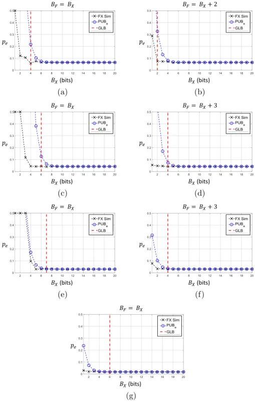
(bits) (a) (bits) (b) (bits) (c) (bits) (d) (bits) (e) (bits) (f) (bits) (g)
Figure 3.1: Results for classification on the Breast Cancer Dataset: classi-fication error rate pe in fixed-point simulations (FX Sim), analytical proba-bilistic upper bound (PUBe), geometric lower bound (GLB) for BX = BF and BX−BF determined by (2.6) for linear (a,b), NLIM (second order poly-nomial) (c,d), quadratic form (e,f), and NLOM (RBF) (g) classifiers. For the NLOM classifier, (2.6) dictates BX =BF.
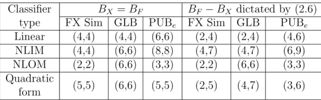
Table 3.1: Summary of Fig. 3.1 illustrating minimum precision requirements for hyperplane classifiers on the Breast Cancer Dataset dictated by FX Sim, GLB, and PUBe when BX =BF and BF −BX determined by (2.6).
Classifier type
BX =BF BF −BX dictated by (2.6) FX Sim GLB PUBe FX Sim GLB PUBe Linear (4,4) (4,4) (6,6) (2,4) (2,4) (4,6) NLIM (4,4) (6,6) (8,8) (4,7) (4,7) (6,9) NLOM (2,2) (6,6) (3,3) (2,2) (6,6) (3,3) Quadratic
form (5,5) (6,6) (5,5) (2,5) (4,7) (3,6)
except for the NLOM classifier which was trained using the commercial LIB-SVM package [30].
For the linear classifier, Fig. 3.1(a) shows the validity of the GLB and the PUBe for equal input and weight precisions. Indeed, fixed-point simulations for precisions larger than the GLB (4 bits) offer no significant accuracy gains while lower precisions seem to quickly degrade the accuracy. The PUBe also successfully upper bounds the error obtained in fixed-point. Figure 3.1(b) shows the benefits of using (2.6) which dictates in this example that
BF =BX + 2. Indeed, not only are the GLB and PUBe still valid, but it is also possible to decreaseBX to 2 bits, as reflected by the GLB and supported by the fixed-point simulation, while maintaining good accuracy.
Similar trends are observed for NLIM (Fig. 3.1(c,d)) and quadratic form (Fig. 3.1(e,f)) classifiers. Indeed, the GLB reaches the precision value after which the fixed-point accuracy saturates to within 2 bits, and the PUBe successfully upper bounds the fixed-point probability of error. Interestingly, the PUBe is much tighter for the quadratic form classifier as compared to the NLIM classifier.
Figure 3.1(g) shows our results for the NLOM classifier. There are a total of 98 support vectors. In this case (2.6) results in BX = BF, and this is why we have only one plot. Observe that the PUBe is much tighter than the GLB. Indeed, the PUBe tracks the fixed-point simulations to precisions as low as 3 bits. The GLB predicts 6 bits.
A detailed breakdown of the minimum precision requirements determined by FX Sim, GLB, and PUBe for all classifier types is presented in Table 3.1. So far, all results were performed on the Breast Cancer Dataset. To show the generality of our results, we also conduct a similar experiment on the ‘two
(bits) (a) (bits) (b)
Figure 3.2: Results for linear classification on the ‘two vs. four’ task for the MNIST Dataset: classification error rate pe in fixed-point simulations (FX Sim), analytical probabilistic upper bound (PUBe), geometric lower bound (GLB) for (a) BX =BF and (b)BX −BF = 6 as dictated by (2.6).
vs. four’ task on the MNIST Dataset where we consider a linear classifier. Again, the classifier is first pretrained using SGD as discussed in Section 1.2. The training and test sets were obtained by selecting the ‘two’ and ‘four’ instances from the original MNIST dataset. Overall, we had 11800 training and 2014 testing samples, respectively. The classifier was trained using SGD with γ = 2−10 and λ = 1. The results are shown in Fig. 3.2. Once again, we
find the numerical results to be consistent with the analysis of Section 2.1. Interestingly, in the experiments on the Breast Cancer Dataset, (2.6) seemed to always yield a BF larger than BX by a few bits (2 or 3) except for the case of NLOM. For the MNIST experiment, this trend seems to continue and is even more pronounced as the difference BF −BX = 6 bits. In fact, this should not be surprising. Indeed, the feature vectors in the MNIST dataset are grayscale images whereas the weights define the separating hyperplane. It is hence reasonable to expect the precision requirements of weights to be higher as slight changes to the separating hyperplane are more detrimental to the classification accuracy.
3.3
Complexity vs. Accuracy Trade-offs
We compare costs and performance for the following setups:1. minimum value of BX specified by the GLB with BX =BF,
BX and BF satisfying (2.6),
3. 8 bit quantization for all parameters,
4. an arbitrary precision assignment not satisfying the bounds presented in Section 2.1.
The first setup takes into account only one half of the theory proposed in Section 2.1, while the second shows the possibility and benefits of lever-aging both GLB and PUB for more aggressive, yet principled quantization. We chose 8 bits in the third setup as it is a typical representative of low-precision/high-performance arithmetic [22]. The fourth setup is intended to highlight the drawbacks of aggressive and unprincipled quantization.
For the Breast Cancer Dataset, Table 3.2 shows how our principled quan-tization strategy makes it possible to operate at low cost while maintaining accuracy. Indeed, for the linear classifier, an unstructured precision assign-ment of 2 and 3 bits for inputs and weights, respectively, does reduce the computational and representational costs, but results in a relatively high test error. At the expense of only ∼1.2× (178/146) computational cost and ∼ 1.2× representational cost, ∼ 1.8× classification error rate reduction is possible using a (2,4) quantization as dictated by (2.6) and the GB. This corresponds to ∼ 5× reduction in computational cost and ∼ 2.6× reduc-tion in representareduc-tional cost compared to the tradireduc-tional 8 bits quantizareduc-tion. Similar trends are observed for the other classifiers.
Similarly, this comparison for the MNIST experiment is shown in Table 3.3. Interestingly, we observe here that the constraint BX = BF is too harsh. Indeed, although the value BX = BF = 9 bits determined by the GLB yields a resulting accuracy ∼2× better than the precision assignment of BX =BF = 8 bits, this should not be considered a satisfactory result. In fact, when taking into account the trade-off betweenBX andBF as described in (2.6), BF = BX + 6 here, we are able to reduce BX down to only 4 bits. This corresponds to ∼1.7× and ∼ 1.3× decrease in the computational and representational costs with a negligible degradation in accuracy. Note that this quantization strategy results in a classifier∼2×more accurate than the one quantized to 8 bits in spite of using ∼2×10⁴ fewer F As and∼2×10³
fewer bits for data and weight representation. This highlights the importance of the analysis of the trade-off between input and weight precisions that was
Table 3.2: Results for the Breast Cancer Dataset. Comparison of compu-tational cost, represencompu-tational cost, and test error for linear, NLIM (second order polynomial), quadratic form, and NLOM (RBF) classifiers. The pre-cision assignments considered are the standard low prepre-cision quantization (8,8), the minimum (BX, BF) satisfying the GLB whenBX =BF, the mini-mum (BX, BF) satisfying the GLB whenBF −BX is dictated by (2.6), and one arbitrarily chosen assignment violating the bounds in Section 2.1. In the case of the NLOM classifier, the second and third precision assignments are identical. In each case, the use of the GLB and (2.6) makes it possible to reduce complexity but maintain accuracy.
Linear Classifier (BX, BF)
Computational cost (#F A)
Representational
cost (bits) Test error
(8,8) 894 168 6.6%
(4,4) 286 84 5.9%
(2,4) 178 64 7.5%
(2,3) 146 53 13.5%
NLIM (second order polynomial) Classifier (BX, BF)
Computational cost (#F A)
Representational
cost (bits) Test error
(8,8) 5.9×10³ 1048 4.4%
(6,6) 3.7×10³ 786 4.4%
(4,7) 3.1×10³ 722 4.0%
(3,3) 1.4×10³ 393 11.8%
Quadratic form Classifier (BX, BF)
Computational cost (#F A)
Representational
cost (bits) Test error
(8,8) 11.9×10³ 1048 3.2% (7,7) 9.5×10³ 917 3.2% (4,7) 5.6×10³ 887 3.0% (4,4) 3.8×10³ 524 9.8% NLOM (RBF) Classifier (BX, BF) Computational cost (#F A) Representational
cost (bits) Test error
(8,8) 10×104 7920 1.8%
(6,6) 6.6×10⁴ 5940 1.8%
Table 3.3: Results for linear classification on the ‘two vs. four’ task for the MNIST Dataset. Comparison of computational cost, representational cost, and test error. The precision assignments considered are the minimum (BX, BF) satisfying the GLB when BX = BF, the standard low precision quantization (8,8), the minimum (BX, BF) satisfying the GLB when BF −
BX = 6 as dictated by (2.6), one arbitrarily chosen assignment of (3,6) violating the bounds in Section 2.1. The use of the GLB and (2.6) makes it possible to reduce complexity but maintain accuracy.
(BX, BF)
Computational cost (#F A)
Representational
cost (bits) Test error (9,9) 85×103 14×103 2.3% (8,8) 70×103 13×103 4.4% (4,10) 49×103 11×103 2.2% (3,6) 28×103 7×10³ 8.5% described in Section 2.1.
3.4
Training Behavior
Here we illustrate the impact of precision on training as evidence to support the discussion in Section 2.2. We start with the Breast Cancer Dataset. The feedforward precisions are set as follows: we choose BX = 6 in order to separate the Theorem 3 scenario from the three boundary cases in Appendix 2.3.3, and we choose BF as specified by the GLB. That way, the feedforward precisions are minimal in a geometric sense and the full convergence of the algorithm is determined by the weight update precision (Theorem 3).
We shall consider a linear and a quadratic form classifier. We consider two scenarios: training with a small step size (γ = 2−10) and training with a large step size (γ = 2−5). The dataset is once again split into 500 training
and 500 testing samples. Each time we show the convergence behavior of the training loss function, which is the objective being minimized, and the test error rate, which is the target metric to be minimized. Each experiment is conducted over 30 independent runs and the curves shown hereafter are ensemble averages over these runs. For each run, the initial weights are set to zeros and λ is set to 1.
Figure 3.3 shows convergence curves for a linear classifier trained on the Breast Cancer Dataset. We show convergence curves for weight update
pre-(γ = 2−10) Iteration Index Tr ai ni ng L os s Func ti on (a) (γ = 2−10) Tes t Er ror R at e Iteration Index (b) (γ = 2−5) Iteration Index Tr ai ni ng L os s Func ti on (c) (γ = 2−5) Tes t Er ror R at e Iteration Index (d)
Figure 3.3: Results for linear classifier training on the Breast Cancer Dataset: (a) ensemble training loss function (1.6) and (b) ensemble test error rate for a small learning rate; (c) ensemble training loss function and (d) ensemble test error rate for a large learning rate. FL Sim denotes the floating-point simulation. In each case, a weight update precision of BX −log2(γ)
(Theo-rem 3) is enough to mimic floating-point behavior in fixed-point. Accuracy degradation is observed for lower precisions.
cisions of: (a)BX−log2(γ) (Theorem 3), 1−log2(γ) (Boundary Case 1), (b)
2−log2(γ) (Boundary Case 2), and −log2(γ) (Boundary Case 3). As shown, in both scenarios, a weight update precision of BX −log2(γ) is enough to
mimic floating-point behavior in fixed-point. For weight update precisions of 1−log2(γ) and −log2(γ), the occasional sign-SGD updates are not enough for convergence as discussed in Sections 2.2 and 2.3.3. For a weight update precision of 2−log2(γ), we do observe a decrease in the training loss func-tion and the test error rate, but the accuracies obtained are not as good as those of the floating-point trials. This demonstrates the sufficiency property of Theorem 3.
As far as the training loss function is concerned, similar trends are observed for the quadratic form (Fig. 3.4) classifier. Interestingly, the test error rate
(γ = 2−10) Tr ai ni ng L os s Func ti on Iteration Index (a) (γ = 2−10) Tes t Er ror R at e Iteration Index (b) (γ = 2−5) Tr ai ni ng L os s Func ti on Iteration Index (c) (γ = 2−5) Tes t Er ror R at e Iteration Index (d)
Figure 3.4: Results for quadratic form classifier training on the Breast Cancer Dataset: (a) ensemble training loss function ((1.6), matrix (Frobenius) norm replaces vector norm) and (b) ensemble test error rate for a small learning rate (γ = 2−10); (c) ensemble training loss function and (d) ensemble test error rate for a large learning rate (γ = 2−5). FL Sim denotes the
floating-point simulation. The weight update precision of 2BX −log2(γ) (Corollary
3.1) only marginally improves the accuracy over that of BX −log2(γ).
does go down in spite of imprecise updates. Nonetheless, we see that higher precision leads to greater overall accuracy. Note that we not only considered weight update precision of BX−log2(γ), but also 2BX −log2(γ) as dictated
by Corollary 3.1. Results show that this increased precision only marginally improves the convergence behavior.
Figure 3.5 illustrates these results for the ‘two vs. four’ classification task on the MNIST Dataset for linear classification with a learning rate of 2−10.
The feedforward precisions are again chosen to be minimal in the geomet-ric sense. Those precisions were determined in the previous subsection to be 4 and 10 for the inputs and weights, respectively. The results here are very consistent with those observed for the experiments on the Breast Can-cer Dataset. Indeed, it is clearly seen that a weight update precision of
(γ = 2−10) Iteration Index Tr ai ni ng L os s Func ti on (a) (γ = 2−10) Tes t Er ror R at e Iteration Index (b)
Figure 3.5: Results for linear classifier training on the ‘two vs. four’ task for the MNIST Dataset: (a) ensemble training loss function (1.6) and (b) ensemble test error rate for a learning rate γ = 2−10. FL Sim denotes the
floating-point simulation. A weight update precision of BX −log2(γ)
(The-orem 3) is enough to mimic floating-point behavior in fixed-point. Accuracy degradation is observed for lower precisions.
BW = BX −log2(γ) as dictated by Theorem 3 is of paramount importance
for successful convergence. The results here are very consistent with those observed for the experiments on the Breast Cancer Dataset. Indeed, it is clearly seen that a weight update precision of BW = BX −log2(γ) as
dic-tated by Theorem 3 is of paramount importance for successful convergence.
3.5
Summary
In this chapter we have validated the theoretical results presented in Chap-ter 2. We have presented fixed-point simulations on the Breast Cancer and MNIST datasets. The numerical results show close agreement with the pre-dicted precision requirements. Furthermore, the benefits of the analysis in terms of complexity reduction have been illustrated. New complexity metrics have been proposed in the computational and representational costs. These two meaningful costs, as well as the presented precision analysis, provide a natural way for designers to estimate complexity measures in fixed-point and to better explore the trade-offs of accuracy vs. precision and complexity.
CHAPTER 4
CONCLUSION
We have presented a theoretical analysis of the behavior of general fixed-point margin hyperplane classifiers. The results presented consist of bounds based on the geometry and statistics of the classification task and on the conver-gence conditions of the training task. By characterizing the trade-off between input and weight precisions, an efficient precision reduction scheme was pre-sented. This framework eliminates the need for expensive trial-and-error. Furthermore, it presents guidelines for minimizing resource utilization. This utilization was captured by the computational and representational costs. Simulation results shown support the developed theory and highlight its ben-efits.
Several insights can be taken from our work. These include a trade-off between input and weight precision which is useful for minimizing the over-all precision. Furthermore, it was observed from the GLB that precision increases logarithmically with the dimensionality of the problem. From the PUB, it was seen that the mismatch probability between fixed-point and floating-point classifier decays, at worst, exponentially with precision. It is in fact possible to derive a tighter bound on this mismatch probability us-ing the Chernoff bound which marginally improves this dependence makus-ing it double exponential in precision. Finally, it was shown that the early stopping criterion applies to fixed-point training and provides a sufficient condition on the weight update precision for full convergence.
Future work includes a deeper dive into the topic of complexity vs. accu-racy in machine learning. This includes a similar analysis for more compli-cated algorithms such as deep neural networks. The presented work takes a conservative approach in the model of quantization. It is possible to shape quantization noise statistics using dithering during training. Such an ap-proach might lead to greater reductions in precision. Another line of work is to study the effects of floating-point quantization. While fixed-point
im-plementations are usually more efficient than floating-point ones, the latter benefit from a much wider dynamic range which could be beneficial to the ro-bustness in classification. An orthogonal direction is to consider the structure of the algorithms themselves. It is well established that data-driven models inhibit large redundancies which can be exploited to trade off complexity with robustness. The above constitute the first steps in the important task of developing a unified and principled framework to understand complexity vs. accuracy in the design and implementation of machine learning systems.
REFERENCES
[1] A. Coates et al., “Deep learning with COTS HPC systems,” in Proceed-ings of the 30th International Conference on Machine Learning, 2013, pp. 1337–1345.
[2] S. Gupta et al., “Deep Learning with Limited Numerical Precision,” in Proceedings of The 32nd International Conference on Machine Learning, 2015, pp. 1737–1746.
[3] M. Kim et al., “Bitwise Neural Networks,” arXiv preprint arXiv:1601.06071, 2016.
[4] M. Courbariaux et al., “Binaryconnect: Training deep neural networks with binary weights during propagations,” in Advances in Neural Infor-mation Processing Systems, 2015, pp. 3123–3131.
[5] M. Courbariaux et al., “Binarynet: Training deep neural networks with weights and activations constrained to+ 1 or-1,” arXiv preprint arXiv:1602.02830, 2016.
[6] M. Rastegari et al., “XNOR-Net: ImageNet Classification Using Bi-nary Convolutional Neural Networks,”arXiv preprint arXiv:1603.05279, 2016.
[7] D. Lin et al., “Fixed Point Quantization of Deep Convolutional Net-works,” arXiv preprint arXiv:1511.06393, 2015.
[8] D. Lin et al., “Overcoming challenges in fixed point training of deep convolutional networks,” arXiv preprint arXiv:1607.02241, 2016. [9] M. Goel et al., “Finite-precision analysis of the pipelined
strength-reduced adaptive filter,” Signal Processing, IEEE Transactions on, vol. 46, no. 6, pp. 1763–1769, 1998.
[10] C. Caraiscos and B. Liu, “A roundoff error analysis of the lms adap-tive algorithm,” IEEE Transactions on Acoustics, Speech, and Signal Processing, vol. 32, no. 1, pp. 34–41, 1984.
[11] W. Sung and K.-I. Kum, “Simulation-based word-length optimization method for fixed-point digital signal processing systems,” IEEE Trans-actions on Signal Processing, vol. 43, no. 12, pp. 3087–3090, 1995. [12] R. Rocher et al., “Accuracy evaluation of fixed-point LMS
algo-rithm,” in Acoustics, Speech, and Signal Processing, 2004. Proceed-ings.(ICASSP’04). IEEE International Conference on, vol. 5. IEEE, 2004, pp. V–237.
[13] C. Shi and R. W. Brodersen, “An automated floating-point to fixed-point conversion methodology,” in Acoustics, Speech, and Signal Pro-cessing, 2003. Proceedings.(ICASSP’03). 2003 IEEE International Con-ference on, vol. 2. IEEE, 2003, pp. II–529.
[14] R. Gupta and A. O. Hero, “Transient behavior of fixed point LMS adap-tation,” in Acoustics, Speech, and Signal Processing, 2000. ICASSP’00. Proceedings. 2000 IEEE International Conference on, vol. 1. IEEE, 2000, pp. 376–379.
[15] P. S. Diniz et al., “Analysis of LMS-Newton adaptive filtering algo-rithms with variable convergence factor,” IEEE Transactions on Signal Processing, vol. 43, no. 3, pp. 617–627, 1995.
[16] C. Cortes and V. Vapnik, “Support-vector networks,” Machine Learn-ing, vol. 20, no. 3, pp. 273–297, 1995.
[17] K. H. Lee et al., “Low-energy formulations of support vector machine kernel functions for biomedical sensor applications,” Journal of Signal Processing Systems, vol. 69, no. 3, pp. 339–349, 2012.
[18] L. Bottou, “Large-scale machine learning with stochastic gradient de-scent,” in Proceedings of COMPSTAT’2010. Springer, 2010, pp. 177– 186.
[19] C. Sakr et al., “Minimum precision requirements for the SVM-SGD learning algorithm,” in Acoustics, Speech and Signal Processing (ICASSP), 2017 IEEE International Conference on. IEEE, 2017. [20] Y. Chen et al., “Eyeriss: An energy-efficient reconfigurable accelerator
for deep convolutional neural networks,” in 2016 IEEE International Solid-State Circuits Conference (ISSCC). IEEE, 2016, pp. 262–263. [21] D. Liu, T. Chen, S. Liu, J. Zhou, S. Zhou, O. Teman, X. Feng, X. Zhou,
and Y. Chen, “Pudiannao: A polyvalent machine learning accelerator,” inACM SIGARCH Computer Architecture News, vol. 43, no. 1. ACM, 2015, pp. 369–381.
[22] M. Abadi et al., “Tensorflow: A system for large-scale machine learning,” Google Brain, Tech. Rep., 2016, arXiv preprint. [Online]. Available: https://arxiv.org/abs/1605.08695
[23] B. Widrow and I. Koll´ar, Quantization Noise. Cambridge University Press, 2008, vol. 2.
[24] B. Liu and T. Kaneko, “Error analysis of digital filters realized with floating-point arithmetic,” Proceedings of the IEEE, vol. 57, no. 10, pp. 1735–1747, 1969.
[25] E. H. Lee, D. Miyashita, E. Chai, B. Murmann, and S. S. Wong, “Lognet: Energy-efficient neural networks using logarithmic computa-tion,” in Acoustics, Speech and Signal Processing (ICASSP), 2017 IEEE International Conference on. IEEE, 2017, pp. 5900–5904.
[26] C. Zhu, S. Han, H. Mao, and W. J. Dally, “Trained ternary quantiza-tion,” arXiv preprint arXiv:1612.01064, 2016.
[27] C. Sakr et al., “Analytical Guarantees on Numerical Precision of Deep Neural Networks,” in International Conference on Machine Learning, 2017, pp. 3007–3016.
[28] A. Asuncion et al., “UCI machine learning repository,” 2007.
[29] Y. LeCun et al., “The mnist database of handwritten digits,” 1998. [30] C.-C. Chang et al., “LIBSVM: a library for support vector machines,”
ACM Transactions on Intelligent Systems and Technology (TIST), vol. 2, no. 3, p. 27, 2011.