Agarwal, A., Juneja, S. and Sircar, R. (2016) American options under stochastic
volatility: control variates, maturity randomization & multiscale asymptotics.
Quantitative Finance, 16(1), pp. 17-30.
There may be differences between this version and the published version. You are
advised to consult the publisher’s version if you wish to cite from it.
http://eprints.gla.ac.uk/147370/
Deposited on: 6 September 2017
Enlighten – Research publications by members of the University of Glasgow
http://eprints.gla.ac.uk
American Options under Stochastic Volatility: Control
Variates, Maturity Randomization & Multiscale Asymptotics
Ankush Agarwal∗ Sandeep Juneja † Ronnie Sircar‡ June 28, 2015
Abstract
American options are actively traded worldwide on exchanges, thus making their accurate and efficient pricing an important problem. As most financial markets exhibit randomly varying volatility, in this paper we introduce an approximation of American option price under stochastic volatility models. We achieve this by using the maturity randomization method known as Canadization. The volatility process is characterized by fast and slow scale fluctuating factors. In particular, we study the case of an American put with a single underlying asset and use perturbative expansion techniques to approximate its price as well as the optimal exercise boundary up to the first order. We then use the approximate optimal exercise boundary formula to price American put via Monte Carlo. We also develop efficient control variates for our simulation method using martingales resulting from the approximate price formula. A numerical study is conducted to demonstrate that the proposed method performs better than the least squares regression method popular in the financial industry, in typical settings where values of the scaling parameters are small. Further, it is empirically observed that in the regimes where scaling parameter value is equal to unity, fast and slow scale approximations are equally accurate.
Keywords and phrases. Stochastic volatility, American option, maturity randomization, singular perturbation theory, regular perturbation theory, Monte Carlo, control variate
AMS subject classification. 91G60, 91G80, 60H30
JEL subject classification. G13
∗
School of Technology and Computer Science, Tata Institute of Fundamental Research, Mumbai 400005;
[email protected]. Work partially supported by Tata Consultancy Services Ph.D. scholarship.
†
School of Technology and Computer Science, Tata Institute of Fundamental Research, Mumbai 400005;
‡
ORFE Department, Sherrerd Hall, Princeton University, Princeton NJ 08544;[email protected]. Work partially supported by NSF grant DMS-1211906.
1
Introduction
In this paper, we develop approximations for the optimal exercise boundary and price of Ameri-can options under stochastic volatility, where the volatility process is modulated by fluctuations occurring on fast or slow time scales. We particularly consider the example of an American put with a single underlying asset. It is also made clear that the case of an American call option written on a dividend-paying underlying asset can be handled similarly. In order to derive these approximations, we replace the fixed maturity of the option with an exponentially distributed random variable to introduce an American put with random maturity. We then use singular and regular perturbation techniques to approximately solve the pricing problem associated with the random maturity American put. We demonstrate, with the help of numerical experiments, that the resulting approximation of the optimal exercise boundary for this new put can be used to estimate the price of original option with fixed maturity via Monte Carlo. Moreover, we use the approximation of the random maturity put price to form efficient martingale control variates for our simulation method.
In the classical theory of risk-neutral pricing, the price of an American option corresponds to the solution of an optimal stopping problem which, in Markovian models, can also be expressed as a free boundary problem. Even in the simple case of constant volatility, the American option price is not available in closed form. Over the years, many numerical and simulation techniques have been developed to approximately solve either of the two formulations for American option pricing problem. The prominent numerical methods in the constant volatility case are the binomial lattice method of Cox et al. [10], and the approximation method proposed by Brennan and Schwartz [6] where the associated free boundary problem is solved numerically such that the boundary conditions are not violated. Carr [9] introduced the maturity randomization technique where fixed maturity of the American put is successively replaced by random variables corresponding to the arrival times of an independent Poisson process. The partial differential equation (PDE) satisfied by the price of this transformed option becomes similar to the pricing PDE of a perpetual American put, which can be solved explicitly for every instance of maturity randomization. The series of these solutions is then used to approximate the price of original American put. Bouchard et al. [5] proved that the approximation of American put value obtained via maturity randomization converges to the true value with successive randomization iteration of the algorithm. This so-called Canadization method is also extended recently for optimal multiple stopping problems in Lévy models by Leung et al. [22]. Other examples of application of the Canalization method to price American and Russian options are [21], [11], [20].
In order to estimate the true American option value, simulation methods typically solve the discretized version of the option pricing problem, where exercise can happen only at a finite number of fixed times. As the number of exercise opportunities increases to infinity, the price of this discrete exercise American option converges to the true value. In this setting, simulation methods approximately solve the dynamic program associated with the pricing problem. To facilitate this, first, the so-called continuation value function is estimated at each exercise op-portunity using simulated underlying sample paths via Monte Carlo, and then, based on these estimates, an approximately optimal exercise policy is defined. This policy is used to exercise on the simulated sample paths, and the average payoff on these exercised sample paths is used as an estimator for the true American option price. The random tree method of Broadie and Glasserman [7] used nested paths simulation to estimate the continuation value function. In the stochastic mesh method, Broadie and Glasserman [8] used a likelihood ratio weighted average on simulated sample paths to estimate the continuation value recursively. These methods were limited in their success due to their slow convergence rate for a given computational budget. In 2001, Longstaff and Schwartz [23] proposed the least squares regression method where the
continuation value function is modeled as a linear combination of pre-specified basis functions in the L2–space. This method has proven to be very popular in practice due to its fast rate of convergence, and it is considered as a benchmark in simulation methods for American option pricing. Recently, an improvement of Longstaff-Schwartz method has been proposed by Gra-macy and Ludkovski [15] where the authors adaptively learn the classifiers which are then used in dynamic regression algorithms to estimate the option value function.
Empirical evidence in many studies (see Rubinstein [25]) shows that the implied volatility of options exhibit a smile curve (or skew). In order to capture this phenomenon, stochastic volatility models were proposed (see e.g., Hull and White [17] and Heston [16]). A common theme in all the proposed stochastic volatility models is mean-reversion of a stochastic factor driving the volatility of the underlying process. A detailed discussion of the mean-reverting nature of these models is provided by Fouque et al. [13] where empirical references are given for fast and slow factors in volatility fluctuations. Hence, in [13], the authors proposed multiscale stochastic volatility models which capture both the separation of scales and mean-reverting characteristics of the volatility process.
The problem of pricing European options in the stochastic volatility setting has been well studied. In the Heston model, the European option price appears as a Fourier inversion inte-gral which can be efficiently calculated using numerical methods. Fouque et al. [13] provide an approximation for European option prices for calibration in the multiscale model which is reasonably accurate. Relatively, little has been done to address the problem of American option pricing in stochastic volatility setting. The few existing methods in the literature can be broadly categorized as PDE and non-PDE based methods. The PDE based methods provide an approx-imation for the price of American option by numerically solving the (at least three-dimensional) free boundary problem. A popular approach is to solve the problem by reformulating it as a lin-ear complementarity problem. In order to solve each discrete complementarity problem, Ikonen and Toivanen use operator splitting methods in [18], and use component-wise splitting methods in [19]. These methods are time-consuming and are typically dependent on sophisticated solver packages. In non-PDE methods, a variant of the Longstaff-Schwartz method with cross-sectional basis functions can be used for pricing as demonstrated by Rambharat and Brockwell [24].
As mentioned earlier, in our work, we develop an approximation for the finite time-horizon American put price and the associated optimal exercise boundary under stochastic volatility. We use the idea of maturity randomization proposed by Carr [9] to reduce the original pricing PDE to a pricing PDE problem corresponding to a perpetual American put. We use perturbation theory and variation of parameters techniques to approximate the put price and the optimal exercise boundary. The optimal boundary approximation is used to exercise simulated underlying paths and estimate the true American option price. We compare the performance of our method with an implementation of the Longstaff-Schwartz method as suggested in [24] and demonstrate better numerical accuracy under typical parameter settings and small computational budget. Fouque and Han [12] provided centered martingales which can be possibly used as control variates for estimating the true option price. However, the true option price function appears in these centered martingales. We replace the true option price function with our approximate price function and use the resulting martingales to form control variates for our simulation method. The proposed control variates lead to a considerable variance reduction in the case of fast mean-reverting stochastic volatility as shown in the numerical examples. In our numerical experiments, we also observe that in the regime where value of scaling parameter is equal to one, fast and slow scale approximations are equally accurate.
For simplicity of presentation, we analyze the two stochastic volatility factors separately. In Section 2 we consider the case of fast mean-reverting volatility process which leads to a singular perturbation problem for the associated pricing PDE. It is evident from the calculations that
one does not require to track the fast mean-reverting volatility level to calculate the put price approximation. Next, in Section 3, we derive the approximation for American put price and optimal exercise boundary in the case of slowly fluctuating volatility. In Sections 2.2 and 3.2, we show how to use the price and boundary approximations to form effective control variates using the fast and slow factor approximations respectively. A detailed numerical study comparing our method with the Longstaff-Schwartz method is presented in Section 4. We conclude with few comments on our work and some suggestions for further research in Section 5. The proofs are relegated to Appendix A. We explain the numerical implementation of the respective fast and slow scale control variates in Appendix B.
2
Approximation under fast mean-reverting stochastic volatility
We first consider a fast mean-reverting stochastic volatility model. Here, letX denote the price of a non-dividend paying asset whose dynamics under the risk-neutral probability measure Pis
given by the following system of SDEs:
dXt=rXtdt+f(Yt)XtdWt(1), X0 =x >0, (1) dYt= 1 ε(m1−Yt)dt+ν1 r 2 εdW (2) t , Y0 =y, (2)
whereWt(1) andWt(2) are one-dimensional Brownian motions with correlationdhW(1), W(2)it=
ρ1dt, ρ21 < 1 and ε > 0 is the intrinsic time-scale of Y. We choose specific form of the drift
function: (m1−Yt)and volatility function: √
2ν1such thatY is an ergodic process (the
Ornstein-Uhlenbeck process) with unique invariant distribution denoted byΦwhich is normalN(m1, ν12)
and does not depend onε.Further, we requiref :R→R+\{0}to be a continuously differentiable
function such thatR f2(y)Φ(y)dy <∞.We assumeε <<1so that the intrinsic time-scale of Y
is small and hence it represents a fast mean-reverting stochastic factor of underlying volatility. Under the risk-neutral probability measure, the price at time t < T of an American put option with maturityT <∞ is
Pε(t,x,˜ y˜) := sup τ∈T[t,T]Et,x,˜˜y h e−r(τ−t)(K−Xτ)+ i , (3)
whereK is the strike price, andT[t,T] is the set of stopping timesτ taking values in[t, T]. It can be shown, using the dynamic programming principle, that the American put value is the solution of a free boundary problem. The standard approach to solve this problem is to separate the space of state variables into two regions, the hold- and exercise- region where the boundary of the region is regarded as the optimal exercise boundary. However, it is not possible to calculate an explicit solution for the free boundary problem.
In order to solve this problem approximately, we randomize the maturity of the American put and replace it with an exponentially distributed independent random variableτλwith mean
1
λ = T. Following the arguments in Carr [9], we can write the price of American put with
random maturity as follows
P(1)(x, y) := sup τ∈T[0,∞] Ex,y h e−r(τ∧τλ)(K−X τ∧τλ) +i.
As the option maturity is an exponentially distributed random variable, by the memoryless property, the option gets no closer to its random maturity as the time elapses and thus its value suffers no time decay. As the exercise value is also time stationary, the exercise boundary
becomes time-independent as well and we need to search for a single critical stock price which depends on the level of stochastic volatility factor. Thus, we look for the optimal exercise boundary parametrized byy.
For the proposed multiscale stochastic volatility model, it is clear that the smooth pasting condition forP(1)(x, y)holds w.r.t.(x, y) from Lemma 2.1 in [28]. Thus, we look for a solution that satisfies the following PDE in the hold region with the smooth pasting conditions:
LεP(1)(x, y) +λ(K−x)+ = 0, for x > xb(y), (4) P(1)(xb(y), y) =K−xb(y), ∂P(1) ∂x (xb(y), y) =−1, ∂P(1) ∂y (xb(y), y) = 0,
wherexb(y)is the optimal exercise boundary. Here, the operatorLε is given by:
Lε= 1 εL0+ 1 √ εL1+L2, where we define L0 :=ν12 ∂2 ∂y2+(m1−y) ∂ ∂y, L1 := √ 2ρ1ν1xf(y) ∂2 ∂x∂y, L2 := 1 2f 2(y)x2 ∂2 ∂x2+rx ∂ ∂x−(r+λ)·.
Note that L0 is the infinitesimal generator of an OU process with unit rate of mean reversion. In the exercise region, we have
P(1)(x, y) =K−x, for x < xb(y). (5)
For a general stochastic volatility functionf(y), there is no analytic solution to the free-boundary problem (4)-(5). In the limit ε & 0, this is a singular perturbation problem and thus our approach is to construct an asymptotic approximation.
2.1 Asymptotic analysis
Specifically, we perform a singular perturbation with respect to the small parameterε, expanding the solution and exercise boundary in powers of√ε
P(1)(x, y) =P0(x, y) + √ εP1(x, y) +εP2(x, y) +· · · , (6) xb(y) =x0(y) + √ εx1(y) +· · ·. (7)
This particular choice of expansion in powers of √εallows us to analytically solve for terms in the expansion, independent of ε. We now plug (6) and (7) into (4) - (5), and collect terms of equal powers of√ε. For x > xb(y),we get
1 εL0P0+ 1 √ ε(L0P1+L1P0) + L0P2+L1P1+L2P0+λ(K−x) + +√ε(L0P3+L1P2+L2P1) +· · ·= 0, (8)
where we have suppressed the dependence on(x, y) for notational convenience. For x < xb(y),
in (5), we use the asymptotic expansion of (7) in the right hand side and use (6) in the left hand side to perform a Taylor series expansion aroundx0(y) to write
P0(x0(y), y) + √ ε x1(y) ∂P0 ∂x x 0(y) +P1(x0(y), y) +· · ·=K−x0(y)− √ εx1(y) +· · ·. (9)
Similarly, the boundary conditions can be expanded as ∂P0 ∂x x 0(y) +√ε x1(y) ∂2P0 ∂x2 x 0(y) +∂P1 ∂x x 0(y) +· · ·=−1, (10) ∂P0 ∂y x0(y) +√ε x1(y) ∂2P0 ∂y∂x x0(y) +∂P1 ∂y x0(y) +· · ·= 0.
Zeroth order terms. Collecting terms of order1/ε in (8) and order1 in (9) and (10), we have the following PDE and boundary condition:
L0P0(x, y) = 0, for x > x0(y), P0(x, y) =K−x, for x≤x0(y), ∂P0 ∂x x0(y) =−1.
AsL0 is the infinitesimal generator ofY, zero is an eigenvalue with constant as its eigenfunction.
Thus, the first equation implies that we may seek P0 of the form P0 =P0(x). Along with the
second equation above, it is easy to see that P0 is independent of y everywhere. As P0 is
independent of y on either side of the exercise boundary x0(y), we can conclude thatx0 is also
independent of y. We make use of this observation going forward.
First order terms. Collecting terms of order 1/√ε in (8) and order √ε in (9) and (10) leads to the following PDE and boundary condition:
L0P1(x, y) = 0, forx > x0, P1(x, y) = 0, forx≤x0, x1(y) ∂2P 0 ∂x2 x0 +∂P1 ∂x x0 = 0, (11)
where we have used the result that P0 is independent of y. As with P0, we can also takeP1 to
be independent of y. Thus, we can see that x1 is also independent of y.
Second order terms. Matching terms of order 1 in (8) and orderεin (9) leads to
L0P2+L2P0+λ(K−x)+= 0, for x > x0, (12)
P2(x, y) = 0, for x≤x0,
where we have used that P1 does not depend on y. The first equation is a Poisson equation for
P2with respect to the infinitesimal generatorL0with the source termL2P0+λ(K−x)+. A
well-behaved solution (polynomial growth at infinity) forP2 exists if and only ifL2P0+λ(K−x)+is
centered with respect to the invariant distribution of the diffusion whose infinitesimal generator isL0. Thus, the centering condition becomes
hL2P0i+λ(K−x)+= 0, (13)
where the angled brackets indicate taking the average of the argument with respect to Φ, the invariant distribution of Y. Since P0 does not depend on y, the centering condition becomes hL2iP0+λ(K−x)+ = 0which is equivalent to the ODE
1 2σ¯ 2x2d2P0 dx2 +rx dP0 dx −(r+λ)P0+λ(K−x) += 0,
where σ¯2 := hf2i = R f2(y)Φ(dy). The solution to the above ODE can be obtained from the calculations performed in [9].
Proposition 1. In the stochastic volatility model (1)–(2), the zeroth order approximation of randomized maturity American put price is given by
P0(x) = a01 Kx β1 +a02 xx0 β1 if x > K, b01 Kx β2 +a02 xx0 β1 +KR−x if x0 < x≤K, K−x if x≤x0, (14)
where the constants are γ = 1 2 − r ¯ σ2, R= λ λ+r, ∆ = r γ2+ 2λ Rσ¯2, p= ∆−γ 2∆ , q= 1−p, pˆ= ∆−γ+ 1 2∆ , ˆ q= 1−p,ˆ a01= (qKR−qKˆ ), a02=qKR r λ, b01= (ˆpK−pKR), β1=γ−∆, β2 =γ+ ∆.
The zeroth order approximation to the exercise boundary is given by
x0 =K pRr λ(ˆp−Rp) 1 β2 .
By plugging the expressions back in the above mentioned formulas, it can be easily verified thatx0≤K and P0(x) is continuous atK and x0.From (12), we have
L0P2 =−L2P0−λ(K−x)+=−(L2P0− hL2P0i),
which follows from (13). Therefore,
P2 =−
1
2(φ(y) + ˜c(x))x
2∂2P0
∂x2 , (15)
where function φsolves L0φ=f2(y)−¯σ2 and ˜c(x) is an arbitrary finite-valued function
inde-pendent of y.
Third order terms. Collecting terms of order √ε in (8) and order ε3/2 in (9), we obtain the following PDE and boundary condition:
L0P3+L1P2+L2P1= 0 for x > x0.
This is a Poisson equation iny forP3(x, y), which imposes a solvability condition on the source
term L1P2+L2P1, leading to
hL2iP1=−hL1P2i. (16)
We introduce a new convenient notation for the correction term P˜1 := √
εP1. Thus, plugging
P2, given by (15), into (16) gives:
hL2iP˜1 =V3 2x2∂ 2P 0 ∂x2 +x 3∂3P0 ∂x3 , (17) whereV3 := pε 2ρνhf(y)φ
0(y)i.The above ordinary differential equation can be solved to obtain
Proposition 2. The correction term P˜1 in the price expansion is given by ˜ P1(x) = ˆ a1 x x0 β1 −V3β12(β1−1) ¯ σ2∆ log(x) a01 x K β1 +a02 x x0 β1 if x > K, ˆ a2 x x0 β1 + ˆa3 x K β2 +V3log(x) ¯ σ2∆ h b01β22(β2−1) x K β2 −a02β12(β1−1) x x0 β1i if x0 < x≤K, 0 if x≤x0, where ˆ a1 = V3 2∆2σ¯2 a01β12(β1−1) +b01β22(β2−1) x0 K β2− x0 K β1 + V3 ∆¯σ2 β21(β1−1) a01( x0 K) β1log(K) +a 02log(x0) −b01 x0 K β2 β22(β2−1) log(x0/K) , ˆ a2 = V3 2∆2σ¯2 x0 K β2 a01β21(β1−1) +b01β22(β2−1)(1 + 2∆ log(K)) +V3log(x0) ∆¯σ2 a02β12(β1−1)−b01β22(β2−1) x0 K β2 , ˆ a3 =− V3 2∆2¯σ2 a01β21(β1−1) +b01β22(β2−1)(1 + 2∆ log(K)) . Let x˜1 := √
εx1.Then, the correction term in the optimal exercise boundary expansion is given
by ˜ x1=− dP˜1 dx x0 .d2P0 dx2 x0 where dP˜1 dx x0 = ˆa2β1 x0 +ˆa3β2 K x0 K β2−1 + V3 ¯ σ2∆ hb01β2 2(β2−1) K x K β2−1 (1 +β2logx0) + a02β12(β1−1) x0 (1 +β1logx0) i , d2P0 dx2 x0 = b01β2(β2−1) K2 x0 K β2−2 +a02β1(β1−1) x20 .
Remark 1. Ting et al. [27] performed a similar analysis as in Proposition 2, but for the case of a perpetual American option i.e. λ= 0, under fast-mean reverting stochastic volatility.
In the constant volatility case, Carr [9] used successive jump times of an independent Poisson process to randomize the maturity of American put in order to closely approximate the true American put price. In this work, we use an independent exponential random variable, which corresponds to the first jump time of an independent Poisson process, to randomize the maturity of the American put. Therefore, the obtained price approximationP0+
√
εP1may not be accurate
enough to approximate the true American put pricePε.The approximation can be improved by replacing the fixed maturity with successively increasing arrival times of an independent Poisson process as in Carr [9]. In this approach, the number of different coefficient calculations in the approximation terms increases with the number of boundary conditions and poses a significant computational challenge. This direction has been reserved for future research.
However, it has been empirically observed and theoretically proved (cf. Andersen [2], Be-lomestny [4], Agarwal and Juneja [1]) that simulation methods based on even a crude approxi-mation of the optimal exercise boundary produce good estimates for the true American option price. Thus, in Section 2.2, we use the exercise boundary approximationx0+
√
εx1in our setting
Remark 2. American call options on a dividend paying underlying can also be priced using the proposed methodology under the multiscale stochastic volatility model. In the case of an underlying with continuous dividend yield, we can use the American option put-call parity from Corollary 1 [26] to transform the original American call option pricing problem to an American put option pricing problem. It can be further checked that the free boundary problem for the new American put problem can be solved using the maturity randomization technique as in Section 2. Finally, to incorporate the discrete cash dividends, a correction to the exercise boundary condition can be introduced based on Equation (37) of [9].
2.2 Control variate for finite maturity American option pricing
Here we discuss how to form control variates for our simulation method to price an American put with finite maturity T under fast mean-reverting stochastic volatility. Let τ∗ denote the optimal stopping time in (3). As in [12], by applying Itô’s Lemma, we can write
Pε(0, x, y) :=e−rτ∗(K−Xτ∗)+− U0(Pε)−√1
εU1(P
ε),
whereU0 andU1 are defined as
U0(Pε) := Z τ∗ 0 e−rs∂P ε ∂x (s, Xs, Ys)f(Ys)XsdW (1) s , U1(Pε) := Z τ∗ 0 e−rs∂P ε ∂y (s, Xs, Ys) √ 2ν1dWs(2).
As an explicit formula forPεis not available, we use the approximation of the priceP(1)of the random maturity American put as given in Propositions 1 and 2 to calculate an approximation for the martingalesU0 andU1.Since, the terms P0 andP1 in the approximation are independent
of y, we only need to approximate U0(Pε) which is done by using
ˆ U0(P(1);xb) := Z τˆ 0 e−rs ∂ ∂x(P0+ √ εP1)(Xs)f(Ys)XsdWs(1),
where ˆτ is an approximation to optimal stopping time τ∗ defined using the optimal exercise boundary approximation x0+ √ εx1: ˆ τ := inf{t:Xt≤x0+ √ εx1} ∧T,
wherex0 andx1 are constants independent ofy.Hence, for a set ofN independent sample paths
of the underlying process X, a Monte Carlo estimator with the martingale control variate is given by 1 N N X i=1 h e−rτˆ(K−Xτ(ˆi))+−Uˆ0(i)(P(1);xb) i , (18)
where Xτˆ(i) is the value of theith underlying process sample path at τˆ. We provide details of the numerical implementation of control variates in Appendix B.
3
Slow scale volatility approximations
We conduct a similar analysis for the case when stochastic volatility is slowly fluctuating. Note that we do not require ergodicity of the slow scale factor Z. However, for simplicity of pre-sentation, we assume a specific form of the drift and volatility functions: (m2−Zt) and
√
respectively for the volatility driving processZ. In this case, the dynamics ofX is given by the following system of SDEs:
dXt=rXtdt+f(Zt)XtdWt(1), X0 =x >0,
dZt=δ(m2−Zt)dt+ν2 √
2δ dWt(3), Z0 =z,
whereWt(1) andWt(3) are one-dimensional Brownian motions with correlationdhW(1), W(3)it=
ρ2dt, ρ22 < 1 and 1/δ > 0 is the intrinsic time-scale of Z. We assume δ << 1 so that the
intrinsic time-scale of Z is large and hence it represents a slowly fluctuating stochastic factor of underlying volatility. Here, we require f : R → R+\{0} to be a continuously differentiable
function.
The price at time tof an American put option with maturityT <∞is
Pδ(t,x,˜ z˜) := sup τ∈T[t,T] Et,x,˜˜z h e−r(τ−t)(K−Xτ)+ i , (19)
whereK is the strike price, andT[t,T] is the set of stopping times τ taking values in [t, T]. The price of American put with independent exponentially distributed random maturity τλ, with
mean λ1 =T, is P(1)(x, z) := sup τ∈T[0,∞] Ex,z h e−r(τ∧τλ)(K−X τ∧τλ) +i.
Let us denote by xb(z) the optimal exercise boundary for American option with randomized
maturity defined above. Again, we look for a solutionP(1)(x, z)that satisfies the following PDE
in the hold region with the boundary conditions and smooth pasting conditions:
LδP(1)(x, z) +λ(K−x)+= 0, for x > xb(z), (20) P(1)(xb(z), z) =K−xb(z), ∂P(1) ∂x (xb(z), z) =−1, ∂P(1) ∂z (xb(z), z) = 0,
where the operator Lδ:=L 2+ √ δM1+δM2, with L2:= 1 2f 2(z)x2 ∂2 ∂x2 +rx ∂ ∂x−(r+λ)·, M1:= √ 2ρ2ν2f(z)x ∂2 ∂x∂z, M2 :=ν 2 2 ∂2 ∂z2 + (m2−z) ∂ ∂z.
In the exercise region, we have
P(1)(x, z) =K−x, for x < xb(z). (21)
In the limit δ & 0, the above problem is a regular perturbation problem and we look for an asymptotic approximation.
3.1 Asymptotic analysis
We expand P(1)(x, z)and the optimal exercise boundary xb(z) in powers of √ δ as follows P(1)(x, z) = P0(x, z) + √ δP1(x, z) +δP2(x, z) +· · · , xb(z) = x0(z) + √ δx1(z) +· · · .
We plug the asymptotic expansion formulas and repeat the procedure as followed in Section 2.1. Matching terms of order 1 (with respect to √δ) in (20)-(21) leads to the following PDE and boundary condition: L2P0+λ(K−x)+= 0, for x > x0(z), (22) P0 =K−x, for x≤x0(z), ∂P0 ∂x x 0(z) =−1.
We know from our previous calculations, that P0(x, z) is given as in Proposition 1 where the
coefficients are defined as in (14) with σ¯ replaced by f(z). Next, by matching order √δ terms in (20)-(21), we get
L2P1+M1P0 = 0, x > x0(z), (23)
P1 = 0, x≤x0(z).
The source term in (23), has a term with derivative with respect to the volatility factor z. In order to solve this PDE, we define a new quantity, V := ∂P0/∂z. The following result enables
us to construct the solution to (23).
Lemma 1. We assume that V is continuous atx=x0(z) and is differentiable at x=K.Then, V is given by V(x, z) = a1 x0x(z) β1 +f0(z)β1(β1−1) f(z)∆ logx a01 Kx β1 +a02 x0x(z) β1 if x > K, a2 x0x(z) β1 +a3 Kx β2 −f0(fz() log(z)∆x)b01β2(β2−1) x K β2 −a02β1(β1−1) x x0(z) β1 if x0(z)< x≤K, 0 if x≤x0(z)
where a1, a2 and a3 are coefficients given by(26), (27) and(28) in Appendix A.2.
The proof of the above lemma is given in Appendix A. Once, we have solved forV, we proceed to find the correction term P1 in the price approximation under slowly fluctuating stochastic
volatility.
Proposition 3. The correction term P1 in the price approximation, solution of (23), is given
by P1(x, z) = η1 x0x(z)β1 +V2(z)a1β1f(z) log(x) x0x(z)β1 +V2(z)f 0(z) 2∆2 β1 ×log(x)(β1−1)(β2+β1∆ log(x)) a01 Kx β1 +a02 x0x(z) β1 if x > K, η2 x0x(z)β1 +η3 Kxβ2+V2(z)f(z) log(x) a2β1 x0x(z)β1 −a3β2 Kx β2−V2(z)f0(z) 2∆2 b01β2 ×log(x)(β2−1) β1−β2∆ log(x) x K β2 +V2(z)f0(z) 2∆2 a02β1(β1−1) log(x) β2+β1∆ log(x) x x0(z) β1 if x0(z)< x≤K, 0 if x≤x0(z)
where V2(z) := √
2ρ2ν2
∆f2(z) and η1, η2 and η3 are given in (29), (30) and (31). The correction term
in optimal exercise boundary expansion is x1(z) =− dP1 dx x0(z) .d2P0 dx2 x0(z) where dP1 dx x0(z) = η2β1 x0(z) + η3β2 x0(z) x0(z) K β2 + V2(z)f(z) x0 a2β1(1 +β1log(x0(z))) −a3β2(1 +β2log(x0(z))) x0(z) K β2 − V2(z)f 0(z)b 01β2(β2−1) 2∆2x 0(z) β1 −∆β2log(x0(z)) 1 +β2log(x0(z)) −∆β2log(x0(z)) x0(z) K β2 + V2(z)f 0(z)a 02β1(β1−1) 2∆2x 0(z) (β2+ ∆β1log(x0(z))) (1 +β1log(x0(z))) + ∆β1log(x0(z)) , d2P0 dx2 x0(z) = b01β2(β2−1) K2 x0(z) K β2−2 +a02β1(β1−1) x0(z)2 .
We will use the derived exercise boundary approximation x0(z) + √
δx1(z) under the slow
scale to price the finite maturity American put via Monte Carlo.
3.2 Control variate for finite maturity American option pricing
We discuss how to form control variates for our simulation method to price an American put withfinite maturity T under slow stochastic volatility. Letτ∗ denote the optimal stopping time in (19). Applying Itô’s Lemma, we have
Pδ(0, x, z) :=e−rτ∗(K−Xτ∗)+− U0(Pδ)−
√
δU2(Pδ),
whereU0 andU2 are defined as
U0(Pδ) := Z τ∗ 0 e−rs∂P δ ∂x (s, Xs, Zs)f(Zs)XsdW (1) s , U2(Pδ) := Z τ∗ 0 e−rs∂P δ ∂z (s, Xs, Zs) √ 2ν2dWs(3).
We use the approximation of the priceP(1)of the random maturity American put as given in Propositions 1 (withσ¯replaced byf(z)) and 3 to calculate an approximation for the martingales. We approximate the centered martingalesU0(Pδ) andU2(Pδ) as follows:
ˆ U0(P(1);xb) := Z τˆ 0 e−rs ∂ ∂x(P0+ √ δP1)(Xs, Zs)f(Zs)XsdWs(1), ˆ U2(P(1);xb) := Z τˆ 0 e−rs ∂ ∂z(P0+ √ δP1)(Xs, Zs) √ 2ν2dWs(3),
whereτˆis the approximation to the optimal stopping timeτ∗ defined using the optimal exercise boundary approximation x0(z) + √ δx1(z): ˆ τ := inf{t:Xt≤x0(Zt) + √ δx1(Zt)} ∧T.
The Monte Carlo estimator in this case is 1 N N X i=1 h e−rˆτ(K−Xτˆ(i))+−Uˆ0(i)(P(1);xb)− √ δUˆ2(i)(P(1);xb) i . (24)
We provide details of the numerical implementation of control variates in Appendix B.
4
Numerical examples
In this section, we compare the performance of estimators suggested in the fast mean-reverting and slowly fluctuating volatility cases in (18) and (24) respectively with the popular least squares regression method of Longstaff and Schwartz [23]. The numerical tests are conducted using a workstation with two 64-bit Quad-Core Intel Xeon processors and 16 GB RAM. For the purpose of comparison studies, we choose the following functional form of volatility driving function for both fast and slow scale: f(y) =ey.
Before we proceed, we need to calculate two constants in the fast mean-reverting stochastic volatility model of (1)–(2) which are required to evaluate the terms in approximation formulas. Firstly, the average volatilityσ¯ = R
f2(y)Φ(dy)1/2
is given byσ¯ =e(m1+ν12), where m1 and ν1
are the corresponding model parameters. Next, in order to evaluate the correction term P1, we
need to calculate V3 = pε
2ρνhf(y)φ
0(y)i whereφ solves L
0φ=f2(y)−σ¯2. With the specified
choice of f, we compute V3 =− ρ ν12 r ε 2e 3m1e9ν12/2−e5ν12/2 .
4.1 Performance of estimator under fast mean-reverting volatility
We consider an American put with maturity T < ∞ under the fast mean-reverting stochastic volatility model (1)–(2). The model parameters with initial conditions and option parameters are given in Table 4.1. The numerical experiments are performed with various practically relevant time scale parameterεvalues. Typically, for the fast-scale approximations to be accurate enough, we need that ε << T where unit of time to maturity is the number of years. The underlying sample paths are simulated with the Euler discretization scheme (cf. [14, page 81]) with time step size∆t= 10−3.Each discrete time step corresponds to an exercise opportunity.
K Y0 r m1 ν1 ρ1 T
100 -1.0 0.10 -2.0 1.0 -0.3 1.0
Table 4.1: Parameters for fast mean-reverting stochastic volatility model and option parameters.
In the proposed method, we use the optimal exercise boundary approximation x0+ √
εx1
derived in Section 2 to exercise the simulated sample paths. As we use an approximation of the optimal exercise boundary to exercise the sample paths, the proposed policy is suboptimal. The resulting option price estimator is thus lower biased. Further, we illustrate the variance reduction achieved by using the option price approximation P0+
√
εP1 in the martingale control variate
for the proposed estimator. We use the Longstaff and Schwartz (LS) method as implemented in the numerical examples by Rambharat and Brockwell [24] to compare the performance of our method. As chosen in [24], we use the following set of Hermite polynomials as basis functions
for LS method:
L0(Xt), L1(Xt), L2(Xt), L3(Xt), L4(Xt),
L1(Yt), L2(Yt), L3(Yt), L4(Yt), L1(Xt)×L1(Yt),
L2(Xt)×L2(Yt), L3(Xt)×L3(Yt), L4(Xt)×L4(Yt),
where L0(x) = 1, and for n ≥1, Ln(x) = (−1)nex
2/2 dn
dxne−x 2/2
. The lower biased estimator in the LS method is obtained by using the standard two phase implementation where in Phase 1, we use M simulated underlying sample paths to estimate the coefficients in continuation value function representation. In Phase 2, we use the continuation value estimates to exercise on a new set of N underlying sample paths. As we compare the lower biased estimators, a higher value indicates a better estimator.
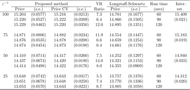
ε−1 Proposed method VR Longstaff-Schwartz Run time Inter. Price (s.e.) Price CV (s.e.) Ratio Price (s.e.) (secs) est. 100 15.204 (0.0577) 15.216 (0.0213) 7.3 14.781 (0.1677) 60 15.409 15.220 (0.0527) 15.222 (0.0209) 6.4 14.860 (0.1505) 90 (0.021) 15.229 (0.0462) 15.220 (0.0350) 12.0 14.895 (0.1351) 120 75 14.871 (0.0806) 14.882 (0.0234) 11.9 14.554 (0.1447) 60 15.183 14.876 (0.0535) 14.878 (0.0208) 6.6 14.659 (0.1254) 90 (0.019) 14.874 (0.0454) 14.873 (0.0180) 6.4 14.661 (0.1176) 120 50 14.410 (0.0714) 14.417 (0.0260) 7.5 14.252 (0.1297) 60 14.940 14.437 (0.0674) 14.420 (0.0180) 14.0 14.321 (0.1153) 90 (0.023) 14.414 (0.0498) 14.422 (0.0176) 8.0 14.355 (0.0969) 120 25 13.648 (0.0742) 13.643 (0.0317) 5.5 13.757 (0.1376) 60 14.312 13.651 (0.0678) 13.648 (0.0250) 7.4 13.770 (0.1336) 90 (0.020) 13.653 (0.0570) 13.643 (0.0221) 6.7 13.805 (0.1058) 120
Table 4.2: Comparison of standard errors (s.e.) of the option price estimate using the proposed method
without and with control variate (CV) for in-the-money option with S0 = 90. LS method price is
ob-tained using the first four Hermite polynomials as basis functions. The variance reduction (VR) ratio is calculated as the square of the ratio of standard errors in two different cases. The results are shown for different values of the run time (in seconds) for a single iteration.
To estimate the true price of the American option V0 in absence of unbiased estimators,
we aim to calculate a lower biased estimator ˆvn and an upper biased estimator Vˆn i.e. E[ˆvn]≤
V0≤E[ ˆVn]wherendenotes the number of independent replications of the respective algorithms.
Then, as explained in Glasserman [14, Pg.431], we can form a conservative confidence interval forV0as ˆvn−ln,Vˆn+Hn
wherelnandHndenote the halfwidth of a certain level of confidence
interval for lower and upper biased estimator, respectively. The estimator of the true value
V0 can then be taken as the midpoint of the confidence interval. However, due to the high
number of exercise opportunities of the American option being considered, even a reasonable implementation of the dual method proposed by Andersen and Broadie [3] is unable to provide a meaningful upper biased estimator due to the exponential increase in computational budget with the number of exercise times. Hence, to get a proxy for the true price, we useinterleaving
estimator of Longstaff and Schwartz [23]. The bias of interleaving estimator is unclear as it mixes the high bias from the backward recursion with the low bias resulting from suboptimal exercise. For our purpose, the value ofinterleaving estimator will act as a proxy to the true price and proximity to this value will provide a reasonable accuracy comparison. In our experiments,
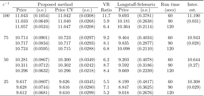
ε−1 Proposed method VR Longstaff-Schwartz Run time Inter. Price (s.e.) Price CV (s.e.) Ratio Price (s.e.) (secs) est. 100 11.043 (0.1054) 11.042 (0.0308) 11.7 9.693 (0.3781) 60 11.190 11.033 (0.0649) 11.040 (0.0268) 5.9 10.181 (0.2638) 90 (0.031) 11.057 (0.0524) 11.047 (0.0208) 6.4 10.364 (0.2114) 120 75 10.714 (0.0901) 10.723 (0.0297) 9.2 9.464 (0.4034) 60 10.943 10.717 (0.0834) 10.717 (0.0293) 8.1 9.835 (0.2877) 90 (0.028) 10.724 (0.0595) 10.715 (0.0288) 6.8 10.098 (0.2110) 120 50 10.281 (0.0867) 10.300 (0.0349) 6.2 9.203 (0.4078) 60 10.644 10.311 (0.0712) 10.302 (0.0242) 8.7 9.592 (0.3186) 90 (0.27) 10.296 (0.0632) 10.296 (0.0218) 8.4 9.669 (0.2239) 120 25 9.617 (0.0807) 9.626 (0.0345) 5.5 8.199 (0.4817) 60 10.308 9.628 (0.0744) 9.616 (0.0280) 7.1 8.847 (0.3625) 90 (0.029) 9.612 (0.0681) 9.610 (0.0299) 5.2 9.018 (0.2676) 120
Table 4.3: At-the-money option withS0= 100.
we use 4×10⁵ sample paths and the first seven Hermite polynomials and their cross products
as basis functions to calculate theinterleaving estimator (Inter. est.) in different settings where the running time of a single iteration is1.5×103 seconds.
We illustrate the performance of proposed method when compared to the LS method under the cases of in-the-money, at-the-money and out-of-the-money options in Table 4.2, 4.3 and 4.4 respectively where the reported results are based on 50 independent iterations of the algo-rithms with varying computational budgets. The computational budget for a single iteration is specified in terms of running time (in seconds) of the algorithm. In each phase of the LS algorithm, we use the same number of sample paths – 20000,30000and 40000respectively for the correspondingly increasing computational budget. We once again emphasize that in case of fast mean-reverting stochastic volatility, both the option price and optimal exercise boundary first order approximations are independent of the current level of stochastic volatility factor Yt.
Only the average of the variance σ¯2 plays a role.
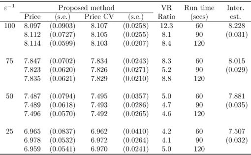
It can be observed in Table 4.2, that our proposed method performs better than the LS method for small values of the scaling parameter ε. We are also able to achieve considerable variance reduction using the control variates proposed in Section 2.2. As expected, the pric-ing accuracy reduces with increaspric-ing value of the scalpric-ing parameter ε. In Table 4.3, we can see that the proposed method provides a more accurate estimator than the lower biased LS estimator, uniformly for all values of the scaling parameterε.Further, in the case of out-of-the-money options (Table 4.4), we observed that for the given computational budget, the two phase implementation of the LS method provided insignificant estimates of the option price. This observation again emphasizes that the proposed method provides a better approach to estimate the true American option value when the stochastic volatility is fast mean-reverting.
4.2 Performance of estimator under slowly fluctuating volatility
To test the performance of the proposed estimator in the slowly fluctuating volatility setting, we consider an American put with the model parameters, initial conditions and option parameters given in Table 4.5. The numerical experiments are performed with different slow scale parameter
δ values where small values are practically relevant. The underlying sample paths are simulated with the Euler discretization scheme with time step size∆t= 10−3.We use the optimal exercise
ε−1 Proposed method VR Run time Inter. Price (s.e.) Price CV (s.e.) Ratio (secs) est. 100 8.097 (0.0903) 8.107 (0.0258) 12.3 60 8.228 8.112 (0.0727) 8.105 (0.0255) 8.1 90 (0.031) 8.114 (0.0599) 8.103 (0.0207) 8.4 120 75 7.847 (0.0702) 7.834 (0.0243) 8.3 60 8.015 7.823 (0.0620) 7.826 (0.0271) 5.2 90 (0.029) 7.835 (0.0621) 7.829 (0.0210) 8.8 120 50 7.487 (0.0794) 7.495 (0.0357) 5.0 60 7.881 7.489 (0.0618) 7.493 (0.0286) 4.7 90 (0.035) 7.496 (0.0570) 7.492 (0.0265) 4.6 120 25 6.965 (0.0837) 6.962 (0.0410) 4.2 60 7.507 6.978 (0.0532) 6.972 (0.0264) 4.1 90 (0.032) 6.959 (0.0541) 6.970 (0.0241) 5.0 120
Table 4.4: Out-of-the-money option with S0 = 110. The two phase Longstaff and Schwartz method produced very small values of option price estimator which are not reported.
boundary approximationx0+ √
δx1 derived in Section 3 to exercise the simulated sample paths.
In the case of slowly fluctuating volatility, the developed control variates do not exhibit significant variance reduction and hence, the values are not reported.
K Z0 r m2 ν2 ρ2 T
100 -1.0 0.10 -2.0 1.0 -0.3 1.0
Table 4.5: Parameters for slowly fluctuating stochastic volatility model and option parameters.
Unlike, the fast-scale stochastic volatility, the current level of volatility factorZtis extremely
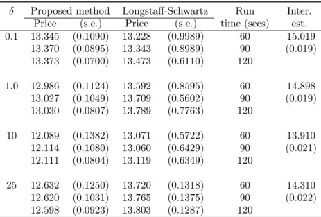
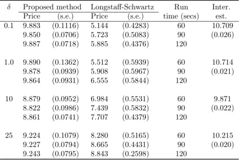
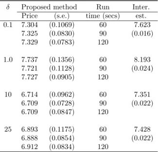
important in the slowly fluctuating stochastic volatility model. It can be observed in Table 4.6 that for δ = 0.1, our proposed method provides a slightly lower estimator than the LS method but with considerably smaller standard error. As expected, the performance of the estimator deteriorates as the value of δ increases. We implemented control variates by using approximate centered martingalesU0 and U2 but found that no considerable variance reduction is achieved in the case of slowly fluctuating volatility. This particular empirical observation motivates replacing the option maturity with the increasing arrival times of an independent Poisson process. However, the optimal exercise boundary approximation remains reasonably accurate and in Table 4.7, we can see that for a small computational budget, the proposed method provides a more accurate estimator than the lower biased LS estimator, uniformly for all values of the scaling parameter δ. Further, in the case of out-of-the-money option (Table 4.8), we observed that the two phase implementation of LS method, like in the case of fast mean-reverting stochastic volatility, provided insignificant estimates of the option price. This observation again emphasizes that the proposed method provides a better approach to estimate the true American option value in the case of both fast mean-reverting and slowly fluctuating stochastic volatility.
Remark 3. In order to compare the accuracy of the option price approximation formula in different stochastic volatility settings – fast and slow scale – we set the value of the scaling parametersε=δ = 1.We empirically observed that the boundary approximations in both the methods provide an equally accurate Monte Carlo estimator for the true American option price.
δ Proposed method Longstaff-Schwartz Run Inter. Price (s.e.) Price (s.e.) time (secs) est. 0.1 13.345 (0.1090) 13.228 (0.9989) 60 15.019 13.370 (0.0895) 13.343 (0.8989) 90 (0.019) 13.373 (0.0700) 13.473 (0.6110) 120 1.0 12.986 (0.1124) 13.592 (0.8595) 60 14.898 13.027 (0.1049) 13.709 (0.5602) 90 (0.019) 13.030 (0.0807) 13.789 (0.7763) 120 10 12.089 (0.1382) 13.071 (0.5722) 60 13.910 12.114 (0.1080) 13.060 (0.6429) 90 (0.021) 12.111 (0.0804) 13.119 (0.6349) 120 25 12.632 (0.1250) 13.720 (0.1318) 60 14.310 12.620 (0.1031) 13.765 (0.1375) 90 (0.022) 12.598 (0.0923) 13.803 (0.1287) 120
Table 4.6: Comparison of standard errors of the option price estimate using the proposed method without and with control variate (CV). The Longstaff-Schwartz method price is obtained using first four Hermite polynomials as basis functions. The results are shown for different values of the run time for single
iteration. In-the-money option withS0= 90.
Thus, when ε=δ = 1, any of the boundary approximation formula derived in Section 2 and 3 can be used to form the Monte Carlo estimator.
5
Conclusion
We introduced a new method to approximately solve the important problem of American option pricing under stochastic volatility by combining PDE asymptotic techniques with Monte Carlo simulation. We particularly study the case of an American put option with a single underlying asset. We derived closed-form approximations for the price of put option with random maturity and its optimal exercise boundary up to the first order, when volatility is driven by a fast mean-reverting or a slowly fluctuating factor. We then proposed a simulation method which uses the optimal exercise boundary approximation for price estimation and numerically showed that it performs better than a reasonable implementation of the least squares regression method under typical parameter settings and small computational budget. We also achieved significant improvement in pricing accuracy by using the derived asymptotic price approximation to form control variates in the proposed method when the stochastic volatility is fast mean-reverting. It was observed that similar improvement in pricing accuracy is not replicated when the stochastic volatility fluctuates on the slow scale. In the multiscale stochastic volatility model, it can be shown that the approximations derived separately for different scales of fluctuations essentially combine.
In our work, we randomized the maturity of the put with an exponentially distributed ran-dom variable and showed that under typical scaling parameter regimes, the exercise boundary approximations provide accurate estimators when used with Monte Carlo simulation. Under-standably, the accuracy of these approximations can be iteratively improved by replacing the fixed maturity with successively increasing arrival times of an independent Poisson process. But the number of different coefficient calculations increases with the number of boundary conditions which poses a significant computational challenge. The development of an iterative approach to achieve this task provides a promising direction for future research.
δ Proposed method Longstaff-Schwartz Run Inter. Price (s.e.) Price (s.e.) time (secs) est. 0.1 9.883 (0.1116) 5.144 (0.4283) 60 10.709 9.850 (0.0706) 5.723 (0.5083) 90 (0.026) 9.887 (0.0718) 5.885 (0.4376) 120 1.0 9.890 (0.1362) 5.512 (0.5939) 60 10.714 9.878 (0.0939) 5.908 (0.5967) 90 (0.021) 9.864 (0.0931) 6.555 (0.5844) 120 10 8.879 (0.0952) 6.984 (0.5531) 60 9.871 8.822 (0.0986) 7.439 (0.5832) 90 (0.022) 8.861 (0.0741) 7.707 (0.4379) 120 25 9.224 (0.1079) 8.280 (0.5165) 60 10.215 9.227 (0.0794) 8.665 (0.4431) 90 (0.020) 9.243 (0.0795) 8.843 (0.2598) 120
Table 4.7: At-the-money option withS0= 100.
A
Proofs
A.1 Proof of Proposition 2
It is evident from the zeroth order term P0 in (14) that we solve for the correction term P˜1 in
two separate regions. Firstly, forx > K, from (17), we get the following ODE
1 2σ¯ 2x2d2P˜1 dx2 +rx dP˜1 dx −(r+λ) ˜P1=c1x β1, where c1 =V3β12(β1−1) a01 Kβ1 + a02 xβ1 0 ! .
We use a transformation to make the linear operator L2 which has x–dependent coefficients,
into the constant coefficient heat operator. To this end, we define the new variable y = log(x). Then, the transformation to the heat equation with a source term is given by
d2P˜1 dy2 + 2r ¯ σ2 −1 dP˜1 dy − 2(r+λ) ¯ σ2 P˜1 = 2c1 ¯ σ2 exp(β1y). (25)
We use variation of parameters to solve the above ODE. The two linearly independent solutions to the homogeneous part of (25) are u1(y) = exp(β2y) and u2(y) = exp(β1y). It is easy to see
that β2 > 1 > 0 > β1. The Wronskian of the two linearly independent solutions is W(y) =
(β1−β2) exp((β1 +β2)y) = −2∆ exp(2γy) and the general solution for the ODE (25) can be
calculated as A(z)u1(y) +B(z)u2(y),where A(y) = Z − 1 W(y)F(y)u2(y)dy, B(y) = Z 1 W(y)F(y)u1(y)dy,
andF(y) = 2c1exp(β1y)/σ¯2 is the source term. The solution for the first order correction term
can then be computed via substituting back to thex variable
˜ P1(x) =a1xβ1 + ˜a1xβ2− V3β12(β1−1) ¯ σ2∆ log(x) a01 x K β1 +a02 x x0 β1 , forx > K,
δ Proposed method Run Inter. Price (s.e.) time (secs) est. 0.1 7.304 (0.1069) 60 7.623 7.325 (0.0830) 90 (0.016) 7.329 (0.0783) 120 1.0 7.737 (0.1356) 60 8.193 7.721 (0.1128) 90 (0.024) 7.727 (0.0905) 120 10 6.714 (0.0962) 60 7.351 6.709 (0.0728) 90 (0.022) 6.709 (0.0847) 120 25 6.893 (0.1175) 60 7.428 6.888 (0.0854) 90 (0.022) 6.912 (0.0834) 120
Table 4.8: Out-of-the-money option with S0 = 110. The two phase Longstaff and Schwartz method produced very small values of option price estimator which are not reported.
for unknown constants a1 anda˜1.
Similarly, in the region x0 < x≤K, from the solution in (14), we get
1 2σ¯ 2x2d2P˜1 dx2 +rx dP˜1 dx −(r+λ) ˜P1 =c2x β1 +c 3xβ2, where c2 =V3β12(β1−1) a02 xβ1 0 , c3 =V3β22(β2−1) b01 Kβ2.
The solution in this case is
˜ P1(x) =a2xβ1+a3xβ2+ V3log(x) ¯ σ2∆ b01β22(β2−1) x K β2 −a02β12(β1−1) x x0 β1 , for x0< x≤K,
for unknown constants a2 anda3.Forx≤x0, we haveP˜1(x) = 0.
To solve for the unknown constants, we first note that as β2 >0, it is easy to see from the
condition lim
x↑∞
˜
P1(x) = 0that˜a1= 0.For the remaining constantsa1, a2, a3, we use the continuity
condition at x=K and x=x0, and differentiability condition at x=K to obtain three linear
equations. After a fair bit of algebra we can solve for the constants. Then,P˜1(x) is given by the
formula stated in Proposition 2.
For the correction term in the expansion of the optimal exercise boundary, we refer to (11) and get ˜ x1=− ∂P˜1 ∂x x0 .∂2P0 ∂x2 x0
A.2 Proof of Lemma 1
In this proof, we do not explicitly mention the dependence of x0(·) on z for ease of notation.
For smooth functionP0, we compute the following by differentiating (22) with respect toz
1 2f 2(z)x2∂2V ∂x2 +rx ∂V ∂x −(r+λ)V+f(z)f 0(z)x2∂2P0 ∂x2 = 0,
wheref0(z) =∂f(z)/∂z.In order to solve the above equation, we first consider the homogeneous equation L2V = 0.We use a transformation to make the linear operator L2 which has (x, z)– dependent coefficients, into the z–dependent coefficient heat operator as shown below. To this end, we define the new variable y= log(x). Then, the transformation to the heat equation is
1 2f 2(z)∂2V ∂y2 + r−1 2f 2(z)∂V ∂y −(r+λ)V = 0.
In case ofx > K, the source term is given byc1xβ1 where
c1 =−f(z)f0(z)β1(β1−1) a01/Kβ1 +a02/xβ01
.
We use variation of parameters technique to conclude thatV is given by
V(x, z) =a1 x x0 β1 +f 0(z)β 1(β1−1) f(z)∆ logx a01 x K β1 +a02 x x0 β1 , for x > K.
Similarly, in the regionx0< x≤K, we get
1 2f 2(z)d2V dy2 + r−1 2f 2(z)dV dy −(r+λ)V =c2x β1 +c 3xβ2, where c2 =−f(z)f0(z)β1(β1−1) a02 xβ1 0 , c3 =−f(z)f0(z)β2(β2−1) b01 Kβ2.
The solution in this case is
V(x, z) =a2 x x0 β1 +a3 x K β2 − f 0(z) log(x) f(z)∆ b01β2(β2−1) x K β2 −a02β1(β1−1) x x0 β1 , for x0< x≤K.
From the expression ofV,we can see that for fixedz, it remains continuously differentiable with respect tox in the respective regions. Thus, we expect that the function and its first derivative also remain continuous across the boundary. Hence, we can find the unknown coefficientsa1, a2
and a3 by using the continuity condition at x = x0 and differentiability condition at x = K.
This procedure provides us the following:
a1 =− f0(z) 2f(z)∆2 a01β1(β1−1) +b01β2(β2−1) x0 K β2− x0 K β1 − f 0(z) f(z)∆ β1(β1−1) a01( x0 K) β1log(K) +a 02log(x0) −b01β2(β2−1) x0 K β2 log(x0 K) , (26) a2 =− f0(z) 2f(z)∆2 x0 K β2 a01β1(β1−1) +b01β2(β2−1)(1 + 2∆ log(K)) − f 0(z) f(z)∆log(x0) a02β1(β1−1)−b01β2(β2−1) x0 K β2 , (27) a3 = f0(z) 2f(z)∆2 a01β1(β1−1) +b01β2(β2−1)(1 + 2∆ log(K)) . (28)
A.3 Proof of Proposition 3
For the regionx > K, plugging back V in (23), we get the following PDE
L2P1 =c4xβ1+c5xβ1(1 +β1log(x)) with c4=− √ 2ρ2ν2β1a1f(z)/xβ01, c5 =− √ 2ρ2ν2 ∆ β1(β1−1)f 0(z) a 01/Kβ1+a02/xβ01 .
By defining a new variable y = log(x), we can reduce the above equation to a heat equation with only z–dependent coefficients and a source term. The transformation is given by,
1 2f 2(z)∂2P1 ∂y2 + r−1 2f 2(z)∂P1
∂y −(r+λ)P1 =c4exp(β1y) +c5(1 +β1y) exp(β1y).
In the remaining proof, we do not explicitly mention the dependence of x0(·) on z for ease of
notation.The solution using variation of parameters technique is given by
P1(x, z) = ˜η1xβ1 − c4 ∆f2(z)x β1log(x)− c5 2∆2f2(z)x β1log(x)(β 2+β1∆ log(x)), for x > K,
whereη˜1 is an unknown coefficient dependent on z. For x0 < x ≤K, plugging back V in (23),
we get the following PDE
L2P1 =c6xβ1+c7xβ2 −c8xβ2(1 +β2log(x)) +c9xβ1(1 +β1log(x)) with c6 =− √ 2ρ2ν2f(z)a2β1/xβ01, c7=− √ 2ρ2ν2f(z)a3β2/Kβ2 c8= −√2ρ2ν2f0(z)β2(β2−1) ∆ b01 Kβ2 c9 = −√2ρ2ν2f0(z)β1(β1−1) ∆ a02 xβ1 0 .
We repeat the procedure discussed above to get, forx0 < x≤K,
P1(x, z) = ˜η2xβ1+ ˜η3xβ2 − c6 ∆f2(z)x β1log(x) + c7 ∆f2(z)x β2log(x) + c8 2∆2f2(z)x β2log(x)(β 1−∆β2log(x))− c9 2∆2f2(z)x β1log(x)(β 2+ ∆β1log(x)),
whereη˜2 and η˜3 are unknown coefficients dependent on z. Let us define V2(z) := √ 2ρ2ν2 ∆f2(z).Then, we have P1(x, z) =η1 x x0 β1 +V2(z)a1f(z)β1log(x) x x0 β1 +V2(z)f 0(z) 2∆2 β1(β1−1) log(x) β2 +β1∆ log(x) a01 x K β1 +a02 x x0 β1 , for x > K, P1(x, z) =η2 x x0 β1 +η3 x K β2 +V2(z)a2f(z)β1log(x) x x0 β1 −V2(z)a3f(z)β2log(x) x K β2 −V2(z)f 0(z) 2∆2 β2(β2−1)b01log(x) β1−β2∆ log(x) x K β2 +V2(z)f 0(z) 2∆2 β1(β1−1)a02log(x) β2+β1∆ log(x) x x0 β1 , for x0 ≤x≤K,
for unknown coefficients η1, η2 and η3. Next, we use the continuity condition at x = x0 and
x=K and differentiability condition atx=K to calculate these coefficients which are given as follows η1 =V2(z) h a01β1β2(β1−1)f0(z) 1− K x0 β1−β2− 2a01∆2β1(β1−1)f0(z) log(K) 2 +β1log(K) −2a01∆β12(β1−1)f0(z) log(K) K x0 β1−β2 −2a02∆β1(β1−1)f0(z) log(x0) K x0 β1 β2+ ∆β1log(x0) −b01β1β2(β2−1)f0(z) K x0 β1−β2 −1 + 2b01∆β22(β2−1)f0(z) log(K) K x0 β1−β2 −1 −2b01∆β1β2(β2−1)f0(z) K x0 β1−β2 log(K)−log(x0) + 2b01∆2β22(β2−1)f0(z) K x0 β1−β2 log2(K)−log2(x0) −2(a1−a2)∆2β1β2f(z) log(K) K x0 β1− 2(a1−a2)∆2β1f(z) K x0 β1 K x0 β1−β2 − β1log(K) + 2a2∆2β1f(z) K x0 β1 β1log(x0)−1 −2(a2β2log(x0)−a1)∆2β1f(z) K x0 β1 −2a3∆2β2f(z) K x0 β1−β2 − 1 −4a3∆3β2f(z) K x0 β1−β2 log(K)−log(x0) i 4∆3(K/x0)β1 , (29) η2 =−V2(z) h a01β1β2(β1−1)f0(z) x0 K β2 + 2a01∆β21(β1−1)f0(z) log(K) x0 K β2 −4a02∆2β1β2f0(z) log(x0) + 2a02∆2β12(β1−1)f0(z) log2(x0) +b01β1β2(β2−1)f0(z) x0 K β2− 2b01∆β22(β2−1)f0(z) log(K) x0 K β2 + 2b01∆β1β2(β2−1)f0(z) x0 K β2 log(K)−log(x0) −2b01∆2β22(β2−1)f0(z) x0 K β2 log2(K)−log2(x0) + 2(a1−a2)∆2β1f(z) K x0 β1−β2 + 4a2∆2β1f(z) log(x0) + 2a3∆2β2f(z) x0 K β2 + 2a3∆3β2f(z) x0 K β2 log(K)−log(x0) i 4∆3, (30) η3 =V2(z) h a01β1(β1−1)f0(z) β2+ 2∆β1log(K) +b01β2(β2−1)f0(z) β1−2∆2log(K) 2 +β2log(K) + 2a3∆2β2f(z) 1 + 2∆ log(K) + 2(a1−a2)∆2β1f(z) K x0 β1i 4∆3. (31)
B
Implementation of control variates
In order to achieve variance reduction for the proposed Monte Carlo price estimator, we use control variates as introduced in Sections 2.2 and 3.2. Here, we discuss their implementation in the numerical examples.
B.1 Fast Factor Control Variate
Let us recall the centered martingale which is used as a control variate under the fast mean-reverting stochastic volatility. It is given by
ˆ U0(P(1);xb) = Z τˆ 0 e−rs ∂ ∂x(P0+ √ εP1)(Xs)f(Ys)XsdWs(1),
whereτˆis the exercise time approximated using the boundary approximationx0+ √
εx1.
In the simulation method, we discretize the time scale with a time step ∆t= 10−3. Thus, the total number of time steps required to sample a path of the underlying processXfor pricing an American put with maturity T is L = T /∆t. Next, we generate a set of N independent underlying sample paths for X and Y using the Euler discretization scheme and denote them as X0(i), X1(i),· · · , XL(i)Ni=1 and Y0(i), Y1(i),· · ·, YL(i)Ni=1 where to simplify the notation we have used Xn(i) := Xn(i∆)t and Yn(i) := Yn(∆i)t for n = 0,1,· · ·, L. On these sample paths, we use the
exercise policy based on the approximate optimal exercise time defined as
ˆ
τ := min
n≥0 :Xn≤x0+ √
εx1 ∧L.
The control variate C(i) which approximates Uˆ0(P(1);x
b) for the ith underlying path is formed
as follows by using the explicit formulas for the derivatives of P0 andP1
C(i):= ˆ τ(i)−1 X n=0 e−r(n+1)∆t h DP0(Xn(i)) + √ εDP1(Xn(i)) i f(Yn(i))Xn(i) √ ∆tNi,n(1)+1, where DP0(Xn) := a01βK1 XKnβ1 −1 +a02βx10 Xx0nβ1 −1 if Xn> K, b01βK2 XKnβ2 −1 +a02βx10 Xx0nβ1 −1 −1 if x0 < Xn≤K, −1 if Xn≤x0, √ εDP1(Xn) := ˆ a1βx10 Xn x0 β1−1 − V3β12(β1−1) ¯ σ2∆K a01 Xn K β1−1 +a02 Xn x0 β1−1 (1 +β1log(Xn)) if Xn> K, ˆ a3βx10 Xn x0 β1−1 + ˆa4βx20 Xn K β2−1 + V3 ¯ σ2∆ b 01β22(β2−1) K Xn K β2−1 (1 +β2log(Xn)) −a02β21(β1−1) x0 Xn x0 β1−1 (1 +β1log(Xn)) if x0< Xn≤K, 0 if Xn≤x0, and Ni,(1)1,· · · , Ni,(1)τˆ(i)
is the realization of a sequence of independent standard normal random variables generated to simulate the ith sample path of Brownian motion W(1) in the Euler scheme.
B.2 Slow Factor Control Variate
In the case of slowly fluctuating volatility, the first martingale is
ˆ U0(P(1);xb) = Z τˆ 0 e−rs ∂ ∂x(P0+ √ δP1)(Xs, Zs)f(Zs)XsdWs(1).
Here, the derivative ofP0 andP1 with respect toxcan be calculated explicitly from the results
in Section 3. The other centered martingale is
ˆ U2(P(1);xb) = Z τˆ 0 e−rs ∂ ∂z(P0+ √ δP1)(Xs, Zs)h(Zs)dWs(3). (32)
In (32), the derivative ∂P0/∂z is denoted asV which is given explicitly in Lemma 1. The main
difficulty is to calculate the derivative ofP1with respect tozas it has an implicit dependence on
the variable. To overcome this issue, we use a finite difference estimate of∂P1/∂z. We suppress
the dependence of x0(·) on zfor notational convenience.
Thus, the control variate C(i) which approximates Uˆ0(P(1);xb) + √ δUˆ2(P(1);xb) for the ith underlying path isC(i) :=C(i) 1 + √ δC2(i), where C1(i):= ˆ τ(i)−1 X n=0 e−r(n+1)hDP0(Xn(i), Zn(i)) + √ δDP1(Xn(i), Zn(i)) i f(Zn(i))Xn(i)√∆tNi,n(1)+1, DP0(Xn, Zn) := a01βK1 XKn β1−1 +a02βx10 Xx0n β1−1 if Xn> K, b01βK2 XKnβ2 −1 +a02βx10 Xx0nβ1 −1 −1 if x0< Xn≤K, −1 if Xn≤x0, DP1(Xn, Zn) := η1β1 Xn Xn x0 β1 + V2(Zn)a1β1f(Zn) Xn Xn x0 β1 (1 +β1log(Xn)) +V2(Zn)β1(β1−1)f0(Zn) 2∆2X n a01 XKn β1 +a02 Xx0n β1
× β2(1 +β1log(Xn)) + ∆β1log(Xn)(2 +β1log(Xn)) if Xn> K, η2β1 Xn Xn x0 β1 + η3β2 Xn Xn K β2 +V2(Zn)a2β1f(Zn) Xn Xn x0 β1 1 +β1log(Xn) −V2(Zn)a3β2f(Zn) Xn Xn K β2 1 +β2log(Xn) −V2(Zn)b01β2(β2−1)f0(Zn) 2∆2X n Xn K β2 × β1−∆β2log(Xn) 1 +β2log(Xn) −∆β2log(Xn) +V2(Zn)a02β1(β1−1)f0(Zn) 2∆2Xn Xn x0 β1 × β2+ ∆β1log(Xn) 1 +β1log(Xn) + ∆β1log(Xn) if x0 < Xn≤K, 0 if Xn≤x0. Further, C2(i):= ˆ τ(i)−1 X n=0 e−r(n+1)∆thV(Xn(i), Zn(i))+√∆P1z(Xn(i), Zn(i))i√2ν2 √ ∆tρ2Ni,n(1)+1+ q 1−ρ2 2N (3) i,n+1 ,
and for smallh >0,
P1z(Xn, Zn) := −P1(Xn, Zn+ 2h) + 4P1(Xn, Zn+h)−3P1(Xn, Zn) h . Ni,(1)1,· · ·, Ni,(1)ˆτ(i) and Ni,(3)1,· · ·, Ni,(3)ˆτ(i)
are the realizations of sequence of independent stan-dard normal random variables generated to simulate the ith sample path of Brownian motion
References
[1] A. Agarwal and S. Juneja. Nearest neighbor based estimation technique for pricing Bermu-dan options. International Game Theory Review, 17(01):1540002, 2015.
[2] L. Andersen. A simple approach to the pricing of Bermudan swaptions in the multi-factor Libor market model. Available at SSRN 155208, 1999.
[3] L. Andersen and M. Broadie. Primal-dual simulation algorithm for pricing multidimensional American options. Management Science, 50(9):1222–1234, 2004.
[4] D. Belomestny. Pricing Bermudan options by nonparametric regression: Optimal rates of convergence for lower estimates. Finance and Stochastics, 15(4):655–683, 2011.
[5] B. Bouchard, N. El Karoui, and N. Touzi. Maturity randomization for stochastic control problems. The Annals of Applied Probability, 15(4):2575–2605, 2005.
[6] M. J. Brennan and E. S. Schwartz. The valuation of American put options. The Journal of Finance, 32(2):449–462, 1977.
[7] M. Broadie and P. Glasserman. Pricing American-style securities using simulation. Journal of Economic Dynamics and Control, 21(8):1323–1352, 1997.
[8] M. Broadie and P. Glasserman. A stochastic mesh method for pricing high-dimensional American options. Working paper, 1998.
[9] P. Carr. Randomization and the American put. Review of Financial Studies, 11(3):597–626, 1998.
[10] J. C. Cox, S. A. Ross, and M. Rubinstein. Option pricing: A simplified approach. Journal of Financial Economics, 7(3):229–263, 1979.
[11] J. Duistermaat, A. E. Kyprianou, and K. van Schaik. Finite expiry Russian options. Stochas-tic processes and their applications, 115(4):609–638, 2005.
[12] J.-P. Fouque and C.-H. Han. A martingale control variate method for option pricing with stochastic volatility. ESAIM: Probability and Statistics, 11(1):40–54, 2007.
[13] J.-P. Fouque, G. Papanicolaou, R. Sircar, and K. Sølna. Multiscale stochastic volatility for equity, interest rate, and credit derivatives. Cambridge University Press, Cambridge, 2011. [14] P. Glasserman. Monte Carlo methods in financial engineering, volume 53. Springer, 2004. [15] R. B. Gramacy and M. Ludkovski. Sequential design for optimal stopping problems.
Tech-nical report, University of California at Santa Barbara, 2014.
[16] S. Heston. A closed-form solution for options with stochastic volatility with applications to bond and currency options. Review of Financial Studies, 6(2):327–343, 1993.
[17] J. Hull and A. White. The pricing of options on assets with stochastic volatilities. The Journal of Finance, 42(2):281–300, 1987.
[18] S. Ikonen and J. Toivanen. Componentwise splitting methods for pricing American options under stochastic volatility. International Journal of Theoretical and Applied Finance, 10 (02):331–361, 2007.
[19] S. Ikonen and J. Toivanen. Efficient numerical methods for pricing American options under stochastic volatility. Numerical Methods for Partial Differential Equations, 24(1):104–126, 2008.
[20] F. Kleinert and K. Van Schaik. A variation of the Canadisation algorithm for the pricing of American options driven by Lévy processes. arXiv preprint arXiv:1304.4534, 2013. [21] A. E. Kyprianou and M. R. Pistorius. Perpetual options and Canadization through
fluctu-ation theory. The Annals of Applied Probability, 13(3):1077–1098, 2003.
[22] T. Leung, K. Yamazaki, and H. Zhang. An analytic recursive method for optimal multiple stopping: Canadization and phase-type fitting. Technical report, Columbia University, 2014.
[23] F. A. Longstaff and E. S. Schwartz. Valuing American options by simulation: A simple least-squares approach. Review of Financial studies, 14(1):113–147, 2001.
[24] B. R. Rambharat and A. E. Brockwell. Sequential Monte Carlo pricing of American-style options under stochastic volatility models. The Annals of Applied Statistics, 4(1):222–265, 2010.
[25] M. Rubinstein. Nonparametric tests of alternative option pricing models. The Journal of Finance, 40(2):455–480, 1985.
[26] M. Schroder. Changes of numeraire for pricing futures, forwards, and options. Review of Financial Studies, 12(5):1143–1163, 1999.
[27] S. H. M. Ting, C.-O. Ewald, and W.-K. Wang. On the investment–uncertainty relationship in a real option model with stochastic volatility. Mathematical Social Sciences, 2013. [28] N. Touzi. American options exercise boundary when the volatility changes randomly.