Quantum Effects and Dynamics in
Hydrogen-Bonded Systems: A First-Principles
Approach to Spectroscopic Experiments
Dissertation zur Erlangung des Grades
“Doktor der Naturwissenschaften”
am Fachbereich Physik
der Johannes Gutenberg-Universit¨
at
in Mainz
Jochen Schmidt
geboren in Mainz
Contents
1 Introduction 1
2 Basic Theory 5
2.1 Density Functional Theory . . . 5
2.1.1 Motivation . . . 5
2.1.2 The Born-Oppenheimer Approximation . . . 7
2.1.3 The Hohenberg-Kohn Theorem . . . 9
2.1.4 The Kohn-Sham Method . . . 14
2.1.5 The Local-Density Approximation . . . 18
2.1.6 Gradient Corrected functionals . . . 19
2.2 Pseudopotentials and Basis Sets . . . 21
2.2.1 The Pseudopotential Approximation . . . 21
2.2.2 Basis sets . . . 23
2.3 Computational Realizations . . . 27
2.3.1 Gaussian and Plane Waves Method (GPW) . . . 27
2.3.2 Gaussian and Augmented Plane Waves Method (GAPW) . 30 2.4 Molecular Dynamics Simulations . . . 34
2.4.1 Overview . . . 34
2.4.2 Born-Oppenheimer MD . . . 35
2.4.3 Car-Parrinello MD . . . 36
2.4.4 Realization of the NVT-Ensemble . . . 38
3 Calculation of Spectroscopic Properties 41 3.1 Introduction . . . 41
3.2 Ground State Properties . . . 43
3.2.1 Nuclear Quadrupole Coupling Constants (NQCC) . . . 43
3.2.2 Calculation of Electric Field Gradients . . . 47
ii Contents
3.2.3 Relaxation via Quadrupole Couplings . . . 49
3.3 Second-Order Properties . . . 53
3.3.1 General . . . 53
3.3.2 Chemical Shifts . . . 54
3.3.3 The gauge origin problem . . . 56
4 The Path Integral Formalism 59 4.1 Motivation . . . 59
4.2 Formal Derivation of Path Integrals . . . 61
4.3 Path Integrals in MD Simulations . . . 64
4.3.1 Representation with Ring Polymers . . . 64
4.3.2 The Staging Transformation . . . 65
4.3.3 Finite-Discretization Errors . . . 67
5 Nuclear Quantum Effects in Molecular Systems 69 5.1 Motivation . . . 69
5.2 Staging Transformation and Spectroscopic Properties . . . 71
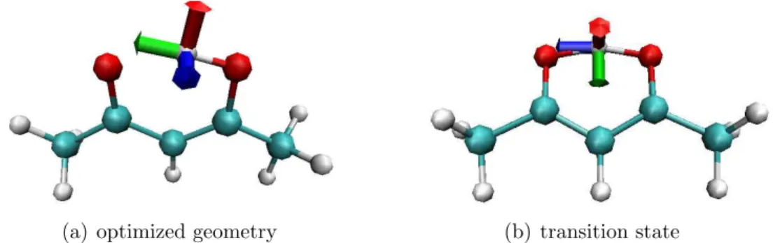
5.3 Tunneling Effects in Acetylacetone . . . 77
5.3.1 Introduction . . . 77
5.3.2 Proton Density from a Path Integral Simulation . . . 78
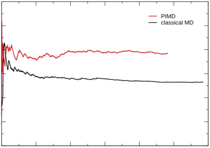
5.3.3 Electric Field Gradients: Classic vs. Quantum MD . . . . 83
5.3.4 NMR: Classical vs. Quantum MD . . . 86
5.4 Nuclear quadrupole couplings in benzoic acid . . . 91
5.4.1 Introduction . . . 91
5.4.2 Quantum effects on the NQCC . . . 93
5.5 Conclusions . . . 96
6 Quadrupole Relaxation in Water 99 6.1 Introduction . . . 99
6.2 EFG in GAPW - Tests and Benchmarks . . . 100
6.3 MD Simulation of Liquid Water . . . 103
6.4 Autocorrelation and Relaxation . . . 107
Contents iii
7 Constant Pressure Simulations 119
7.1 Theoretical Background . . . 119
7.1.1 Motivation . . . 119
7.1.2 Basic Thermodynamics . . . 120
7.1.3 Stress-Tensor . . . 122
7.1.4 Pressure and Periodic Boundary Conditions . . . 127
7.2 Stress Tensor in the GPW framework . . . 128
7.2.1 Forces in GPW . . . 128
7.2.2 Grid Independent Terms of the Stress Tensor . . . 132
7.2.3 Grid Dependent Terms of the Stress Tensor . . . 133
7.2.4 Test of the Implementation . . . 138
7.3 Simulation of Liquid Water at Ambient Conditions . . . 139
7.3.1 Prelude: TheN P T Integrator . . . 139
7.3.2 Introduction . . . 141
7.3.3 Technical Details . . . 142
7.3.4 Results . . . 144
7.4 Conclusions . . . 155
8 Summary and Outlook 157
A Derivation of the Stress Tensor 161
B Technical Details: Simulations 164
C Technical Details: NMR Measurements 165
D Atomic units 167
E Abbreviations 169
1
Introduction
The year 1985 can be considered a milestone for the field of computational mate-rials science. Car and Parrinello published their “Unified Approach for Molecular Dynamics and Density-Functional Theory” [1]. This work provided a novel basis for molecular dynamics simulations based on a potential energy surface computed from electronic structure, nowadays known as “Car-Parrinello molecular dynam-ics”. Secondly, Cray Research released the Cray-2 supercomputer, yielding a performance of 3.9 GigaFLOPS1, which was not outperformed by another
ma-chine until 1990. Starting in the late 80’s, the power of the new techniques, both conceptual and technical, led to an explosion of the activity in this field. 22 years later, the fastest supercomputer is BlueGene/L with 280 TeraFLOPS. Interest-ingly, both Cray-2 and BlueGene/L have been built for the Lawrence Livermore National Laboratory, where also a part of this work has been conducted.
While the Cray-2 cannot be found on 2007’s TOP500 list of the fastest super-computers2, the Car-Parrinello method is still in widespread use. By July 2007,
the original paper has been cited in more than 4000 publications. The first appli-cations of ab-initio molecular dynamics were limited to a few atoms and several tens of femtoseconds, both using the Car-Parrinello method and other approaches, such as Born-Oppenheimer molecular dynamics. Modern computer clusters, such as BlueGene/L, which provides the impressive number of 131,000 processors, en-able the ab-initio treatment of thousands of atoms and simulation times up to several nanoseconds. This has been achieved by pure computational power on the one hand, but also by developing efficient and sophisticated algorithms. “Linear scaling techniques” that circumvent the cubic scaling with the system size ex-hibited by many conventional schemes, are mentioned here as an example that
1Floating Point Operations Per Second 2seehttp://www.top500.org/
2 1 Introduction
opens the way for the modeling of biological systems. Before, these have been ac-cessible only with the help of methods that use empirical and pre-parameterized potentials.
Typically, a molecular dynamics simulation is carried out for investigating the energetics and structure of a system under conditions that include physical pa-rameters such as temperature and pressure. Ab initio quantum chemical methods, which form the basis of the dynamics scheme, have also proven to be capable of predicting other experimentally accessible quantities, e.g. spectroscopic param-eters. Still, the combination of these two features, dynamics simulations and property calculations, is not commonly used, although it provides valuable infor-mation, for instance the temperature dependence of the parameters. This is due to the fact that both types of calculations are computationally very demanding, leading to an immense effort for the combined scheme.
Furthermore, conventional molecular dynamics consider the nuclei as classical particles that are subject to the forces created by the potential due to the quantum mechanically treated electrons. Not only motional effects, but also the quantum nature of the nuclei are expected to influence the properties of a molecular system. This has already been investigated using approximate methods, but a scheme based on path integrals provides a computational method for the rigorous inclusion of such effects at a high level of accuracy.
In this work, the computational methods mentioned above have been combined, aiming for a more realistic and complete description of properties that are accessi-ble via NMR3experiments, such as the NMR chemical shift or Nuclear Quadrupole
Coupling Constants. Isotope effects, caused by the quantum mechanical behavior of the involved particles, are well known and experimentally observed in NMR. Here, a computational approach for handling them, based on ab-initio path in-tegral methods is presented, allowing a direct comparison to the respective ex-periments. With the help of efficiently parallelized computer codes, a consistent description on the first-principles level of theory could be achieved, leading to quantitative agreement with the experiment.
Besides the disregard of nuclear quantum effects, pseudopotentials are commonly
1 Introduction 3
used. These treat the core electrons of an atom as a contribution to an effective potential, leading to computational savings because only the valence electrons have to be taken into account explicitly in the actual simulation. Especially in the solid state, where periodic boundary conditions are applied, this method is crucial. Unfortunately, for the calculation of spectroscopic properties, this approach is not sufficient. This holds in particular for spectroscopic parameters which are sensitive to the interaction of nuclei with the core electrons. Therefore, in the second part of this work, a new method for all-electron calculations in periodic systems has been used for the evaluation of quadrupole interactions that lead to relaxation in water, both for 17O and 2H. Again, this scheme has been combined
with molecular dynamics simulations, allowing for a realistic description of the dynamics and therefore the relaxation mechanisms.
In the last part of this work, a technical contribution to the development of the quantum chemical program package CP2K4 has been made. This code employs a newly developed method that combines the advantages of different basis sets, lead-ing to a speed-up of the calculations and also allowlead-ing for sophisticated schemes as the above mentioned all-electron calculations. Such calculations are supposed to resemble the experiment, which in many cases is carried out under ambient conditions, i.e. temperature and pressure are defined by the environment. There-fore, the calculation of the internal pressure of a computed system is necessary, which has been implemented in this work. Subsequently, water under ambient conditions has been simulated using the new routines.
2
Basic Theory
2.1 Density Functional Theory
2.1.1 Motivation
The ab-initio description of molecular systems in a quantum mechanical frame-work commonly starts with the Schr¨odinger equation. Theories that include spin and relativistic effects are available, e.g. Pauli or Dirac equation, but they are used rarely because for most compounds the Schr¨odinger equation is sufficient. For a system consisting ofn electrons and N nuclei, it is given by:
Hχ(r1, . . . ,rn,R1, . . .RN) = Eχ(r1, . . . ,rn,R1, . . .RN). (2.1)
The Hamiltonian H is defined as
H = X i − ~ 2 2me ∇2i +X I − ~ 2 2MI ∇2I+1 2 X i6=j e2 |ri −rj| + 1 2 X I6=J e2Q IQJ |RI −RJ| −X iI e2Q I |ri−RI| . (2.2)
Electrons are denoted by small indices (i), nuclei by capital ones (I), r and R are the position operators of the electrons and nuclei, respectively1. M is the
nuclear mass, me the mass of the electron, Q and e are the charges of the nuclei and electrons. Here, gaussian units are used, but in lateron, atomic units will be introduced.
The Schr¨odinger equation suggests, that the exact wave function is the most straightforward quantity to use in quantum chemical calculations. But actually, it turns out to be difficult to handle and inconvenient for a practical computation.
1Throughout this work vectors are printed in bold letters.
6 2 Basic Theory
Let a model system consist of 10 particles. It is described by a wave function of the form
χ(r1,r2, . . . ,r10). (2.3)
During a numerical calculation, this wave function has to be stored on a spatial grid. If each axis is represented by only 10 points and each value of χis given by a 10 bytes variable, the needed total data capacity is:
10 bytes point × 10 points axis 3axes×10particles = 1031bytes. (2.4)
That means, that the storage of this wave function on DVDs, each being capable of 10 GB, requires 1021 DVDs. One DVD weighs about 10 grams, resulting in a total weight of 1016 tons. If these disks were shipped with trucks with a length of 10 m, each carrying 10 tons, they would line up to 1013 km, corresponding to
100,000 times the distance between sun and earth.
Although the capacity of modern storage media is increasing rapidly, such an amount of data will cause severe problems. Thus, approximations are needed to reduce the data, that are actually needed during the calculation. Most of these methods are based on the fact, that anti-symmetric many-particle wave functions can be written as a linear combination of Slater determinats of atomic basis functions. So, the first approach is to express the wave function as single
Slater determinant of the occupied atomic states, which is referred to as Hartree-Fock wave function. Starting from this, several improvements are possible. A natural extension is the usage of additional, unoccupied states or the description of the wave function by a sum of determinants. In principle, that is the idea of the Confuguration-Interaction- or the Coupled-Cluster Method. These can treat molecular systems with a high accuracy. The Møller-Plesset Theory, on the other hand, includes many-particle effects as quantum mechanical perturbations. A detailed introduction to these techniques can be found in Ref. [2].
The above-mentioned methods are referred to as Post-Hartree-Fock methods. They can yield highly accurate results, but require an enormous computational effort. Therefore, they are limited to relatively small systems. The Density Func-tional Theory (DFT) follows a different approach where only the probability
den-2.1 Density Functional Theory 7 sity ρ(r) = n Z · · · Z |χ(r,r2, . . . ,rn)|2 dr2· · ·drn (2.5)
instead of the whole wave function is used. The density is a function of only one
position variable, but according to theHohenberg-Kohn Theorem it contains the same information as the wave function. Or, putting it the other way around, the wave function, that depends on 3n variables, plusn spin variables, contains more information than is actually needed, because the Hamiltonian of Eq. (2.2) consists of only one- and two-electron spatial terms.
2.1.2 The Born-Oppenheimer Approximation
The Schr¨odinger equation contains nuclear and electronic degrees of freedom and both are treated under equal footing. Thus, the wave function of the systems also depends on the positions of the electrons and nuclei. While both types of particles appear to be similar in theory, there is a significant difference: The masses are separated by several orders of magnitude. For instance, the proton mass is approximately 2000 times larger than the mass of an electron. This fact allows for a further simplification of the problem, often referred to as the Born-Oppenheimer approximation [3].
In the first step, a new parameter is introduced, which only depends on the masses of the involved particles:
κ= me
M . (2.6)
In this equation M can be one of the ionic masses MI. For simplification, it will be assumed in the following, that MI = M for all I. Using the new parameter κ, the Hamiltonian of Eq. (7.1) can be rewritten. Therefore, some abbreviations have to be defined: H = X i − ~ 2 2me ∇2 i + X I − ~ 2 2MI ∇2 I+ 1 2 X i6=j e2 |ri −rj| + 1 2 X I6=J e2Q IQJ |RI −RJ| −X iI e2Q I |ri−RI| = TE +TN +U = H0+TN . (2.7)
8 2 Basic Theory
Using these equations, the kinetic energy of the ions TN is
TN =κH1, H1 = X I − ~ 2 2me ∇2 I . (2.8)
The Hamiltonian H thus reads
H=H0+κH1 . (2.9)
Since κ 1, the ionic kinetic energy can be treated as perturbation. From this approximation, it can be found that the evolution of the nuclei is decoupled from the electronic degrees of freedom. Thus, the total wave function can be written as a product of an electronic and a nuclear wave function:
χ(r1, . . . ,rn,R1, . . . ,RN) = ΨR1,...,RN(r1, . . . ,rn) ξ(R1, . . . ,RN) . (2.10)
This is referred to as the Born-Oppenheimer approximation. The positions of the nuclei {R1, . . .RN} are only parameters in the electronic wave function. Further-more, the nuclei will be treated as classical point-particles. This is done in the framework of the WKB2 method, which will not be explained in detail here. An
introduction to that can be found in [4]. The dynamics of the nuclei can thus be described by a Newtonian equation of motion, i.e.
MIR¨I =−∇I
Z
dr Ψ∗H0Ψ. (2.11)
In conclusion, it can be stated, that the nuclei are moving as classical particles in an effective potential, that is created by the electrons. The electrons are the only particles that are treated quantum mechanically here, but later on, there are special cases where the nuclei have to be included in the quantum mechanical framework via the path integral method (see Chapter 4). Employing this approxi-mation, which is justified in many cases, only the following Schr¨odinger equation for the electrons has to be solved:
HelΨ
R1,...,RN(r1, . . . ,rn) =ER1,...,RNΨR1,...,RN(r1, . . . ,rn), (2.12)
2.1 Density Functional Theory 9 where Hel = X i − ~ 2 2me∇ 2 i + 1 2 X i6=j e2 |ri−rj| −X iI e2Q I |ri−RI| = X i − ~ 2 2me ∇2 i + 1 2 X i6=j e2 |ri−rj| +X i vext(ri) . (2.13)
In Eq. 2.13 the interaction between electrons and nuclei has been replaced by a generalized potential vext. Both the electronic wave function and the eigenvalues depend parametrically on the positions of the nuclei RI. In contrast to the total wave function from Eq. 2.1, χ, the number of degrees of freedom is 3n instead of 3N+ 3n, which is a major improvement of the Born-Oppenheimer approxima-tion compared to the exact problem. Eq. 2.13 is a time-independent Schr¨odinger equation for the electrons within the constant field of the nuclei. The dynamics of the latter is now described in the framework of classical Newtonian mechanics.
While the previous equations have used the Gaussian system of units, in the following sections, atomic units will be employed. The transition can be done by transforming the energy- and lengthscales in a way, that the electronic charge, mass and ~ do not appear explicitly in the equations anymore. Details can be found in Appendix D or [2]. The Hamiltonian then becomes:
Hel = X i −1 2∇ 2 i + 1 2 X i6=j 1 |ri−rj| +X i vext(ri). (2.14)
2.1.3 The Hohenberg-Kohn Theorem
As stated in Sec. 2.1.1, instead of the wave function, the electronic density can be used to describe a quantum mechanical system. Pierre Hohenberg and Walter Kohn showed in 1964 that these two possibilities are actually equivalent [5].
The Hohenberg-Kohn Theorem. For systems with a nondegenerate ground
state, the ground-state wave function Ψ0(r1, ...,rn) and thus all properties that
10 2 Basic Theory electronic density ρ0(r). Ψ0(r1, ...,rn) = Ψ0[ρ0(r)](r1, ...,rn) (2.15) ρ0(r) = n Z · · · Z |Ψ0(r,r2, . . . ,rn)|2 dr2· · ·drn (2.16)
Here, Ψ0(r1,· · ·,rn) is already anti-symmetrized and normalized. Hence, it is not necessary to know the actual wave function of the system, the electronic density ρ0(r) is sufficient for the evaluation of properties, that depend on the electronic
structure. Additionally, the number of degrees of freedom can be limited to three. Unfortunately it turns out, that some observables, e.g. the kinetic energy, cannot be assigned to a closed expression depending on the density.
The most important foundation for this theorem is the Variational Theorem for the ground-state wave function. It states, that ground-state wave function Ψ0(r1, ...,rn) is the wave function, that minimizes the energy functional
E[Ψ] = hΨ|H|Ψi hΨ|Ψi , (2.17) where hΨ|H|Ψi= Z Ψ∗HΨdr . (2.18)
If the ground state is nondegenerate, this means, that for each wave function Ψ6= Ψ0 the following equation holds:
E[Ψ] > E0 =E[Ψ0]. (2.19)
According to Eq. (2.14), the Hamiltonian is uniquely determined by the potential vext(r) (in the following simply denoted by v(r)) and the number of electrons n. Because of the above Variational Theorem, the wave function of the ground state with the HamiltonianHelis then determined, too. Thus, the wave function can be considered a functional of the external potential. In conclusion, the Hohenberg-Kohn Theorem states, that the external potential, i.e. not the Coulomb potential of the electrons themselves, is identified by the electronic density of the ground state.
2.1 Density Functional Theory 11
The number of electronsn is given by density, which becomes clear, if Eq. (2.16) is integrated over the whole space and the normalization of the n-particle wave function Ψ0(r1, . . . ,rn) is taken into account:
Z
ρ0(r)dr=n . (2.20)
Finally, the above statement that the potentialv(r) is determined by the electronic density has to be verified. Still, there will be the freedom of an additive, arbitrary constant in the potential, but this will be neglected in the following. It is now assumed, that there are two potentials v(r) and v0(r) that give rise to the same densityρ(r). From now on, the index “0” will be omitted, i.e. ρis equivalent toρ0.
HandH0are Hamiltonians connected withv andv0, respectively. Furthermore, Ψ
and Ψ0are the corresponding ground-state wave functions,E0andE00 the energies.
The Variational Theorem for the wave function then gives:
E0 = hΨ|H|Ψi<hΨ0|H|Ψ0i (2.21)
E00 = hΨ0|H0|Ψ0i<hΨ|H0|Ψi . (2.22)
If Eq. (2.21) and Eq. (2.22) are added, one finds
E0+E00 < hΨ 0|H|Ψ0i +hΨ|H0|Ψi = hΨ0|H0|Ψ0i+hΨ0|H − H0|Ψ0i +hΨ|H|Ψi+hΨ|H0− H|Ψi 0 < hΨ0|H − H0|Ψ0i+hΨ|H0− H|Ψi . (2.23)
Since the operatorsH andH0 only differ by the external potential, Eq. (2.23) can
be written as 0<hΨ0| n X i=1 (v(ri)−v0(ri))|Ψ0i+hΨ| n X i=1 (v0(ri)−v(ri))|Ψi. (2.24)
12 2 Basic Theory
and zi, fulfills the equation (see [2, p. 423])
hΨ| n X i=1 B(ri)|Ψi= Z ρ(r)B(r)dr . (2.25)
Using this formula, Eq. (2.23) can be reformulated:
0<
Z
[ρ0(r)(v(r)−v0(r)) +ρ(r)(v0(r)−v(r))]dr . (2.26)
By hypothesis, the two different wave functions give the same electron density. So, the right side of Eq. (2.26) cancels and a contradiction is found:
0<0. (2.27)
Thus, the initial assumption was wrong. The external potential, the Hamiltonian Hel, the ground-state energy and many other properties of the system are uniquely determined by the density ρ(r). The ground-state energy can now be written as a functional of the density:
E0 =Ev[ρ] = Z
ρ(r)v(r)dr+T[ρ] +Vee[ρ] =
Z
ρ(r)v(r)dr+F[ρ] , (2.28)
where the index “v” of the energy functional indicates, that the energy depends on the potential v(r). T[ρ] is the kinetic energy of the electrons, Vee[ρ] the Coulomb energy (also referred to as Hartree energy). Unfortunately, for these contributions, yielding F[ρ], the actual functional form is unknown. Therefore, another method for calculating the energy and ρ(r) itself is needed.
This method is based on a second theorem proven by Hohenberg and Kohn. It can be seen as a consequence of the above-mentioned Variational Principle for the ground-state wave function.
Variational Principle for the ground-state density. For each trial density
ρ0(r), which satisfies
Z
ρ0(r)dr = n and (2.29)
2.1 Density Functional Theory 13
for all r, the following inequality holds:
E0 =Ev[ρ]≤Ev[ρ0] , (2.31)
where ρ is the true ground-state density and Ev[·] is the energy functional of
Eq. (2.28).
This can be shown as follows. Let ρ0 satisfy the above two conditions. By the Hohenberg-Kohn theorem, ρ0 determines the external potential v0, and this in turn determines the wave function Ψ0. This wave function is now subject to the Variational Principle for the wave functions:
hΨ0|Hel|Ψ0i ≥
E0 =Ev[ρ] . (2.32)
Using the fact, that the kinetic and potential energies are functionals of the elec-tron density, Eq. (2.32) becomes
Ev[ρ0] =
Z
ρ0(r)v(r)dr+T[ρ0] +Vee[ρ0]≥Ev[ρ] . (2.33)
The Variational Principle, now extended to the electron density, allows for the evaluation of both the ground-state density and the corresponding energy. This can be achieved by minimizing the energy functional, which makes DFT an inter-esting tool for quantum chemical calculations of molecular properties.
Finally, a requirement for the trial densitiesρ0(r) should be mentioned. The trial functions, that can be used for ρ0(r) have to be limited to these ones, for which a potential v exists and which can be obtained from an anti-symmetrical wave function, that solves the Schr¨odinger equation with this potential. Such a density is calledv-representable. It turns out, that not allρ0(r)’s arev-representable. This has not caused any practical difficulties in applications of DFT. Also, Levy has reformulated the Hohenberg-Kohn theorems in a way that eliminated the need forv-representability. A detailed description of this problem can be found in [6].
14 2 Basic Theory
2.1.4 The Kohn-Sham Method
The theorems of Hohenberg and Kohn show that it is possible to determine the state energy and other molecular properties from the electronic ground-state density alone without actually knowing the wave function. Still, it has not been mentioned yet how to calculate the energy functional Ev[ρ], even if the density is given. An important milestone in this quest was the development of the Kohn-Sham (KS) method, which was published in 1965 [7].
Kohn and Sham’s method is based on a fictitious reference system of non-interacting electrons, which will be denoted by the index “s” in the following. It is introduced additionally to the considered real system of n electrons, which do interact with each other. The connection between these two sets of particles is the electron density. The fictitious electrons experience the potential energy vs(ri), where vs(ri) is such as to make the ground-state electron probability den-sity ρs(r) of the reference system equal to the exact ground-state electron density ρ(r) of the molecule. According to the Hohenberg-Kohn theorem, the potential vs(ri) is known, once the density is determined. Since the particles do not interact anymore, the Hamiltonian Hs is simply a sum of one-particle operators:
Hs = n X i=1 −1 2∇ 2 i +vs(ri) ≡ n X i=1 hKSi , (2.34) where hKSi ≡ −1 2∇ 2 i +vs(ri). (2.35) hKS
i is the one-electron Kohn-Sham Hamiltonian. Hence, the solution of Eq. (2.34) is an antisymmetrized product (Slater determinant) of the lowest-energy Kohn-Sham orbitals θKS
i (ri) of the reference system. The anti-symmetrization is neces-sary to fulfill the Pauli principle for fermions. The orbitals θKS
i (ri) are eigenfunc-tions of the Kohn-Sham Hamiltonian hKSi .
Ψs = |θ1KS· · ·θ
KS
n | (2.36)
hKSi θiKS = εKSi θiKS (2.37)
The εKS
2.1 Density Functional Theory 15
physical significance other than in allowing the exact molecular ground-state den-sity ρ(r) to be calculated. Furthermore, the energiesεKS
i cannot be compared to the orbital energies of the real system. Still, it turns out, that the highest εKS
i can be proved to be equal to minus the molecular ionization energy [8].
Follwing the work of Kohn and Sham, two new quantities are defined:
∆T[ρ] ≡ T[ρ]−Ts[ρ] (2.38) ∆Vee[ρ] ≡ Vee[ρ]− 1 2 Z Z ρ(r 1)ρ(r2) r12 dr1dr2 , (2.39)
wherer12is the distance betweenr1 andr2. ∆T[ρ] is the difference between the
ki-netic energy of the real and the fictitious system, ∆Vee[ρ] is the difference between the electrostatic energy of the quantum mechanical system and the energy that a classical charge distribution ρ(r) exhibits. Using these definitions, Eq. (2.28) reads: Ev[ρ] = Z ρ(r)v(r) +Ts[ρ] + 1 2 Z Z ρ(r 1)ρ(r2) r12 dr1dr2+ ∆T[ρ] + ∆Vee[ρ] . (2.40)
The exact functional form of ∆T[ρ] and ∆Vee[ρ] is unknown, as the energies T[ρ] and Vee[ρ] before. Defining the exchange-correlation energy functional Exc[ρ] by
Exc[ρ]≡∆T[ρ] + ∆Vee[ρ] , (2.41)
the energy functional can be written as
Ev[ρ] = Z ρ(r)v(r) +Ts[ρ] + 1 2 Z Z ρ(r1)ρ(r2) r12 dr1dr2+Exc[ρ]. (2.42)
The motivation for the previous definitions is to express Ev[ρ] in terms of three quantities, the first three terms on the right side of Eq. (2.42), that are easy to evalute fromρand that include the main contributions to the ground-state energy, plus a fourth quantity Exc[ρ], which, although not easy to compute accurately, will be a relatively small term. The key to an accurate KS DFT calculation of molecular properties is to get a good approximation to Exc[ρ].
16 2 Basic Theory
clear: Firstly, how to evaluate the first three terms of Eq. (2.42) given the density and secondly, how to find the ground-state density itself. The answer to the first problem can be found by assuming, that the Kohn-Sham orbitals are known and calculating the electron density, which is the same for the reference and the real system: ρ=ρs= n X i=1 |θKS i |2 . (2.43)
Now the integrations in Eq. (2.42) can easily be carried out. The kinetic term is given by Ts[ρ] =− 1 2hΨs| n X i=1 ∇2 i|Ψsi . (2.44)
Using the Condon-Slater rules for one-particle operators (see [2, p. 341]), the Slater determinant collapses to a sum over the orbitals, if the orbitals are or-thonormal: Ts[ρ] =− 1 2 n X i=1 hθKS i (1)|∇21|θiKS(1)i . (2.45)
Thus, the total energy can be obtained from the above formulas, if the exchange-correlation function is determined.
Still, it is not clear how to obtain the Kohn-Sham orbitals. Therefore, the Varia-tional Principle for the ground-state density (see Sec. 2.1.3) is needed. The desired density minimizes the energy functional, i.e. the first variation of Eq. (2.42) with respect to the density, or the Kohn-Sham orbitals, vanishes:
δEv[{θiKS}] = 0 . (2.46)
For writing the kinetic energy as given in Eq. (2.45) the Kohn-Sham orbitals have to be orthonormal. This is achieved by introducing the additional condition
Z
θiKS∗(r)θjKS(r) dr=δij . (2.47)
Thus, the following functional has to be minimized:
Ω[{θKS i }] =Ev[{θiKS}]− n X i=1 n X j=1 εij Z θiKS∗(r)θjKS(r) dr , (2.48)
2.1 Density Functional Theory 17
where εij are Lagrangian multipliers. The condition of stationarity applied to Eq. (2.48),
δΩ[{θKS
i }] = 0 , (2.49) leads to then equations
−1 2∇ 2 1+v(r1) + Z ρ(r 2) r12 dr2+vxc(r1) θKSi (r1) = εKSi θ KS i (r1) hKS1 θKSi (r1) = εKSi θiKS(r1) , (2.50)
where the potential vxc(r) is defined via the functional derivative
vxc(r)≡
δExc[ρ(r)]
δρ(r) . (2.51)
hKS(1) is the one-electron operator from Eq. (2.35). These equations are usually referred to as Kohn-Sham equations, a detailed derivation can be found in [6]. Since the potentials in Eq. (2.50) depend on the density, these equations have to be solved in a self-consistent manner.
The Kohn-Sham equations also show that this method is only a compromise between practical applicability and the original aims of DFT. The fundamental quantity is not the density, but rather the Kohn-Sham orbitals, which is necessary for evaluating the kinetic energy functional. So far, no formula for the kinetic energy which only depends on the density and yields sufficiently accurate results could be found.
The exchange-correlation energy Exc[ρ] contains the following components: the
kinetic correlation energy, i.e. the difference in the kinetic energy for the real molecule and the fictitious reference system, the exchange energy, which arises from the antisymmetry requirement for the wave function, the Coulombic cor-relation energy, which is associated with interelectronic repulsions and a self-interaction correction (SIC). The SIC arises from the fact that the classical charge-cloud electrostatic-repulsion expression in Eq. (2.39) erroneously allows an electron to interact with the charge distribution created by itself. The SIC compensates for this error.
18 2 Basic Theory
At first glance, the Kohn-Sham method seems not to simplify the problem, since there are n equations that have to be solved, now. But these equations are only n one-particle problems, which are much easier to treat than onen-particle problem. The only drawback is the missing exchange-correlation functional. If we knew its exact form, DFT would yieldexact solutions of the Schr¨odinger equation. Unfortunately, this is not the case, so adequate approximations forExc[ρ] have to be found.
2.1.5 The Local-Density Approximation
As seen in the previous section, the equations of Kohn and Sham contain the exchange-correlation functional. Therefore, a practical calculation requires an explicit form of this term. The simplest approximation, actually introduced by Kohn and Sham in 1965, is the Local-Density Approximation (LDA). Although it is based on very basic assumptions, it yields accurate results for many systems.
Hohenberg and Kohn showed, that Exc[ρ] can be approximated by
ExcLDA[ρ] =
Z
ρ(r)xc(ρ) dr (2.52)
if the density varies extremely slowly with position. xc(ρ) is the exchange plus correlation energy per electron in a homogeneous electron gas with electron density ρ. Taking the functional derivative of Eq. (2.52) with respect to ρ(r), one finds the potential: vLDAxc (r) = δE LDA xc [ρ(r)] δρ(r) =xc(ρ(r)) +ρ(r) δxc(ρ(r)) δρ(r) . (2.53)
The self-consistent solution of the Kohn-Sham equations Eq. (2.50) using the potential from Eq. (2.53) is the LDA.
One can show that xc(ρ) can be written as the sum of exchange and correlation parts:
xc(ρ) =x(ρ) +c(ρ) . (2.54)
The first term is the exchange energy, the second the correlation energy per elec-tron in a homogeneous elecelec-tron gas. Furthermore, an analytical expression for
2.1 Density Functional Theory 19
Atom LDA Hartree-Fock Experiment
He -2.83 -2.86 -2.90
Li -7.33 -7.43 -7.48
Ne -128.12 -128.55 -128.94 Ar -525.85 -526.82 -527.60
Table 2.1: Total energies in atomic units, comparison of various methods to experimental data [6, p.156]. x(ρ) can be given: x(ρ) =− 3 4 3 π 13 ρ13 . (2.55)
A complete dervation of this result can be found in [6]. Ceperley and Alder obtained precise values for c(ρ) from a Monte-Carlo simulation [9], which then have been parameterized by Vosko et al. [10]. This analytical formula can be used in Eq. (2.54).
According to Eq. (2.52), the LDA method applies the results for a homogeneous electron gas to infinitesimal regions of the inhomogeneous system with the density ρ(r). Each of these regions contains ρ(r)drelectrons, that cause a contribution to the energy ofxc(ρ(r))ρ(r)dr. These contributions are subsequently integrated over the whole space. The first application of this procedure has been done by Sham and Tong in 1966 [11]. They calculated the total energy for various atoms and compared the results from different methods to experimental data. A summary of their findings can be found in Table 2.1. LDA can be used with reasonable accuracy for systems with only slowly varying density with respect to position. It turns out, that this approximation is very successful in many atomic and molecular systems. In cases where hydrogen bonds are present, LDA results are less accurate. Therefore, many different reformulations of the exchange-correlation functional have been developed to correct for these deficiencies and will be presented in the next section.
2.1.6 Gradient Corrected functionals
As presented, the LDA is based on a homogeneous electron gas which gives accu-rate results for systems which exhibit slowly varying electron densities.
Function-20 2 Basic Theory
als that go beyond this approximation aim to correct the LDA for the variation of the electron density with position by including the gradients of ρ:
ExcGGA[ρ] =
Z
exc(ρ(r),∇ρ(r))dr . (2.56)
Such functionals are calledGeneralized Gradient Approximation (GGA) function-als. Again, the functional EGGA
xc [ρ] is a sum of two parts:
ExcGGA[ρ] =ExGGA[ρ] +EcGGA[ρ] . (2.57)
Over the past years, a variety of GGA functionals has been developed, based on theoretical considerations such as the known behavior of the true (but unknown) functionals Ex and Ec in various limiting situations as a guide, with some empiri-cism thrown in. Special attention has been given to capturing a more accurate description of hydrogen bonded systems. A commonly used functional for the exchange is Becke’s 1988 functional, denoted B88, Bx88, Becke88 or B [12]:
ExB88[ρ] =ExLDA[ρ]−b
Z
ρ43χ2
1 + 6bχsinh−1χ dr , (2.58)
where χ ≡ |∇ρ|/ρ43 and b is an empirical parameter whose value 0.0042 atomic units was determined by fitting known Hartree-Fock exchange energies of several atoms. This functional for the exchange energy can now be added to another functional for the correlation energy, according to Eq. (2.57). An example of widespread use is the Lee-Yang-Parr (LYP) functional [13]. This combination, denoted BLYP, is in many cases an improvement to the LDA approximation and will be used mostly in this work. Besides that, there are many different exchange correlation functionals. Commonly used is also B3LYP (or Becke3LYP), a Hybrid functional. Effects of correlation can be partially reproduced by PW91 (Perdew-Yang 1991), a parameter-free functional as PBE, the functional of Perdew, Burke and Ernzerhof. The most recent development are the meta-GGA functionals, which not only depend on the densityρ(r), but also on thekinetic energy density3
τ(r), a sum over all occupied Kohn-Sham orbitals [14].
3which is defined asτ(r) =Poccup i
1 2|∇θ
KS
2.2 Pseudopotentials and Basis Sets 21
2.2 Pseudopotentials and Basis Sets
2.2.1 The Pseudopotential Approximation
The computational expense of a quantum chemical calculation increases rapidly with the number of electrons and the size of the basis set used (see Sec. 2.2.2). Since different orbitals have to be orthogonal with respect to each other, they exhibit large oscillations in the core region of an atom. An exact representation of this behavior would require a huge basis set, leading to a very unfavorable com-putational effort. There are various approaches to this problem, as Generalized Plane Waves [15] or theGaussian and augmented plane waves (GAPW) method (see Sec. 2.3.2). A commonly used solution is to employPseudopotentials, which will be introduced here.
The strong oscillations of the wave functions in the vicinity of the core are caused by the 1/rdivergence of the potential. This potential is screened by the electrons in the inner shells. Since these electrons hardly contribute to chemical bonds, they can be included into the core potential, yielding a much smoother effective potential. This is the fundamental idea of pseudopotentials. The treatment of the core electrons as “spectators” of the chemical activity of the valence electrons is known as frozen core approximation. A new potential, which is smooth in the core region, is thus generated such as to reproduce the original valence wave functions accurately outside of a given radius rc. The core electrons themselves are completely absorbed by the pseudopotential and do not contribute to the calculation anymore. The remaining task is to find a pseudopotential that is as smooth as possible, which also makes the wave functions of the valence electrons smooth in the core region, but does not change them for r > rc.
The quality of a pseudopotential is characterized by two factors. First, a pseu-dopotential should have good transferability, i.e. the potential should reproduce the valence wave function for various different chemical environments. Once gen-erated, the potential should be applicable to many systems with the same param-eters. Second, the pseudopotential should be smooth which allows for the use of small basis sets and improves the overall computational efficiency. So, the devel-opment of new pseudopotentials always looks for the best compromise between these two requirements.
22 2 Basic Theory
It turned out, thatnorm-conserving pseudopotentials yield good results [16]. This means, that valence wave functions from a pseudopotential calculation should in-clude the same integrated charge in the core region as their all-electron counter-parts. In other words, the physical system should not “see” any difference between the original and the “pseudo” atom for r > rc. Such a pseudopotential in general has the following non-local form for an atom, which is situated in the origin of the coordinate system [17]:
VP P(r,r0) =Vloc(r) δ(r−r0) + lmax X l=0 m=l X m=−l Ylm∗ (θ, φ)Vlnl(r)δ(r−r 0 ) r2 Ylm(θ 0 , φ0) , (2.59) whereVlok(r) is the local part of the potential andVnl
l (r) the non-local one, which depends on both the normr=|r|angular momentum l. The spherical harmonics act as a projector that isolates the contribution to the wave function that belongs to l and m. So, the effect of the pseudopotential depends on the actual state of the particle.
Similarly as for the exchange-correlation functionals, there exist many different parameterizations of the local and non-local parts of Eq. (2.59). In this work, the pseudopotentials developed by G¨odecker are employed [18]. The local part is given by: Vloc(r) = −Zion r erf r √ 2rloc + exp " −1 2 r rloc 2# × " C1+C2 r rloc 2 +C3 r rloc 4 +C4 r rloc 6# . (2.60)
Zion is the ionic charge of the core, i.e. the nuclear charge minus the charge of the core electrons, erf is the error function and rloc the range of the potential. The constante C1, . . . , C4 are determined with the help of all-electron reference
calculations [19]. The usage of these pseudopotentials significantly reduces the size of the basis set, that has to be employed. In turn, the pseudo-wave functions do not resemble the all-electron functions in the core region anymore. However, this does not cause large effects on forces, geometries or other properties that mostly depend on the valence electrons. Unfortunately, spectroscopic properties such
2.2 Pseudopotentials and Basis Sets 23
as NMR chemical shifts or nuclear quadrupole couplings exhibit a dependence on the core electrons and can thus not be calculated with a good accuracy in the pseudopotential approximation. A possible solution to this is the above-mentioned GAPW method, that will be introduced in Sec. 2.3.2.
2.2.2 Basis sets
In general, the molecular wave functions, determined as described in Sec. 2.1.4, are expanded in functions, given by the used basis set. In this work, two different kinds of basis sets will be employed. On the one hand, there are localized basis sets. These are derived from atomic wave functions and are thus centered at the respective atom. Commonly used functions are gaussians or exponentials in combination with spherical harmonics. Such basis sets are typically used in the “traditional” quantum chemical programs, since they are a good choice for isolated molecules and the interpretation of the results is straightforward. On the other hand, there are plane waves. This possibility originally was used in solid state physics. There, the periodicity of crystals plays a crucial role and thus plane waves seem to be an appropriate choice, since they naturally obey periodic boundary conditions. In contrary to the localized basis sets mentioned before, plane waves are delocalized, i.e. they can not be assigned to a specific atom. Thus, the chemical interpretation of the results is somewhat more involved.
Localized basis sets
A commonly used choice for localized basis sets, especially in the first years of quantum chemical calculations, areSlater-type orbitals(STOs). Their main ingre-dient are exponential functions, since these are the correct atomic wave functions. An STO centered on an atom a has the form
χ(ra, θa, φa) = N rna−1e
−ζraYm
l (θa, φa), (2.61)
where Ylm is a spherical harmonic and N is a normalization constant. Each molecular orbital (MO) is now described by a linear combination of different basis functionsχ.
24 2 Basic Theory
It turned out, that STOs, although a physically motivated choice, are not favorable for practical calculations. For this purpose, Boys proposed in 1950 the use of
Gaussian-type functions (GTFs) instead of the STOs. A Cartesian Gaussian
centered on atom b is defined as
gijk =N xiby j bz k be −αrb2 , (2.62)
wherei, j, kare nonnegative integers, αis a positive orbital exponent andxb, yb, zb are Cartesian coordinates with the origin at nucleusb. N, again, is a normalization constant. When i +j +k = 0, the GTF is called an s-type Gaussian; when i+j+k= 1, it is a p-type Gaussian and so on. To accurately describe an atomic orbital, a linear combination of several GTFs has to be used, leading to many more terms in a GTF-based calculation than in one that employs STOs. But still, since integrals over basis functions are the most demanding task in such a computation and integrals over GTFs can be solved much faster than those over STOs, GTFs are the preferred basis functions.
Instead of using individual Gaussians as basis functions, each basis function is usually taken as a linear combination of a few Gaussian, according to
χr=
X
u
durgu , (2.63)
where thegu’s are normalized Cartesian Gaussian, as in Eq. (2.62), centered on the same atom and having the same i, j, k values, but different α’s. The contraction coefficients dur are constants that are held fixed during the calculation. χr is calledcontracted Gaussian-type function (CGTF) and thegu’s are calledprimitive
Gaussians. The terminology for Gaussian basis sets is manifold and often there are even different names for the same set of basis functions. A good introduction to this can be found in [2]. It should be mentioned, that often additional functions with a higher angular momentum (given by i, j, k) than necessary for the actual electronic configuration are added, referred to as polarization functions. A second class of special functions are those with exceptionally small orbital coefficients (typically 0.01 to 0.1), which are called diffuse functions.
2.2 Pseudopotentials and Basis Sets 25
Plane waves
Quantum chemical codes that employ plane waves as a basis, i.e. CPMD [20] or CP2K [21], usually impose periodic boundary conditions and use basis functions of the form
fG(r) =Nexp [iGr]. (2.64)
The normalization N is given by N = 1/√Ω, where Ω is the volume of the unit cell. The vectors G are the reciprocal lattice vectors, thus also given by the pe-riodicity of the crystal. Plane waves are not localized, i.e. they do not depend parametrically on a point in space. Therefore, they can be considered an ulti-mately “balanced basis set” in the language of quantum chemistry. Furthermore, this means that they do not give rise to any Pulay forces [15].
Any function the is periodic in space can be expanded in plane waves,
Ψ(r) = Ψ(r+L) = √1 Ω
X
G
Ψ(G) exp [iGr] . (2.65)
The vector Lis an arbitrary linear combination of the lattice vectors. According toBloch’s theorem each solution of a Schr¨odinger equation with periodic potential can be written as product of a plane wave envelope function and a second function (Bloch function), that also is periodic on the lattice:
φik(r) = exp [ikr] ui(r,k)
ui(r,k) = ui(r+L,k) . (2.66)
kis a vector from the first Brillouin zone andiis the band index [22]. This theorem can be applied to the Kohn-Sham orbitals, since the Kohn-Sham potential from Eq. (2.35) satisfies the required periodicity:
θKSi (r,k) = exp[ikr]ui(r,k) . (2.67)
The periodic function ui(r,k) can be expanded in the plane wave basis:
ui(r,k) = 1 √ Ω X G ci(G,k) exp[iGr]. (2.68)
26 2 Basic Theory
Substitution into Eq. (2.67) yields:
θiKS(r,k) = √1 Ω
X
G
ci(G,k) exp[i(G+k)r]. (2.69)
The summation over all reciprocal lattice vectors cannot be done in a practical calculation and therefore a terminating condition has to be introduced. This condition is coupled to the kinetic energy given by the respective orbital. This energy can easily be calulated:
Ti = − 1 2hθ KS i |∇ 2|θKS i i = 1 2Ω X G |k+G|2 |c i(G,k)|2 . (2.70)
Since the coefficients ci(G,k) are small for large values ofG, a cutoff energy is set, that only allows vectors Gwith
1
2|k+G|
2 ≤ E
c . (2.71)
In large and non-metallic systems the usage of only one special value for k is sufficient. This vector is called the Γ-point, with k = 0. In this work, this approximation will always be used, since the systems investigated do not require a treatment beyond that.
2.3 Computational Realizations 27
2.3 Computational Realizations
2.3.1 Gaussian and Plane Waves Method (GPW)
So far, only the general framework of DFT and some concepts such as pseu-dopotentials and basis sets have been introduced. In this section, an efficient and accurate method for performing DFT calculations is presented, namely the
Gaussian and plane waves (GPW) method. Although there are other ways of conducting a DFT calculation, e.g. using only plane waves or Gaussians as basis, the somewhat advanced hybrid GPW method will be explained here, because a part of this work was the implementation of the stress tensor into the CP2K [21] code (see Chapter 7), which employs GPW. Additionally, GPW opens the way for all-electron calculations in a periodic description, which will be described in the next section.
Many quantum chemical programs, that use periodic boundary conditions, make use of plane waves (PW) for the expansion of the Kohn-Sham orbitals (see Sec. 2.1.4). A famous example is CPMD [20], which has also been used for this work. PW as a basis set for quantum chemical calculations are a rather unnatu-ral choice, although they have a couple of advantages compared to the standard Gaussian basis sets. PW are atomic position independent and therefore they do not give rise to Pulay forces. The calculation of the Hartree potential is easy and checking the convergence with respect to the basis set size is trivial (see Sec. 2.2.2). Last, but not least, the use of the fast Fourier transform technique considerably simplifies many algebraic manipulations and allows for almost linear scaling with the system size. But there are also some disadvantages. Most noticeably, a large number of PW is needed to reproduce wave functions close to the nuclei, even with the use of pseudopotentials. Even more disturbing is the fact, that all space is filled with the same number of basis functions, i.e. empty space, where no elec-tron density is presented, is described in the same way as atom-filled regions. PW also complicate the interpretation of the results, since they have to be projected on localized basis sets before the relevant chemistry can be extracted.
The use of Gaussians, in turn, leads to very unfavorable scaling with the system size due to the Hartree term. Additionally, they give rise to Pulay forces and basis set superposition errors (BSSE). A periodic description, as desired in solid state
28 2 Basic Theory
calculations, is not natural for such a basis set. Thus, the GPW method tries to combine the usage of both basis sets [23]. The aim, of course, is to remove the main defects of the individual methods, while preserving most of the advantages. For example, the bottleneck of calculations using Gaussians, the Hartree term, can be removed by solving the Poisson equation with plane waves, leading then to a linear scaling. This work follows closely the descriptions given in [24].
The central idea of GPW is the representation of the density in two different basis sets. These are, as mentioned above, Gaussian functions and plane waves. Thus, the density ρ is given by
ρ(r) =X µ,ν
Pµνφµ(r)φν(r), (2.72)
where Pµν is a density matrix element, or by plane waves
˜ ρ(r) = 1 Ω X G ˜ n(G) exp (iG·r) , (2.73)
where Ω is the volume of the unit cell and G are the reciprocal lattice vectors. The expansion coefficients are such that ˜ρ(r) is equal to ρ(r). Using this dual representation, the Kohn-Sham DFT energy expression is defined as
E[ρ] =ET[ρ] +EV[ρ] +EH[ρ] +Exc[ρ] +EII =X µ,ν Pµνhφµ(r)| − 1 2∇ 2|φ ν(r)i +X µ,ν Pµνhφµ(r)|VlocP P(r)|φν(r)i +X µ,ν Pµνhφµ(r)|VnlP P(r,r 0)|φ ν(r0)i + 2πΩX G ˜ ρ∗(G) ˜ρ(G) G2 + Z exc(r)dr +1 2 X I6=J ZIZJ |RI−RJ| , (2.74)
where ET[ρ] is the electronic kinetic energy, EV[ρ] is the electronic interaction with the ionic cores,EH[ρ] is the electronic Hartree energy,Exc[ρ] is the
exchange-2.3 Computational Realizations 29
correlation energy andEII is the interaction energy of the ionic cores with charges ZA and positions RA. This formula can be compared directly to Eq. (2.42), only here, the interaction energy of the ionic cores has been added. Furthermore, the external potential v(r) has been written as sum of the local and non-local contributions of the pseudopotential (see Sec. 2.2.1). The sum over the Kohn-Sham orbitals is now replaced by the summation over all primitive Gaussians, i.e. the basis functions. In Eq. (2.74) the major advantage of the GPW method can be seen. The Hartree energy is now given in the reciprocal space. The Hartree potential, which is non-trivial to obtain in real space, can be found as
vH(G) =
4πρ˜tot(G)
G2 , (2.75)
where the total charge distribution ˜ρtot(G) = ˜ρ(G) + ˜ρc(G) with the nuclear charge density ˜ρc(G) has been used. The real-space potential is then obtained by a simple Fourier transformation.
The treatment of the Hartree term with plane waves naturally includes the pe-riodic boundary conditions. The remaining terms, which use the Gaussian basis set, do not obey this requirement. Therefore, the Cartesian Gaussiansφµ(r) have to be turned into periodic functions. This is accomplished by extending φµ(r) over all its periodic images:
φPµ(r) =X
i
φµ(r−li), (2.76)
where the sum is over all triplets of positive and negative integers i = i, j, k, li = il1 +jl2 +kl3. l1, l2 and l3 are the three lattice vectors. Of course, this
summation has to be truncated at some point. This is usually done by a distance criterion, i.e. the image is only taken into account, if the product of the two gaussians is non-negligible to within some threshold, typically 10−10 to 10−14.
In conclusion, GPW treats all terms but the Hartree energy in the Gaussian basis. These parts are all calculated analytically, since they only involve integrals over Gaussian functions and products of Gaussians. A product of two Gaussians is again a Gaussian, so these terms can be computed easily in real space. Only the Hartree term, which is difficult to evaluate in real space is obtained in the
recipro-30 2 Basic Theory
cal space, which saves computational time and leads to a better scaling behavior. Furthermore, this method can be extended to theGaussian and Augmented Plane Waves (GAPW) method, which is introduced in the next section.
2.3.2 Gaussian and Augmented Plane Waves Method (GAPW)
The GPW method was invented for combining the benefits from both Gaussians and plane waves as basis set. But still, pseudopotentials have been used. Although these potentials give very accurate results in many cases, there are situations, where such an approximation is not favorable. When spectroscopic properties as Nuclear Quadrupole Coupling Constants (NQCC) or NMR chemical shifts are calculated, the absence of the core electrons can be disturbing (see also Chapter 3). In these cases, the full all-electron potential of the ionic cores has to be used. Since in GPW the whole electron density is expanded in plane waves for the computation of the Hartree term, a very high cutoff (see Sec. 2.2.2) would be necessary for the Gaussians with a large orbital exponent. Therefore, all-electron calculations are usually not carried out in GPW, or a pure plane wave environment. Lippert et al. have presented an extension of the GPW method, the Gaussian and Augmented Plane Waves (GAPW) method [25]. While it has originally been proposed for accelerating the GPW method by separating the very hard Gaussians from the smooth ones, it can also be used for all-electron calculations [26]. Here, only the basic ideas of the method will be presented, details can be found in the cited literature.
The fundamental idea of GAPW is the separation of the electron density into three contributions:
ρ= ˜ρ−ρ˜1+ρ1 , (2.77)
where ˜ρ is smooth and distributed over all space, and
ρ1 =X A ρ1A and ρ˜1 =X A ˜ ρ1A (2.78)
are sums of atom-centered contributions ρ1A and ˜ρ1A which are hard and soft, respectively. The densitiesρ1
Aand ˜ρ1Aare constructed such as to cancel each other outside a spherical atomic region UA. The regions UA of different atoms do not
2.3 Computational Realizations 31
overlap. Inside UAthe soft density ˜ρis equal to its atom-centered contribution ˜ρ1
˜
ρ(r) = ˜ρ1(r) for r∈UA (2.79)
and outside the atomic region, in the interstitial region I, ˜ρ is equal to the total densityρ
˜
ρ(r) = ρ(r) for r∈I . (2.80)
These requirements lead to the following equations, that have to be fulfilled:
ρ(r)−ρ(˜r) = 0 for r∈I , ρ1A(r)−ρ˜1A(r) = 0 for r∈I ,
˜
ρ(r)−ρ˜1A(r) = 0 for r∈UA ,
ρ(r)−ρ1A(r) = 0 for r∈UA . (2.81)
This way of partitioning the density leads to a separation of the contributions from the different densities to the total energy, i.e. for the exchange-correlation energy one finds:
Exc[ρ] =Exc[ ˜ρ]− X A Exc[ ˜ρ1A] + X A Exc[ρ1A] . (2.82)
The treatment of the Hartree energy with the Ewald method [27] requires a some-what more involved procedure, which will not be described here. Still, as in the GPW formulation, the computation of the Hartree energy can be separated into a global term that involves only smooth densities and local terms that involve short-ranged one-, two- and three center integrals. Therefore, the global part can be calculated in the PW representation using a PW basis of modest size, while the local parts can be evaluated analytically in the Gaussian representation. In an all-electron calculation, where the full potential of the ions is employed, the critical part of the potential is incorporated into the local part and the plane wave contribution is not affected by this.
Finally, the construction of the different densities has to be explained. As in GPW, the starting point is the densityρ, which is expanded in a set of contracted
32 2 Basic Theory Gaussian functions ρ(r) =X µ,ν Pµνφµ(r)φν(r), (2.83) where φµ(r) = X a Caµga(r) . (2.84)
The ga’s are primitive Gaussian functions, the Caµ are the respective contraction coefficients. The soft part of the electronic density can be expanded in smoothed Gaussians ˜φµ
˜
ρ(r) =X µ,ν
Pµνφ˜µ(r) ˜φν(r), (2.85)
which can be obtained from Eq. (2.83), if all primitive Gaussian functionsga with an exponent larger than a certain threshold are removed. As before, the soft density can also be represented by plane waves
˜ ρ(r) = 1 Ω X G ˜ n(G) exp (iG·r) , (2.86)
with definitions as in Sec. 2.3.1. The remaining task is the construction of the one-center densities ρ1 and ˜ρ1. This is achieved by using the primitive orbital functions of the current atom A. The contributions to the orbital φµ, that are centered on the atom Aanyway, are trivial to treat, their coefficients are given by the appropriate Caµ. More difficult are the Gaussians that are centered on other atoms. Since the one-center density of atom A is only represented by Gaussians centered on A, the parts due to other atoms have to be projected on the basis functions belonging toA. Therefore, a new projector basis set{pa}is defined with a number of primitive Gaussian functions pa equal to the number of Gaussians ga. The projection is then performed by
hpb|φµi=
X
a
Caµ0 hpb|gai , (2.87)
2.3 Computational Realizations 33
inverting the overlap matrix hpb|gai:
Caµ0 =X b
hp|gi−1
abhpb|φµi . (2.88)
As mentioned before, the coefficientsCaµ0 for the case that the respective primitive Gaussian is already centered on A, are just given by Eq. (2.84). Thus, the one-center density can be written as
ρ1A= X ab∈A
X
µν
Caµ0 PµνCbν0 gagb . (2.89)
The one-center expansion of the soft basis functions ˜ρ1A can be obtained easily from the previous equations. In principle, the same procedure could be applied to the soft basis, but there is actually no need for that. Since ˜ρ1
A and ρ1A coincide in the interstitial region I, the coefficients obtained for the hard basis can also be used for the soft basis. Only the set of coefficients has to be restricted to the functions present in the soft basis:
˜ ρ1A= X ab∈A X µν ˜ Caµ0 PµνC˜bν0 gagb . (2.90)
Now the individual contributions can be summed and the total GAPW density is found as ρ= ˜ρ−ρ˜1+ρ1 = 1 Ω X G ˜ n(G) exp (iG·r)− X ab∈A X µν ˜ Caµ0 PµνC˜bν0 gagb + X ab∈A X µν Caµ0 PµνCbν0 gagb . (2.91)
Making use of this separation of the density, all-electron DFT calculations can be carried out at modest computational expense. This enables the computation of spectroscopic properties under periodic boundary conditions, without any ap-proximation introduced by pseudopotentials.
34 2 Basic Theory
2.4 Molecular Dynamics Simulations
2.4.1 Overview
Molecular dynamics (MD) is well established as a powerful tool to investigate many-body condensed matter systems. A central point in molecular dynamics simulations is the question how to describe the interatomic interactions. The traditional route is to determine these in advance, leading to some kind of pa-rameterized potential, which is then employed in the actual dynamics simulation. This approach is still in widespread use, especially for the investigation of biolog-ical systems, that contain a large number of atoms (typbiolog-ically N > 1000). With the advent of ab initio electronic structure calculations, following for example the route proposed by Kohn and Sham (see Sec. 2.1.4), molecular dynamics schemes for a simulation within this framework had to be developed. Three approaches will be mentioned here, while only two of them are of interest for this work.
Firstly, there are Ehrenfest Molecular Dynamics. In this method, classical equa-tions of motion for the electrons are solved simultaneously with the Schr¨odinger equation for the electrons. Thus, this approach is seen to include rigorously non-adiabatic transitions between different electronic states. However, in Ehrenfest dynamics the time scale and therefore the time step to integrate the equations of motion simultaneously is dictated by the intrinsic dynamics of the electrons, which leads to a tremendous computational effort. This method has not been used in this work, an introduction can be found in [15].
The bottleneck of Ehrenfest dynamics is the simultaneous treatment of electrons and nuclei. In Born-Oppenheimer Molecular dynamics this is circumvented by first solving the Schr¨odinger equation for the electrons with fixed ions and then the equations of motion for the nuclei, which are moving on the potential energy surface (PES) created by the electrons. Thus, much larger time steps can be achieved. In turn, the inclusion of transitions between electronic states is much more difficult. The basic steps of a Born-Oppenheimer (BO) MD simulation are presented in Sec. 2.4.2.
Finally, there is the method introduced by Car and Parrinello in 1985, thus called
2.4 Molecular Dynamics Simulations 35
advantages of the methods mentioned before. Again, the nuclei move on the PES given by the electrons, but the Schr¨odinger equation is not solved in each step. Instead, the orbitals are treated as “fictitious particles” and thus are given a mass and move according to their own equations of motion. Details are given in Sec. 2.4.3.
In most cases, the quantities of interest are properties that are averaged over a long MD simulation. That means, that actually a sampling of the whole available phase space is desired, leading to a statistical average for the observed quantity. This is necessary, if the experimental time scale is much longer than the time scale of the molecular motion. In this work, mostly NMR parameters are investigated and the typical time scales for NMR experiments are longer than 10−8s, which is at least a factor of 106 longer than e.g. molecular vibrations. In principle, the necessary sampling of the phase space can also be achieved with a Monte Carlo scheme, which has originally been invented for the numerical treatment of phase space integrals. An advantage of MD simulations is that they capture the time evolution of the system and therefore allow the investigation of properties that rely on the actual time dependence of the degrees of freedom. Such a parameter, the NMR longitudinal relaxation time T1, is presented in Chapter 6.
2.4.2 Born-Oppenheimer MD
The scheme for Born-Oppenheimer MD relies on the Born-Oppenheimer approxi-mation. Still, there is a further approximation, that is not included in the original work of Born and Oppenheimer. As shown in Sec. 2.1.2, the molecular wave func-tion can be separated into a nuclear and an electronic contribufunc-tion due to the different masses of the respective particles. The additional assumption is, that the nuclei can be treated as classical particles, that move on the potential en-ergy surface given by the electrons. As pointed out in Eq. (2.13), the electronic Hamiltonian depends parametrically on the positions of the nuclei, it is given by
Hel = X i − ~ 2 2me ∇2 i + 1 2 X i6=j e2 |ri−rj| −X iI e2QI |ri−RI| . (2.92)
36 2 Basic Theory
The electronic ground-state wave function is found as the wave function, that minimizes the energy functional, the forces acting on the nuclei can be obtained as the gradient of the energy with respect to the atomic position. The resulting Born-Oppenheimer MD is defined by
MIR¨I =−∇I min
Ψ0
{hΨ0|Hel|Ψ0i}
E0|Ψ0i=Hel|Ψ0i . (2.93)
This implies that the electronic Schr¨odinger equation must first be solved assum-ing fixed nuclear positions. Next, the nuclei are moved accordassum-ing to the classical equations of motion due to the forces calculated from the electronic ground-state wave function as given above. A typical algorithm can be described as follows:
1. Solve the Schr¨odinger equation for the electrons. The positions of the nuclei are fixed parameters.
2. Calculate the forces on the nuclei as the gradient of the energy obtained with the wave function from the previous step.
3. Move the nuclei according to the forces.
4. Start over with the first step, now with the updated atomic positions as parameters.
The major drawback of this method is, that the Schr¨odinger equation has to be solved explicitly for every MD step. This is by far the most computationally de-manding task and limits the speed of the calculation. Modern quantum chemical codes, as CPMD or CP2K, make use of elaborated methods for the optimization of the wave function. For example, the wave function from the previous step is extrapolated as initial guess, which improves the convergence significantly. Be-sides that, efficient and reliable minimization techniques are employed that lead to an additional speed-up of the calculation [24].
2.4.3 Car-Parrinello MD
As mentioned in Sec. 2.4.1, the approach proposed by Car and Parrinello [1] can be seen as a compromise between Ehrenfest and Born-Oppenheimer MD. In the
2.4 Molecular Dynamics Simulations 37
beginning, the wave function is optimized, i.e. the wave function that minimizes the molecular energy is determined. Subsequently, the nuclei are moved similar as in BOMD, but then the wave function is not re-optimized, but rather adapted to the new nuclear configuration using fictitious equations of motion for the orbitals.
The derivation starts with the Lagrangian formulation of the system, instead of the Hamiltonian. Of course, both approaches are equivalent. Car and Parrinello postulated the following class of Lagrangians
LCP = X I 1 2MIR¨ 2 I+ X i 1 2µihψ˙i|ψ˙ii − hΨ0|H el|Ψ 0i+constraints (2.94)
to exhibit the desired properties. The wave function Ψ0 is assumed to be a Slater
determinant (or a sum of several determinants) using one-particle orbitalsψi, e.g. Kohn-Sham orbitals. Theµi are the crucial parameters of this method, which act as a “fictitious mass” or inertia parameter for the orbitals. The first and second terms on the right hand side of Eq. (2.94) are the kinetic energy of the whole system, which now consists of both nuclear and electronic degrees of freedom. The third part is the potential energy and the last term is due to constraints, as for example the orthonormality of the wave functions. This terms gives rise to “constraint forces” in the equations of motion. These can be obtained from the associated Euler-Lagrange equations
d dt ∂L ∂R˙I = ∂L ∂RI d dt δL δψ˙i∗ = δL δψ∗ i , (2.95)
whereψi∗ =hψi|. Following this route, the Car-Parrinello equations of motion can be found to be of the form
MIR¨I(t) =− ∂ ∂RI hΨ0|Hel|Ψ0i+ ∂ ∂RI {constraints} µiψ¨i(t) =− δ δψ∗ihΨ0|H el|Ψ 0i+ δ δψi∗{constraints} . (2.96)
Thus, the orbitals are treated as fictitious particles with mass µi. These orbital masses are therefore the most important parameters in the CP formalism. Since


![Figure 5.13: Experimental NMR chemical shift spectra [67]. The red line shows the proton spectrum (proton chemical shift), the black one the corresponding measurement for the deuterated sample (deuteron chemical shift)](https://thumb-us.123doks.com/thumbv2/123dok_us/10269180.2933337/96.892.234.693.616.959/experimental-chemical-spectrum-chemical-corresponding-measurement-deuterated-deuteron.webp)
