Machine learning for closure models in multiphase flow applications

M. Papadrakakis, V. Papadopoulos, G. Stefanou (eds.) Crete, Greece, 24—26 June 2019

MACHINE LEARNING FOR CLOSURE MODELS IN

MULTIPHASE FLOW APPLICATIONS

Jurriaan Buist1,2_{, Benjamin Sanderse}1_{, Yous van Halder}1_,

Barry Koren2_{, and GertJan van Heijst}2 1_{Centrum Wiskunde & Informatica} Science Park 123, 1098XG Amsterdam

[email protected], [email protected], [email protected]

2_{Eindhoven University of Technology} PO Box 513, 5600 MB Eindhoven [email protected], [email protected]

Keywords: Machine Learning, Closure Terms, Multiphase Flow, Two-Fluid Model

Abstract. Multiphase flows are described by the multiphase Navier-Stokes equations. Numer-ically solving these equations is computationally expensive, and performing many simulations for the purpose of design, optimization and uncertainty quantification is often prohibitively expensive. A simplified model, the so-called two-fluid model, can be derived from a spatial averaging process. The averaging process introduces a closure problem, which is represented by unknown friction terms in the two-fluid model. Correctly modeling these friction terms is a long-standing problem in two-fluid model development.

In this work we take a new approach, and learn the closure terms in the two-fluid model from a set of unsteady high-fidelity simulations conducted with the open source code Gerris. These form the training data for a neural network. The neural network provides a functional relation between the two-fluid model’s resolved quantities and the closure terms, which are added as source terms to the two-fluid model. With the addition of the locally defined interfacial slope as an input to the closure terms, the trained two-fluid model reproduces the dynamic behavior of high fidelity simulations better than the two-fluid model using a conventional set of closure terms.

1 INTRODUCTION

The simulation of multiphase flow of gas and liquid in a pipeline is a problem of interest in the oil and gas industry. The two fluids can have complex interactions leading to different flow regimes, such as smoothly stratified flow, wavy stratified flow, and slug flow. Predicting the transition from stratified flow to slug flow in dynamic simulations is a difficult problem [21], for which we consider different computational models. We restrict ourselves in this paper to incompressible 2D channel flow, as a simplified representation of 3D circular pipe flow.

A general model which can describe the flow regimes mentioned above is formed by the well-known Navier-Stokes equations. These can be solved numerically, using for example a volume-of-fluid (VOF) method [19] for the treatment of the interface. However, when many model evaluations are needed, such as in uncertainty quantification, solving the full Navier-Stokes equations is too computationally expensive.

We therefore consider a simplified model which is computationally less expensive, the so-called two-fluid model [3]. The 1D two-fluid model is obtained by averaging the Navier-Stokes equations for each fluid, over the respective cross-sections. This spatial averaging process in-troduces a closure problem; the shear stresses in the flow become unknowns with a priori no direct relation to the averaged quantities present in the two-fluid model. Relations between the averaged quantities and the stresses need to be postulated; these relations are called ‘closure terms’.

Conventionally, these closure terms for the two-fluid model are obtained from correlations with experimental data for steady state pipe flow. A pressure difference is applied to a section of the pipe and the resulting volumetric fluxes and liquid holdup (fraction of the total pipe cross-section occupied by the liquid) are measured. These are related to the stresses via the steady state balances for both fluids and via assumptions on the relations between the different stresses, to form the closure terms. On this principle, for example, the widely used Taitel and Dukler [40] closure terms are based.

Alizadehdakhel et al. [1] and Osgouei et al. [32] used physical experimental data to train neural networks to predict pressure drops in two-phase pipe flow. They related the superfi-cial velocities to the spatially and temporally averaged pressure drop, like in the conventional approach, but used a neural network to construct the relation.

For bubbly flow in a vertical channel, Ma et al. [26, 27], introduced a more general approach. They conducted 3D unsteady Navier-Stokes DNS (with front tracking), the results of which can be related to the averaged quantities present in their low-fidelity 1D model, at any point along the 1D model’s spatial axis and at any point in time. A neural network was employed to learn the relation between the two. They report satisfactory results, and emphasize the general applicability of their approach: no prior knowledge is needed on the relation between known quantities and the quantities requiring closure. Ma et al. refer to earlier work by Lu et al. [24, 25], who trained a neural network with data from micro-scale DNS simulations of a gas-solid mixture under influence of a shock, to provide closure relations for the particle-particle and gas-particle interactions, for use in coarse macro-scale simulations. Besides these references, in multiphase flow, the literature on machine learning for closure terms is sparse.

However, in the field of turbulence closure modeling, neural networks have already proved their worth, when applied to specific cases. Sargini et al. [38] used a neural network to create a subgrid scale (SGS) model for a Large Eddy Simulation (LES), which reproduces the dynamics of LES using an expensive SGS model (Bardina’s scale similar (BFR) SGS model), at a lower computational cost. A similar approach was taken by Tracey et al. [42] for air flow in a data

center. Gamahara and Hattori [16] recently used DNS directly to obtain a functional relation for the SGS tensor which shows performance close to that of a Smagorinsky SGS model. Ling et al. [23] learned RANS stress tensors similarly, choosing the inputs and neural network structure such that Galilean invariance is incorporated in the expressions directly.

Motivated by the success of machine learning in the field of turbulence closure modeling, we continue the application of machine learning to multiphase flow, taking inspiration from Ma et al. [26, 27]. We make two new contributions:

• We extend the methodology to more generic neural networks.

• We study a different physical situation (stratified flow versus bubbly flow), with a different low-fidelity model, and different unclosed terms.

Compared to the conventional literature on closure terms for the 1D two-fluid model, the nov-elties of this work are:

• We base closure terms on the results of fully resolved unsteady 2D Navier-Stokes simu-lations (for channel flow), which we refer to as our high-fidelity simusimu-lations.

• We employ an artificial neural network to find the relation between the two.

• The preceding two points make it straightforward to add non-local, non-instantaneous in-put variables to the closure relations; in this work we have added the streamwise derivative of the interface height.

The differences between our approach and the conventional approach mean that:

• Closure terms can be constructed for specific cases (specific duct geometries or flow regimes), as long as accurate high-fidelity simulations are available.

• Unsteady behavior may be reproduced more accurately by the low-fidelity model. With our approach, it is our aim to use high-fidelity simulations to improve the accuracy of low-fidelity simulations, with the promise to reach the accuracy of the high-fidelity model at the cost of the low-fidelity model.

The structure of the paper is as follows. The physics and numerics of the high- and low-fidelity models are discussed in section 2. This leads us to an explanation of the required closure terms, and the fundamental limitations imposed by the model averaging process, which are not fixable by improving closure terms of the considered form.

In section 3 we tune the neural network, and show that closure terms based on steady state flow are unsatisfactory for the case of wavy unsteady flow. We then describe the training of the tuned neural network on wavy unsteady flow data. Finally, section 4 presents the results of applying the trained neural networks as closure terms in the low-fidelity simulations. Here the agreement between the high-fidelity model and the enhanced low-fidelity model is evaluated.

2 HIGH- AND LOW-FIDELITY MODEL DESCRIPTION

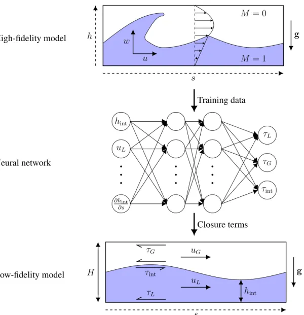
Our approach is shown schematically in Figure 1. We have a 2D high-fidelity model for channel flow, with horizontal and vertical velocity componentsuandw, being functions of the coordinatessandh. The low-fidelity model is 1D and as such only knows velocitiesuLanduG,

that they are only functions ofs(as is the interface heighthint). From the 2D high-fidelity field

results we calculate these averaged quantities and their corresponding stresses. These represent inputs and desired outputs to a neural network, respectively, between which the neural network is given the task to find a relation. The resulting functions can be fed as closure terms to the low-fidelity model. High-fidelity model h s u w M = 1 M = 0 g Neural network Training data Closure terms ∂hint ∂s

..

.

..

.

..

.

Figure 1: An outline of the approach for learning closure terms from high-fidelity simulations.

2.1 High-fidelity model

The high-fidelity model that we use to generate the training data is the open source code Gerris [33, 34]. It is based on the one-fluid formulation for multiphase flow. This entails the solution of the Navier-Stokes equations for incompressible flow:

∇·u= 0, (1) ∂u ∂t +u·∇u= 1 ρ −∇p+∇· µ∇u+µ(∇u)T+g, (2)

with velocity field u = u(s, h, t) and pressure field p = p(s, h, t) encompassing the entire domain, gravitational accelerationg, densityρ, and viscosityµ(see Figure 1).

Gerris discretizes these equations spatially with a finite volume method on a colocated grid, with central interpolation and the Van Leer generalized minmod limiter withθ = 2for the face-centered gradient calculation. We do not make use of Gerris’ capability to adaptively refine the grid at different levels.

For temporal discretization Gerris uses a second order projection method [11], in which a multilevel Gauss-Seidel iterative method is used to solve the pressure Poisson equation. The velocity advection term is discretized according to the second order unsplit upwind scheme of Bell et al. [4], and for the diffusion term a Crank-Nicolson discretization is employed.

In the one-fluid approach for multiphase flow, the densityρand viscosityµare functions of the spatial coordinates, via a marker functionM =M(s, h, t):

ρ=ρ(M), µ=µ(M).

This marker functionM, typically 1 in the liquid and 0 in the gas, is advected by the velocity field. We make theassumption of sharp interfaces[43, p. 22] and disregard phase transition, so that the advection of the marker function can be described by

DM Dt =

∂M

∂t +u·∇M = 0. (3)

Gerris advects the marker function numerically using the volume-of-fluid (VOF) method. In the VOF method [19], the marker function is averaged over the grid cells to define the color function Ci = 1 Vi Z Vi MdV. (4)

The color function is a function which gives the volume fraction of the reference fluid in a grid cell. The material properties in grid cells i can then be expressed as functions of this color function. We use the expressions

ρi =Ciρ1+ (1−Ci)ρ0, (5) µi = Ci µ1 + 1−Ci µ0 −1 . (6)

with ρ1 and µ1 the density and viscosity of the fluid indicated by M = 1 and ρ0 and µ0 the

fluid indicated by M = 0. For the viscosity we do not use an arithmetic mean but rather the harmonic mean [14], which improves the accuracy of the velocities and stresses at a flat, horizontal interface.

Prior to the actual advection step, the interface is reconstructed from the color function using the PLIC method [47]. The color function is then advected geometrically by the velocity field.

We use most of the standard Gerris settings, except that we lower the tolerance of the pro-jection steps from1·10−3_to1·10−6_{. After a convergence study, the grid spacing∆s= ∆his}

set toH/64, and the time step is set so that the maximum value of

CFL = |u|∆t

∆s (7)

anywhere in the simulation is 0.8. However, there is an additional constraint that in mixed VOF cells the maximum value should be 0.5. We do not filter the color function (i.e. averaging over multiple cells), to keep the interface relatively sharp.

We choose the one-fluid formulation for multiphase flow with the VOF interface advec-tion method for its conservative properties, its simplicity, and its similarity to our low-fidelity model. Alternative interface advection methods for the one-fluid formulation of multiphase flow include the front tracking [46] and level-set methods [39], but these are not naturally mass conservative.

2.2 Low-fidelity model

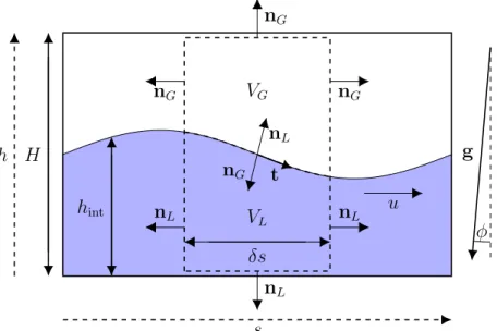
Our low-fidelity model is known as the 1D two-fluid model. It is obtained by considering control volumes in a channel, separate for liquid and gas, as pictured in Figure 2. The limitδs→

0is taken, while the control volumes fill the full channel height. Since we do not consider phase change, the velocities are continuous at the interface. The stresses tangential to the interface, the shear stresses, must be continuous, and since we assume hydrostatic balance (without surface tension) the pressure should be continuous along the vertical direction, as well as the stresses along the vertical direction.

s δs H h hint nG nG nL nL nL nG VG VL u g φ nL nG t

Figure 2: Two small (δs H) control volumes for two-phase pipe flow. At the top and bottom the control volume is bounded by impenetrable no-slip boundaries. The interface separates the two control volumes.

We obtain one equation for mass balance and one for momentum balance for each fluid. In channel flow these take the following form:

∂ ∂t(ρLhint) + ∂ ∂s(ρLuLhint) = 0, (8a) ∂ ∂t(ρG(H−hint)) + ∂ ∂s(ρGuG(H−hint)) = 0, (8b) ∂ ∂t(ρLuLhint) + ∂ ∂s ρLu 2 Lhint = − ∂pint ∂s hint+LGL+FL −ρLhintgsin (φ), (8c) ∂ ∂t(ρGuG(H−hint)) + ∂ ∂s ρGu 2 G(H−hint) = − ∂pint ∂s (H−hint) +LGG+FG −ρG(H−hint)gsin (φ), (8d)

withuLanduGthe averaged velocities of the liquid and gas respectively,ρLandρGlikewise for

the densities,hintthe interface height,pintthe interfacial pressure, andφthe channel inclination.

Here the stresses are bundled into closure terms

FL =τL−τint, FG=τG+τint, (9)

and the level gradient terms represent

LGL =− ∂ ∂s 1 2ρLgcos (φ)h 2 int , LGG= ∂ ∂s 1 2ρGgcos (φ) (H−hint) 2 . (10)

The equations are of the same form as those for pipe flow in circular cross-sections, but with different relations between the cross-sections, perimeters, and interface height (see e.g. [36]).

In this research the ‘Rosa’ code developed by Sanderse et al. [35, 36, 37] is employed for solving the incompressible form of (8).

The code discretizes the equations using a finite volume method on a staggered grid. This allows for a strong and straightforward coupling between pressure and velocity. Interpolation is needed for the convective scheme: here we employ a central interpolation, which ensures second order spatial accuracy.

After the system is discretized spatially, the time stepping is considered. We use the constraint-consistent time integration framework for the incompressible two-fluid model presented in [36], with the three-stage, third order strong-stability preserving Runge-Kutta method referenced in [37], which follows Gottlieb et al. [17].

2.3 Closure terms

The liquid wall stressτL, gas wall stressτG, and interfacial stressτint, which appear in (9),

represent the stresses acting in the streamwise direction:

τ = (τ ·n)·ˆs, (11)

with τ the stress tensor andˆs the unit vector along the s-axis. Accounting for the no-slip boundary conditions, assuming hydrostatic balance and horizontal length scales far larger than the vertical length scale, they are related to the velocity profile via

τL = −µL ∂u ∂h h↓0 , τG = µG ∂u ∂h h↑H , τint= −µG ∂u ∂h h↓hint = µL ∂u ∂h h↑hint , (12) in whichx ↑ y and x ↓ y are limits from below and from above respectively (see [10] for a more detailed discussion).

These stresses are a priori unknown in the 1D two-fluid model, since in this model the ve-locities are not resolved in the transverse direction, meaning that the stresses cannot be cal-culated according to (12). Conventionally, steady state experiments are employed to correlate the stresses to the averaged quantities through the steady state balance, essentially implying a streamwise and temporally averaged description of the flow. This yields relations of the form1

τL, τG, τint =f(hint, uL, uG, ρL, ρG, µL, µG, H), (13)

1_{Expressions for the stresses based on the body forces as opposed to the averaged velocities do not close the}

in which all the variables on the right-hand sideareknown in the 1D two-fluid model.

Many experiments are needed to obtain good relations, and therefore it may be difficult to find closure terms in the literature which generalize well to the case at hand. Furthermore, when considering wavy flow, with this method of generation of closure terms only the averaged (positive) effect of waves on the interfacial friction can be taken into account; local effects are averaged out.

For the strongly simplified case of laminar, flat interface, fully developed, steady channel flow, Ullmann et al. [45] have derived analytical solutions for the stresses of the form (13). They are given by

τL =− 1 2fLρLuL|uL|F ∗ L, τG=− 1 2fGρGuG|uG|F ∗ G, τint=− 1 2fGρG(uG−uL)|uG|F ∗ int,G, (14) with friction factors

fL = 3 2 16 ReL, fG= 3 2 16 ReG, (15)

depending on Reynolds numbers

ReL = ρL|uL|DL µL

, ReG= ρG|uG|DG µG

, (16)

based on hydraulic diameters

DL = 2hint, DG= 2(H−hint). (17) F_L∗andF_G∗ are the two-phase correction factors for the wall friction:

F_L∗ = 1 + 1₂uG_u L h µL µG uL uG H−hint hint −1 i 1 + µL µG H−hint hint , F_G∗ = 1 + 1_2uuL G h µG µL uG uL hint H−hint −1 i 1 + µG µL hint H−hint , (18)

andF_int,G∗ that for the interfacial friction:

F_int,G∗ = 1 1 + µG µL hint H−hint . (19)

These closure terms form a reference, with which we benchmark our solvers for the case of steady flow, and to which we compare the new neural network closure terms.

2.4 Closure term limitations

By using closure relations of the form (13), we introduce a fundamental limitation. The averaged velocities cannot be translated back uniquely to velocity profiles, the slopes of which determine the stresses; information is lost in the averaging process. The consequence of this uniqueness problem is that for collections of very different velocity profiles, with the same averaged velocities, the closure relations will predict the same stresses, while the actual stresses can in reality be very different. In most of the literature [2, 5, 12, 15, 20, 40, 44] the analysis is therefore limited to fully developed steady state flow, for which the stressesareuniquely related to the averaged velocities.

There is a second limitation to the degree to which the low-fidelity model can be made to reproduce results of the high-fidelity model in this framework. Closure terms of the form (13)

are introduced as source terms in the low-fidelity model, and cannot be expected to resolve the entire difference in dynamics introduced by the averaging process and the associated assump-tions. The difference between the dynamics of the high- and low-fidelity models, in absence of friction (equivalent to taking the homogeneous part of the equations for the two-fluid model at zero inclination), can be illustrated by performing a linear stability analysis of the two models. Results of this are shown in Figure 3, based on the parameters from Table 1.

Figure 3: Dispersion relationsω(k)withk = 2π/λ, for the 1D two-fluid model without friction terms [22], and for inviscid 2D potential flow [29]. The parameters are given in Table 1, with the steady state solution given in Table 2.

Table 1: Test case parameters.

Parameter Symbol Value Units

Background pressure gradient ∂p/∂s −1 kg m−2s−2 Liquid density ρL 998 kg m−3 Gas density ρG 1.2 kg m−3

Channel height H 0.01 m

Initial interface height hint 0.3H m

Liquid viscosity µL 1.002·10−3 kg m−1s−1 Gas viscosity µG 1.82·10−5 kg m−1s−1 Acceleration of gravity g 9.81 m s−2

Pipe inclination φ 0 degrees

With the analytical solution given by [6] and [45], the corresponding averaged velocities and stresses (for the steady state) can be calculated. These are given in Table 2.

It is observed that the dispersion relation of the 1D model only converges to the dispersion relation of the 2D model at large wavelengths. The cross-sectional averaging of the equations, and the associated assumption of hydrostatic balance, implicitly implies the long wavelength assumption [30].

Table 2: Test case steady state solution, for the parameters given in Table 1.

Parameter Symbol Value Units Averaged liquid velocity uL 0.00818 m s−1 Averaged gas velocity uG 0.232 m s−1 Liquid wall stress τL −0.00646 kg m−1s−2 Gas wall stress τG −0.00354 kg m−1s−2 Interfacial stress τint −0.00346 kg m−1s−2 Liquid Reynolds number ReL 48.9

-Gas Reynolds number ReG 214 -Liquid Froude number FrL 0.00114 -Gas Froude number FrG 0.391

-2.5 Stress extraction

By extracting stresses from high-fidelity simulations via (12), itispossible to consider local and unsteady effects. We can take any position along thes-axis in the simulations and calculate the stresses, and the corresponding averaged variablesuL, uG, hint, at that point. We can

cal-culate additional, local, quantities, which are not defined in a streamwise averaged description — the streamwise derivatives of the averaged variables — and relate these to the stresses as well. Since we can extract the averaged variables and stresses at any point in time in the un-steady simulations, the same holds for temporal derivatives. Because we use a neural network, such new inputs can easily be added to the closure relations, without prior information on the complex relation between them and the stresses.

The stresses are determined practically by fitting cubic splines to the velocity profiles of the liquid and gas separately and taking their analytical derivatives. For the final determination of the interfacial stress, the stresses at the interface as calculated from the liquid and gas profiles are averaged. For more details, see [10].

3 NEURAL NETWORKS

A neural network is used to construct a relation of the form (13), using the high-fidelity model data. For laminar steady state flow the analytical solution can be used to train the neural network instead of the high-fidelity solution (since they are equal). This simple case, for which conventional closure terms are exact, is used to tune the neural network hyper-parameters (in subsection 3.1 and subsection 3.2). Afterwards (in subsection 3.3 and subsection 3.4), the tuned neural network is applied to the more difficult case of unsteady, wavy flow.

3.1 Neural network settings

The network is a multilayer perceptron network (MLP), implemented in the MATLAB Deep Learning Toolbox [41]. It is tuned mainly by comparison of training data error and validation data error as measured by a mean squared error cost function

C = 1 N N X i=1 (yi−y_bi)2, (20)

whereyiis the data for a set of input variablesiandybiis the model prediction for these inputs.

The result is a network with 4 hidden layers with 18 nodes each, each with a hyperbolic tangent activation function, and no regularization term in the cost function (given the size of our training data set). The network is trained using the Levenberg-Marquardt training algorithm [18], an efficient algorithm for smaller networks. A small percentage of the training data (15%) is taken apart and not used for the training; the optimization is stopped if the error on this validation data does not decrease. The training inputs and outputs are mapped to the range

[−1,1](the same translation and multiplication is later applied to unseen data).

We tested the effect of random initialization via the Nguyen-Widrow algorithm [31] and found that different random initializations yield very similar final values of the validation data error. We also verified the convergence of the training and validation errors with increasing amounts of data. These results are available in [10].

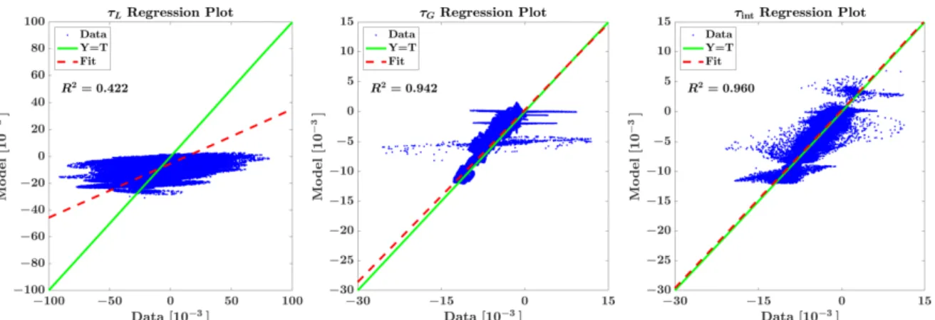
3.2 Performance of networks trained on steady state data

Training the network with steady state data is useful for the network tuning. However, Fig-ure 4 shows that networks trained on steady state data have little predictive capacity for stresses found in wavy unsteady simulations. On the horizontal axis stress values observed in high fi-delity simulations are set out, and on the vertical axis the neural network predictions for the samehint,uL,uG, ... are given. We show the squared correlation coefficient

R2 = 1− PN i=1(byi−yl,i) 2 PN i=1 b yi−(1/N) PN i=1byi 2, (21)

with a range between 0 and 1. In this definition, y_bi is the model prediction. We construct a

linear fit of the model predictiony_bi as a function of the data and call ityl. The valueyl,i is the

value of the linear fit at the data pointyi, corresponding to predictiony_bi.

Figure 4: Regression plots forτL,τG, andτintwith a neural network trained on steady state data as the model, tested on the wavy unsteady high-fidelity simulation data.

The poor performance shown in Figure 4, particularly for the strongly oscillatory liquid stress, could have been expected, as the analytical stresses with which we train the network are derived for steady state flow, while the actual flow is wavy unsteady. Similar poor results are observed when using the analytical stresses as the model directly. This motivates training on unsteady data.

3.3 Generation of wavy unsteady data

We consider 2D channel flow with periodic boundaries left and right under a constant body force in the form of a background pressure gradient ∂p/∂s. No-slip boundary conditions are applied at the top and bottom walls. A sine wave perturbation with wavelengthλand amplitude

∆bhintis applied to the interface between liquid and gas.

We generate data by running the high fidelity code Gerris 60 times, with varying input pa-rameters randomly selected from the ranges given in Table 3. The papa-rameters are selected from these ranges using Latin Hypercube Sampling [28], ensuring a space-filling sampling, without repetition of parameter values. The material properties, channel height, and the channel in-clination are kept at the values given in Table 1. This limits the required amount of (costly) simulations, while allowing practical application to an unsteady flow in a specified pipe and with specified fluids.

The wavelength of the perturbation is fixed atλ=L= 0.12 m, whereLis the length of the domain.

Table 3: The ranges of the parameters of the unsteady high fidelity simulations used as training data.

Initialization hint[H] ∂p/∂s[Pa/m] ∆bh_int[H] Number of simulations zero wavy [0.05,0.95] [0,−3] [0.00,0.04] 30

developed wavy [0.05,0.95] [0,−3] [0.00,0.04] 30

The simulations are initialized from two different initial conditions: • ‘zero wavy’: the velocities in the entire domain are zero,

• ‘developed wavy’: the velocities are initialized at their (flat interface) steady state values (determined analytically [6]),

and then run fromt= 0tot = 10seconds. With these initial conditions and the given parame-ters, we get slowly traveling standing waves (see Figure 9), initially approximated by

∆hint(s, t) = 2∆bhintcos(ks−δωt) cos(ω0t). (22)

These waves are formed as the superposition of two waves traveling in the opposite direction with wave velocities

c1 =

ω0+δω

k , c2 =

−ω0+δω

k , (23)

withδω ω0 due to the small Froude numbers (see Table 2). Later, nonlinear and damping

effects become important; in most cases the waves are largely damped out att= 10.

Note that the parameter ranges in Table 3 are chosen such that the perturbations damp out in time, avoiding a transition to (near-) slug flow and problems of ill-posedness in the 1D two-fluid model (see e.g. [7]).

3.4 Neural network training

At each time step and at each grid point along s the quantities given in (13) are extracted from the Gerris simulations, yielding many data points, which may not all provide distinct information. The networks are therefore trained on small random subsets of the data.

• ‘zero wavy net’: networks trained on data with the ‘zero wavy’ initial condition.

• ‘developed wavy net’: networks trained on data with the ‘developed wavy’ initial condi-tion.

• ‘zero + developed wavy net’: networks trained on a combination of the data with the ‘zero wavy’ initial condition and with the ‘developed wavy’ initial condition.

Per item in the above list, we sample the data with replacement to get five different data sets, each a small percentage of the total data set2_{. We train (randomly initialized) networks on each}

of these subsets of the data. The final prediction for the stresses is obtained by averaging the predictions of each of the five networks, for a given set of inputs. This averaging procedure is called ‘bagging’ and has been shown to improve accuracy for learning algorithms sensitive to changes in the training data [9]. This technique was also employed by Ma et al. [27].

An extra input is added compared to those given by equation (13): the interface slope

∂hint/∂s. The interfacial slope can easily be added to the neural network as an input. This input

does not fit in conventional closure terms which are calculated for the fully developed steady state, since it is a locally defined variable3. If fully developed flow is assumed, or similarly the effect of the wavy interface is averaged out over a length of pipe (as is done by e.g. Andritsos and Hanratty [2]), the average interface slope will be zero (for a flow with a wavy perturbation) and cannot be used to differentiate stresses at different phases of the wavy perturbation.

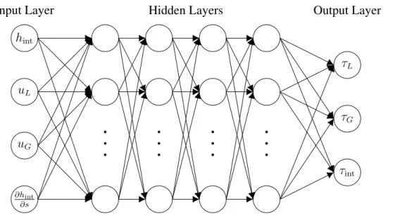
With this addition, and the given selection of variable parameters, the neural network takes the form shown in Figure 5.

Input Layer ∂hint ∂s uG uL hint Hidden Layers

..

.

..

.

..

.

..

.

Figure 5: A schematic of the neural network trained in subsection 3.4, and tested in section 4, with four variable inputs, four hidden layers (with 18 nodes per layer), and three outputs.

2_{The percentages of the data sets taken per individual training are 5% for the ‘zero wavy net’ and ‘developed}

wavy net’, and 10% for the ‘zero + developed wavy net’

3_{An exception is Brauner and Moalem Maron [8], who modified conventional closure terms (based on Taitel}

and Dukler [40]) to add a dependency of the interfacial stress on the interfacial slope, by matching experimentally observed and theoretically calculated stability boundaries (the latter of which depends on the closure terms). The advantage of our method is that the interfacial slope is included in the correlation from the beginning, in the same straightforward manner as the other inputs.

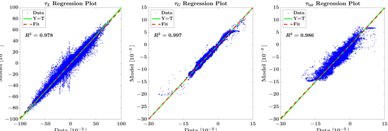
Resulting regression plots for a ‘zero + developed wavy net’ are shown in Figure 6. The correlation is satisfactory, considering the variation in flow patterns found in the data. The influence of the extra input parameter∂hint/∂sis illustrated by comparison of Figure 6 to

Fig-ure 7, where in the latter figFig-ure results are shown if this parameter is left out. Apparently the interfacial slope is an important piece of information for the determination of the stresses. This parameter allows the stress prediction to vary based on the wave’s amplitude and local phase, and allows distinction between fully developed and unsteady flow, alleviating the uniqueness issue discussed in subsection 2.4.

Figure 6: Regression plots for a neural network trained on the data combined for both initial conditions of Table 3 (‘zero + developed wavy net’).

Figure 7: Regression plots for a neural network trained on the data combined for both initial conditions of Table 3 (‘zero + developed wavy net’) excluding the interface slope∂hint/∂sas an input.

4 RESULTS

The true test of the learned closure terms lies in their application to the low-fidelity model Rosa, and comparison of the resulting predictions to high-fidelity model Gerris predictions (presumed to be the truth). At each stage in the Runge-Kutta time integration scheme, the variables as given in (5) are fed to the trained neural networks to arrive at values for the stresses

τL, τG, and τint. The current MATLAB shallow neural network implementation significantly

slows down the Rosa code simulations, compared to when the analytical closure relations (14) are used.

In order to be able to compare Gerris and Rosa results (with different grid resolutions) quan-titatively, cubic splines of the variables of interest are constructed, along the horizontal axis. The resultings-dependent Gerris result att =ti isyi = yi(s), withybi = byi(s)the

correspond-ing Rosa result. We compute characteristic values yc for each variable of interest, based on

analytical solutions for laminar single phase flow. Table 4 shows the following relative error measure for the difference between Gerris and Rosa results, termed the ‘normalized averaged error’ (NAE): NAE = 1 NT NT X i=1 s 1 L Z L s=0 yi−y_bi yc 2 ds. (24)

The parameterNT is the total number of time steps andLis the length of the domain.

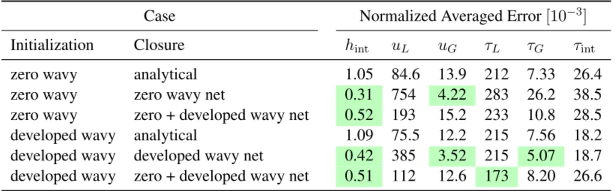
This error is shown for simulations initialized from different initial conditions, and using different closure terms. Analytical closure terms (14) are tested alongside closure terms learned from the wavy unsteady data of Table 3, using neural networks. Where the neural network assisted error is smaller than the analytical closure error, the error value is highlighted green in Table 4.

Table 4: Normalized averaged errors (24) between Gerris and Rosa simulations, for different variables of interest. Results are given for Gerris and Rosa simulations starting from different initial conditions, with the Rosa simulations using either analytical or neural network closure terms. Where the neural network closure terms outperform the analytical closure terms (for the same initialization), the result is highlighted in green.

Case Normalized Averaged Error[10−3] Initialization Closure hint uL uG τL τG τint zero wavy analytical 1.05 84.6 13.9 212 7.33 26.4 zero wavy zero wavy net 0.31 754 4.22 283 26.2 38.5 zero wavy zero + developed wavy net 0.52 193 15.2 233 10.8 28.5 developed wavy analytical 1.09 75.5 12.2 215 7.56 18.2 developed wavy developed wavy net 0.42 385 3.52 215 5.07 18.7 developed wavy zero + developed wavy net 0.51 112 12.6 173 8.20 26.6

Overall, with error measure (24), the results with neural network closure terms do not show a significant improvement, except perhaps for the interface height. However, this error measure is crude and does not show how well the wave dynamics are reproduced.

We therefore study the values of hint, uL, uG, τL, τG, τint as a function of time in Rosa

simulations for the test case given by Table 1, at a point at the center of the domain (s = 0.06 m) (see Figure 8). The scale and form of the oscillations are captured better when using the neural network closure terms; the wave damping behavior corresponds better to the high-fidelity simulations. The interface height in the entire domain is shown in Figure 9 for a number of time instants, with the shown Rosa simulations employing the neural network closure terms. The problem with the analytical closure terms is highlighted in Figure 10, in which the same simulation results are shown for later time instants (with the analytical closure). The waves acquire a sharp wavefront, in the wake of which small spurious waves are formed. These effects are unphysical and are not observed in the Gerris simulations. The neural network closure terms do not suffer from these spurious effects, probably due to their better damping behavior.

(a) Analytical closure. (b) Zero + developed wavy net closure.

(c) Analytical closure. (d) Zero + developed wavy net closure.

(e) Analytical closure. (f) Zero + developed wavy net closure.

Figure 8: Evolution in time of the velocities, stresses and interface height at the center of the domain. Initialized with the ‘developed wavy’ initial condition.

Figure 9: Evolution in time of the interface between liquid and gas throughout the domain, zoomed in at the interface (H = 0.01 m). Rosa results with a ‘developed wavy’ initialization and ‘zero + developed wavy net’ closure.

Figure 10: Evolution in time of the interface between liquid and gas throughout the domain, zoomed in at the interface (H = 0.01 m). Rosa results with a ‘developed wavy’ initialization and analytical closure.

Training the neural network on unsteady simulation data allows the closure terms to capture the unsteady (damping) behavior, differentiating them from conventional steady state closure terms (including those closure terms that consider the streamwise averaged effect of a wavy interface). The addition of the extra closure input parameter∂hint/∂s, allows the closure terms

to apply the learned differences between steady state and unsteady flow patterns. By providing information on the wave amplitude and local phase, this input parameter enables distinction between steady state flow and increasingly unsteady flow during application in Rosa. This allows the closure terms to provide different results for different phases of the wave damping process. Similarly, the closure terms can produce different stresses at different points along the wave (beyond the distinction made possible by the small differences in interface height and averaged velocities).

One of the problems still visible in Figure 8 is a discrepancy in the steady state gas velocity; this can be solved by further grid refinement of the Gerris simulations.

The remaining main difference between Gerris simulations and Rosa simulations using neu-ral network closure terms is a discrepancy in the wave speed. The wave speed of the Rosa simulations is slightly higher than that of the Gerris simulations, so that the two slowly drift out of phase. This difference in wave speed between Gerris and Rosa simulations can be explained by the fact that a discrepancy between the models remains that cannot be solved via modeling the closure terms (see subsection 2.4). The inviscid dispersion relations for the test case, plotted in Figure 3, indeed show a higher wave speed for the 1D model than for the 2D model.

5 CONCLUSION & OUTLOOK

In this work, we have explored a new approach based on neural networks to solve the long-standing closure problem for stratified multiphase flow in channels. We have trained neural networks on high fidelity simulation data to learn closure terms for the wall and interfacial stresses in a low fidelity model; the 1D two-fluid model for stratified channel flow. An important novelty in our work is the inclusion of the streamwise derivative of the interface height as a feature in the neural network. With this addition, the dynamic wave-damping behavior of high-fidelity simulations was reproduced better than with the conventional (steady state) set of closure terms available in literature [45].

With the proposed framework, closure terms can be constructed for specific flow regimes and duct geometries, as long as high-fidelity simulations are available. The addition of extra inputs to the closure relations, which is straightforward in this framework, alleviates their inherent uniqueness problem. An example of possible extra inputs, besides the interface slope, are the spatial and temporal derivatives of the velocities.

We note that, even with a highly accurate closure model for the stresses, the 1D model will generally not exactly reproduce the 2D results, because the stresses are not the only source of discrepancy between the 1D and 2D model. In principle, it might be possible to eliminate these discrepancies by modeling the difference between high- and low-fidelity model predic-tions directly, and adjusting the low-fidelity model accordingly. But this approach would be less physical, so that it might not generalize as well.

In the future we aim to improve the framework through closer inspection of the structure of the learned closure terms, and possibly through the inclusion of physical constraints in the network structure. This will open the door to more challenging cases, such as the prediction of slug flow.

REFERENCES

[1] A. Alizadehdakhel, M. Rahimi, J. Sanjari, and A. A. Alsairafi. CFD and artificial neural network modeling of two-phase flow pressure drop. International Communications in Heat and Mass Transfer, 36:850–856, 2009.

[2] N. Andritsos and T. J. Hanratty. Influence of interfacial waves in stratified gas-liquid flows.AIChE Journal, 33:444–454, 1987.

[3] D. Barnea and Y. Taitel. Interfacial and structural stability of separated flow. Interna-tional Journal of Multiphase Flow, 20:387–414, 1994.

[4] J. B. Bell, P. Colella, and H. M. Glaz. A second-order projection method for the in-compressible Navier-Stokes equations. Journal of Computational Physics, 85:257–283, 1989.

[5] D. Biberg. A mathematical model for two-phase stratified turbulent duct flow.Multiphase Science and Technology, 19, 2007.

[6] D. Biberg and G. Halvorsen. Wall and interfacial shear stress in pressure driven two-phase laminar stratified pipe flow. International Journal of Multiphase Flow, 26:1645– 1673, 2000.

[7] N. Brauner and D. Moalem Maron. Stability analysis of stratified liquid-liquid flow. In-ternational Journal of Multiphase Flow, 18:103–121, 1992.

[8] N. Brauner and D. Moalem Maron. The role of interfacial shear modelling in predicting the stability of stratified two-phase flow.Chemical Engineering Science, 48:2867–2879, 1993.

[9] L. Breiman. Bagging predictors.Machine Learning, 24:123–140, 1996.

[10] J. F. H. Buist. Machine Learning for Closure Models in Multiphase-Flow Applications. Master’s thesis, Eindhoven University of Technology, 2019.

[11] A. J. Chorin. On the convergence of discrete approximations to the Navier-Stokes equa-tions.Mathematics of Computation, 23:341–353, 1969.

[12] S. W. Churchill. Friction factor equation spans all fluid flow regimes. Chemical Engi-neering, 84:91–92, 1977.

[13] N. Coutris, J. M. Delhaye, and R. Nakach. Two-phase flow modelling: the closure issue for a two-layer flow.International Journal of Multiphase Flow, 15:977–983, 1989. [14] A. V. Coward, Y. Y. Renardy, M. Renardy, and J. R. Richards. Temporal evolution of

peri-odic disturbances in two-layer Couette flow.Journal of Computational Physics, 132:346– 361, 1997.

[15] M. Espedal. An Experimental Investigation of Stratified Two-Phase Pipe Flow at Small Inclinations. PhD thesis, Norwegian University of Science and Technology, 1998. [16] M. Gamahara and Y. Hattori. Searching for turbulence models by artificial neural

net-work.Physical Review Fluids, 2:054604, 2017.

[17] S. Gottlieb, C.-W. Shu, and E. Tadmor. Strong stability-preserving high-order time dis-cretization methods.SIAM Review, 43:89–112, 2001.

[18] M. T. Hagan and M. B. Menhaj. Training feedforward networks with the Marquardt algorithm.IEEE Transactions on Neural Networks, 5:989–993, 1994.

[19] C. W. Hirt and B. D. Nichols. Volume of fluid (VOF) method for the dynamics of free boundaries.Journal of Computational Physics, 39:201–225, 1981.

[20] J. E. Kowalski. Wall and interfacial shear stress in stratified flow in a horizontal pipe. AIChE Journal, 33:274–281, 1987.

[21] B. I. Krasnopolsky and A. A. Lukyanov. A conservative fully implicit algorithm for pre-dicting slug flows.Journal of Computational Physics, 355:597–619, 2018.

[22] J. Liao, R. Mei, and J. F. Klausner. A study on the numerical stability of the two-fluid model near ill-posedness.International Journal of Multiphase Flow, 34:1067–1087, 2008.

[23] J. Ling, A. Kurzawski, and J. Templeton. Reynolds averaged turbulence modelling using deep neural networks with embedded invariance. Journal of Fluid Mechanics, 807:155– 166, 2016.

[24] C. Lu, S. Sambasivan, A. Kapahi, and H. S. Udaykumar. Multi-scale modeling of shock interaction with a cloud of particles using an artificial neural network for model repre-sentation.Procedia IUTAM, 3:25–52, 2012.

[25] C. Lu. Artificial Neural Network for Behavior Learning from Meso-Scale Simulations, Application to Multi-Scale Multimaterial Flows. Master’s thesis, University of Iowa, 2010.

[26] M. Ma, J. Lu, and G. Tryggvason. Using statistical learning to close two-fluid multiphase flow equations for a simple bubbly system.Physics of Fluids, 27:092101, 2015.

[27] M. Ma, J. Lu, and G. Tryggvason. Using statistical learning to close two-fluid multiphase flow equations for bubbly flows in vertical channels.International Journal of Multiphase Flow, 85:336–347, 2016.

[28] M. D. McKay, R. J. Beckman, and W. J. Conover. A comparison of three methods for selecting values of input variables in the analysis of output from a computer code. Tech-nometrics, 21:239–245, 1979.

[29] L. M. Milne-Thomson. Theoretical Hydrodynamics. Macmillan, London, 4th edition, 1962.

[30] M. Montini. Closure Relations of the One-Dimensional Two-Fluid Model for the Simu-lation of Slug Flows. PhD thesis, Imperial College London, 2011.

[31] D. Nguyen and B. Widrow. Improving the learning speed of 2-layer neural networks by choosing initial values of the adaptive weights. In Proceedings of the 1990 IJCNN International Joint Conference on Neural Networks, volume 3, pages 21–26, San Diego, CA, USA. IEEE, 1990.

[32] R. E. Osgouei, A. M. Ozbayoglu, E. M. Ozbayoglu, E. Yuksel, and A. Eresen. Pressure drop estimation in horizontal annuli for liquid–gas 2 phase flow: Comparison of mecha-nistic models and computational intelligence techniques.Computers & Fluids, 112:108– 115, 2015.

[33] S. Popinet. An accurate adaptive solver for surface-tension-driven interfacial flows. Jour-nal of ComputatioJour-nal Physics, 228:5838–5866, 2009.

[34] S. Popinet. Gerris: a tree-based adaptive solver for the incompressible Euler equations in complex geometries.Journal of Computational Physics, 190:572–600, 2003.

[35] B. Sanderse, S. Misra, and S. Dubinkina. Numerical simulation of roll waves in pipelines using the two-fluid model. In Proceedings of the 11th North American Conference on Multiphase Production Technology, pages 373–386, Banff, Canada, 2018.

[36] B. Sanderse and A. E. P. Veldman. Constraint-consistent Runge–Kutta methods for one-dimensional incompressible multiphase flow.Journal of Computational Physics, 384:170– 199, 2019.

[37] B. Sanderse, I. E. Smith, and M. H. W. Hendrix. Analysis of time integration methods for the compressible two-fluid model for pipe flow simulations.International Journal of Multiphase Flow, 95:155–174, 2017.

[38] F. Sarghini, G. de Felice, and S. Santini. Neural networks based subgrid scale modeling in large eddy simulations.Computers & Fluids, 32:97–108, 2003.

[39] M. Sussman, P. Smereka, and S. Osher. A level set approach for computing solutions to incompressible two-phase flow.Journal of Computational Physics, 114:146–159, 1994. [40] Y. Taitel and A. E. Dukler. A model for predicting flow regime transitions in horizontal

and near horizontal gas-liquid flow.AIChE Journal, 22:47–55, 1976.

[41] The MathWorks, Inc. MATLAB Documentation - Deep Learning Toolbox. 2019. URL:

https://nl.mathworks.com/help/deeplearning/index.html (visited on 02/03/2019).

[42] B. D. Tracey, K. Duraisamy, and J. J. Alonso. A machine learning strategy to assist turbulence model development. In Proceedings of the 53rd AIAA Aerospace Sciences Meeting, Kissimmee, Florida. American Institute of Aeronautics and Astronautics, 2015. [43] G. Tryggvason, R. Scardovelli, and S. Zaleski. Direct Numerical Simulations of

Gas-Liquid Multiphase Flows. Cambridge University Press, 2011.

[44] A. Ullmann and N. Brauner. Closure relations for two-fluid models for two-phase strati-fied smooth and stratistrati-fied wavy flows.International Journal of Multiphase Flow, 32:82– 105, 2006.

[45] A. Ullmann, A. Goldstein, M. Zamir, and N. Brauner. Closure relations for the shear stresses in two-fluid models for laminar stratified flow. International Journal of Multi-phase Flow, 30:877–900, 2004.

[46] S. O. Unverdi and G. Tryggvason. A front-tracking method for viscous, incompressible, multi-fluid flows.Journal of Computational Physics, 100:25–37, 1992.

[47] D. L. Youngs. Time-dependent multi-material flow with large fluid distortion. In K. W. Morton and M. J. Baines, editors, Numerical Methods for Fluid Dynamics. Academic Press, 1982.