2016
Applications of Optimization Under Uncertainty
Methods on Power System Planning Problems
Bokan Chen
Iowa State University
Follow this and additional works at:
https://lib.dr.iastate.edu/etd
Part of the
Industrial Engineering Commons
This Dissertation is brought to you for free and open access by the Iowa State University Capstones, Theses and Dissertations at Iowa State University Digital Repository. It has been accepted for inclusion in Graduate Theses and Dissertations by an authorized administrator of Iowa State University Digital Repository. For more information, please [email protected].
Recommended Citation
Chen, Bokan, "Applications of Optimization Under Uncertainty Methods on Power System Planning Problems" (2016).Graduate Theses and Dissertations. 16511.
planning problems
by
Bokan Chen
A dissertation submitted to the graduate faculty in partial fulfillment of the requirements for the degree of
DOCTOR OF PHILOSOPHY
Major: Industrial Engineering
Program of Study Committee: Lizhi Wang, Major Professor
Mingyi Hong James D. McCalley
Sarah M. Ryan Lily Wang
Iowa State University Ames, Iowa
2016
TABLE OF CONTENTS LIST OF TABLES . . . v LIST OF FIGURES . . . vi ACKNOWLEDGEMENTS . . . vii ABSTRACT . . . viii CHAPTER 1. INTRODUCTION . . . 1 1.1 Overview . . . 1
1.2 Optimization Under Uncertainty Methods . . . 1
1.3 Transmission Expansion Planning . . . 3
1.4 Power System Resiliency Planning . . . 5
CHAPTER 2. ROBUST OPTIMIZATION FOR TRANSMISSION EXPAN-SION PLANNING: MINIMAX COST VS. MINIMAX REGRET . . . 7
2.1 Nomenclature . . . 8 2.2 Introduction . . . 9 2.3 Model Formulation . . . 14 2.3.1 Deterministic model . . . 14 2.3.2 The MMC model . . . 16 2.3.3 The MMR model . . . 16 2.4 Algorithm Development . . . 17
2.4.1 The master problem for the MMC model . . . 18
2.4.2 The subproblem for the MMC model . . . 18
2.4.3 Algorithm for the MMC model . . . 19
2.5 Case Study . . . 22
2.6 Conclusion . . . 27
CHAPTER 3. ROBUST TRANSMISSION PLANNING UNDER UNCER-TAIN GENERATION INVESTMENT AND RETIREMENT . . . 29
3.1 Nomenclature . . . 30
3.2 Introduction . . . 31
3.3 Model Formulation . . . 35
3.4 Solution Methods . . . 38
3.4.1 Master problem and subproblem . . . 39
3.4.2 Solving the subproblem . . . 40
3.4.3 Algorithm . . . 42
3.5 Case Study . . . 43
3.6 Conclusion . . . 51
CHAPTER 4. A STOCHASTIC PROGRAMMING FRAMEWORK FOR OPTIMAL DISTRIBUTION NETWORK HARDENING . . . 54
4.1 Nomenclature . . . 55
4.2 Introduction . . . 56
4.3 Model Formulation . . . 60
4.4 Solution Method . . . 62
4.4.1 Sample average approximation . . . 62
4.4.2 Single replication procedure . . . 63
4.4.3 L-shaped method . . . 64
4.4.4 Greedy search heuristic . . . 66
4.5 Case Study . . . 67
4.5.1 Scenario generation . . . 67
4.5.2 Experiment results . . . 69
4.5.3 Solution validation . . . 71
CHAPTER 5. CONCLUSION AND DISCUSSION . . . 75
LIST OF TABLES
Table 2.1 Motivating Example for the Minimax Regret Model . . . 12
Table 2.2 Motivating Example for the Minimax Cost Model . . . 12
Table 2.3 Generation Parameters . . . 22
Table 2.4 Candidate Line Parameters . . . 23
Table 2.5 Number of Iterations for Each Instance . . . 24
Table 2.6 Expansion plan of the MMC approach . . . 25
Table 2.7 Expansion plan of the MMR approach . . . 26
Table 2.8 Comparison of the MMC, MMR and Deterministic Solutions for Uncer-tainty Set U1. . . 26
Table 2.9 Comparison of the MMC, MMR and Deterministic Solutions for Uncer-tainty Set U2. . . 27
Table 2.10 Investment and Operational costs for scenarios ($m) . . . 27
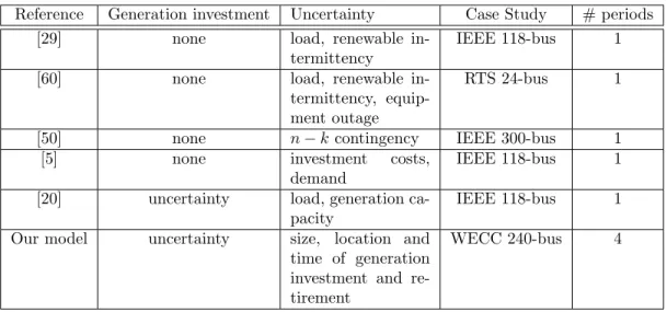
Table 3.1 Comparison with other robust optimization transmission planning mod-els in the literature . . . 35
Table 4.1 Hardening costs . . . 70
Table 4.2 Avergae Load Shedding under different budgets . . . 72
LIST OF FIGURES
Figure 3.1 Summary of the robust optimization modeling framework . . . 36
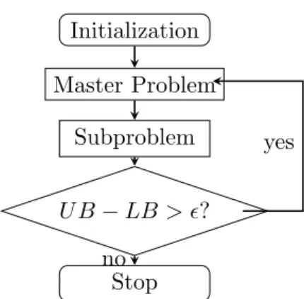
Figure 3.2 Flow chart of the decomposition algorithm . . . 43
Figure 3.3 WECC 240-bus test system topology from [52] . . . 44
Figure 3.4 Visualization of the transmission planning problem . . . 47
Figure 3.5 Six transmission plans. . . 49
Figure 3.6 Twelve scenarios. The label ‘W1’ is for the worst-case scenario for Plan 1, ‘B2’ for the best-case scenario for Plan 2, and so on. . . 50
Figure 3.7 Performance of six plans. The horizontal axis of each sub-graph is the 20-year planning horizon, containing four discrete 5-year periods. . . . 52
Figure 4.1 Typical Scenario . . . 69
Figure 4.2 IEEE 33-Bus Test Case . . . 70
Figure 4.3 24-Hour Load Multiplier . . . 71
Figure 4.4 Hardening Plan (Budget = 7m$) . . . 72
ACKNOWLEDGEMENTS
I would like to express my profound gratitude towards those people who helped me with various aspects of conducting research and the writing of this dissertation. First and foremost, I would like to thank my advisor Dr. Lizhi Wang for his guidance, patience and support through-out my PhD study. He is a great teacher who not only taught me the fundamental technical skills in operations research, but also guided me towards conducting research. He provided me with his insights, inspiration and encouragement to help me complete this dissertation. I could not have done this without him.
I would also like to thank my committee members: Dr. Mingyi Hong, Dr. James D. McCalley, Dr. Sarah M. Ryan and Dr. Li Wang for their tremendous help. I appreciate their time and effort in reading this dissertation and their helpful comments in improving this work. In addition, I would like to express my gratitude towards Dr. Jianhui Wang from Argonne National Laboratory for his effort and contribution to this work. His advice and input to my research is invaluable. Needless to say, I am solely responsible for any errors that this dissertation might contain.
Last but not least, I would like to thank my friends and colleagues for their companionships. They make the office a fun place to be. I enjoyed our discussions on life, the universe, and everything.
ABSTRACT
This dissertation consists of two published journal paper, both on transmission expansion planning, and a report on distribution network hardening.
We first discuss our studies of two optimization criteria for the transmission planning prob-lem with a simplified representation of load and the forecast generation investment additions within the robust optimization paradigm. The objective is to determine either the minimum of the maximum investment requirement or the maximum regret with all sources of uncertainty explicitly represented. In this way, transmission planners can determine optimal planning de-cisions that are robust against all sources of uncertainty. We use a two layer algorithm to solve the resulting trilevel optimization problems. We also construct a new robust transmission planning model that considers generation investment more realistically to improve the quan-tification and visualization of uncertainty and the impacts of environmental policies. With this model, we can explore the effect of uncertainty in both the size and the location of can-didate generation additions. The corresponding algorithm we develop takes advantage of the structural characteristics of the model so as to obtain a computationally efficient methodology. The two robust optimization tools provide new capabilities to transmission planners for the development of strategies that explicitly account for various sources of uncertainty.
We illustrate the application of the two optimization models and solution schemes on a set of representative case studies. These studies give a good idea of the usefulness of these tools and show their practical worth in the assessment of “what if” cases. We compare the performance of the minimax cost approach and the minimax regret approach under different characterizations of uncertain parameters. In addition, we also present extensive numerical studies on an IEEE 118-bus test system and the WECC 240-bus system to illustrate the effectiveness of the proposed decision support methods. The case study results are particularly useful to understand the impacts of each individual investment plan on the power system’s
overall transmission adequacy in meeting the demand of the trade with the power output units without violation of the physical limits of the grid.
In the report on distribution network hardening, a two-stage stochastic optimization model is proposed. Transmission and distribution networks are essential infrastructures to modern society. In the United States alone, there are there are more than 200,000 miles of high voltage transmission lines and numerous distribution lines. The power network spans the whole country. Such vast networks are vulnerable to disruptions caused by natural disasters. Hardening of distribution lines could significantly reduce the impact of natural disasters on the operation of power systems. However, due to the limited budget, it is impossible to upgrade the whole power network. Thus, intelligent allocation of resources is crucial. Optimal allocation of limited budget between different hardening methods on different distribution lines is explored.
CHAPTER 1. INTRODUCTION
1.1 Overview
In this proposal, I present research during my PhD career. My research has been focusing on the application of optimization under uncertainty techniques on problems arise in power systems. Two main topics are covered in this proposal:
(1) The application of robust optimization on transmission expansion planning problems.
(2) The application of stochastic programming in the planning of the hardening strategies of
distribution networks.
This chapter presents a brief introduction to the discussed topics. Chapter 2 and Chapter 3
contains my two papers on robust transmission expansion planning. My report for the third
part of my research— power system resiliency planning, is presented in Chapter4.
1.2 Optimization Under Uncertainty Methods
For many optimization problems, the input parameters of a developed model are assumed to be deterministic. However, in more and more real world applications, this is no longer true. In such cases, the optimal solution obtained by a deterministic model may not be optimal or even feasible. As such, methods of optimization under uncertainty have been garnering a lot of attention in fields including power system. Currently, two of the most popular ways to deal with uncertainty in mathematical programming is robust optimization and stochastic programming. Both methods have been widely applied in power system [61].
The problems solved in this dissertation all fall roughly into the category of two-stage optimization models. The two stages refer to the two decision making process before and after
uncertainties are observed. If no uncertainty is considered, and supposebdenote the sources of
uncertainty,xdenote the first-stage decisions that should be made before uncertainty realization
andy denote the second-stage decisions that can only be made after uncertainty is observed, a
typical deterministic linear programming model can be formulated as follows:
minx,y c>x+d>y (1.1)
s.t. x∈ X (1.2)
Ax+By≤¯b (1.3)
where ¯b represent the mean of the uncertainty parameters.
In robust optimization, it is usually assumed that uncertain parameters in an optimization model can be described by polyhedral sets [11, 25]. Such uncertainty sets can be constructed by using information like the lower and upper bounds of the uncertain parameters. Then the objective value under the worst-case scenario is optimized. Although robust optimization is relatively conservative and can lead to worse performance in average, it can guarantee the feasibility of the optimal solution and provide a bound on the objective value. Typically, robust optimization can be formulated as follows:
min
x∈X c
>x+ max
b∈U miny∈Y(x,b)d>y (1.4)
whereU is the uncertainty set andY(x, b) ={y|Ax+By≤b}is the feasible set for second-stage decision variables. From this formulation we can see that the uncertainty parameter is treated as a variable to identify the worst-case scenario.
On the other hand, stochastic programming assumes the accurate probability distribution of the uncertain parameters can be obtained. The expected value of the objective function over the aforementioned distribution is optimized. Scenarios are usually generated based on the probability distributions to represent the uncertain data. In order to guarantee feasibility and good performance, a reasonable number of scenarios should be generated, which leads to large problem size. Many algorithms can be applied to solve such large-scale optimization prob-lems, including Benders’ decomposition and progressive hedging [43]. Stochastic programming models can be formulated as follows:
min x∈§ +E[Q(x, ˜b)] (1.5) where Q(x, b) = min c>y (1.6) s.t. Ax+By≤˜b (1.7)
Both robust optimization and stochastic programming have their strengths and weaknesses. In this dissertation they are applied to two different types of problems based on the requirements of the applications.
1.3 Transmission Expansion Planning
Transmission planning (TP) is one of the key decision processes in the power system produc-tion pipeline. Electricity transmission networks are responsible for reliably and economically delivering power from generators to consumers. Thus, a robust and resilient transmission net-work is essential to the operation of power systems for decades to come. Good transmission investments have many benefits, including satisfying increasing demand, promoting social wel-fare, improving system reliability and resource adequacy, etc. Transmission planning is also very challenging due to various sources of uncertainty that planners need to consider. Besides uncertainty sources, such as demand variations and renewable energy intermittency faced by system operators in short-term scheduling, planners also need to take into consideration uncer-tainty of policy changes, technological advancements and natural disasters [61]. Such sources of uncertainty cannot be characterized in terms of analytical probability distributions. For example, to cope with challenges of climate change, the power generation industry is facing increasing pressure to reduce greenhouse gas emissions. In addition, a large amount of coal plants are anticipated to retire in response to the implementation of the EPA clean power plan [19], and their replacement in part by gas-fired plants. Moreover, after the restructuring of the power system, certain behavior by generation companies introduces additional uncertainty in power system planning in general and TP in particular. However, research on the impacts of
uncertain future generation developments on TP is scarce in the decentralized decision making environment in competitive market. As such, the study of this topic is warranted.
Conventional transmission planning methodologies are typically deterministic and some make use of ad-hoc approaches to deal with uncertainty. These methodologies have served the industry relatively well in the vertically-structured industry. Present realities brought about, by the open access regime and the advent of competitive electricity markets, increased wind and solar resource outputs. Their highly time varying, uncertain and intermittent patterns, combined with the more dynamically varying and uncertain loads and a world-ranging envi-ronmental policy initiative have resulted in a more volatile utilization of transmission facilities. Critically needed is the improved planning methodologies that can effectively accommodate the realities of the new environment. Transmission planning, by its very nature, is subject to a wide range of sources of uncertainty that must be taken into account. The new regime indicates many additional sources of uncertainty and numerous complications that must be considered.
Over a 10-20 year planning horizon, major sources of uncertainty faced by transmission planning decision makers include load growth, fuel costs, climate change events, atmospheric conditions, variable generation outputs, generation expansion/retirement events, regulatory and legislative developments, technology breakthroughs and market outcomes. When the im-pacts of transmission plans are assessed, such studies must be carefully performed with the explicit representation of the sources of uncertainty, in light of the overarching consequences on the power system. These sources of uncertainty may be classified into two categories: aleatoric and epistemic sources of uncertainty. Sources of aleatoric uncertainty cannot be replaced by more accurate measurements but they can be statistically quantified. For instance, the coinci-dental uncertainty with respect to the electrical system state and network topological state can be both probabilistically and stochastically modeled and quantified if the relevant sets of input are made available. On the other hand, sources of epistemic uncertainty are due to information we may in principle know, but do not in actual practice. Often, such sources are also called sources of systematic uncertainty. For instance, it is hard to assign meaningful probabilities to sources of uncertainty associated with government policies, technology breakthroughs, and investment in renewable energy generation.
Electricity demand is expected to grow continually and steadily for decades to come. In the EIA Annual Energy Outlook 2013, forecasts indicate that electricity consumption will increase by 28% from 2011 to 2040 at an average of about 1% per annum rate[24]. To accommodate such growth in electricity demand, new capacity of electricity generation must be built at a pace that meets or exceeds the growth of demand and retirement of old generators to maintain power system reliability. The additional demand and capacity require commensurate transmission capacity.
With the additional sources of uncertainty and complications facing transmission planners and the need to accommodate increasing demand as well as more variable generation capacity, there is a critical need for new TP methodologies that can address the aforementioned concerns. The first two papers in this dissertation address this problem.
1.4 Power System Resiliency Planning
In addition to transmission expansion planning, resilience planning is also an important step to improve the security of power systems. In the United States, there are more than 200,000 miles of high voltage transmission lines and numerous distribution lines that span the whole country. Such vast networks are vulnerable to disruptions caused by natural disasters including seismic activities and extreme climate events. Due to climate change, frequency of natural disasters such as floods, droughts, hurricanes and other weather activities is expected to rise. Improving power system security and resilience not only would reduce the probability of disrupted operations, but also could be instrumental to the recovery of communities from catastrophes.
Resilience is defined as a combination of two capabilities: the inherent ability of a system to cope with disruption with the networks topology and redundancies, and its ability to recover from disruptions. Both abilities need to be considered in order to improve system resilience. One illustrative example is underground power lines, even though they are invulnerable to many natural disasters including hurricanes, wild fires and snow storms, they are more difficult to repair. In a region prone to earthquakes, even with low probability, undergrounding power lines may not be a good choice.
According to [54], hardening is one of the most effective approaches to improve the resilience
of power grids. Methods of hardening include upgrading power poles and structures with
stronger materials, vegetation management and undergrounding utility lines. In addition to hardening, investment can also be devoted to reduce response time and expedite infrastructure recovery after the occurrence of disruptions. Options include response planning, training of personnel and improved outage notification ability. Such investments are usually constrained by a limited budget. Thus, hardening of the entire grid simultaneously could be prohibitively expensive and therefore is unrealistic. It is crucial to allocate the limited resources to the most vulnerable components or to the power lines with the largest impact if affected. The last paper uses stochastic programming to solve the budget allocation problem in power system hardening.
CHAPTER 2. ROBUST OPTIMIZATION FOR TRANSMISSION EXPANSION PLANNING: MINIMAX COST VS. MINIMAX REGRET
Published inIEEE Transactions on Power Systems
Bokan Chen, Jianhui Wang, Lizhi Wang, Yanyi He and Zhaoyu Wang
Abstract
Due to the long planning horizon, transmission expansion planning is typically subjected to a lot of uncertainties including load growth, renewable energy penetration, policy changes, etc. In addition, deregulation of the power industry and pressure from climate change introduced new sources of uncertainties on the generation side of the system. Generation expansion and retirement become highly uncertain as well. Some of the uncertainties do not have probability distributions, making it difficult to use stochastic programming. Techniques like robust op-timization that do not require a probability distribution became desirable. To address these challenges, we study two optimization criteria for the transmission expansion planning prob-lem under the robust optimization paradigm, where the maximum cost and maximum regret of the expansion plan over all uncertainties are minimized respectively. With these models, our objective is to make planning decisions that are robust against all scenarios. We use a two layer algorithm to solve the resulting tri-level optimization problems. Then, in our case studies, we compare the performance of the minimax cost approach and the minimax regret approach under different characterizations of uncertainties.
2.1 Nomenclature Sets and indices
U The polyhedron uncertainty set of demand and new generation capacity profile
I Set of nodes
L Set of existing transmission lines
N Set of candidate transmission lines
T Set of years in the planning horizon
M Set of load blocks
K Set of technology types
Parameters
Pi,k,t Capacity of existing generator of technologyk at nodeiat timet
cTij,t Cost of building the new transmission lineij at time t
cLi,t Cost of load curtailment at nodeiat time t
cPi,k,t Cost of power production of technologykat node i
fk,t,mC Average capacity factor of generation technologykat year tload block m
Fijmax The maximum power flow on transmission lineij
Bij Susceptance of transmission lineij
M A big constant used to linearize the power flow constraint
¯
di,t,m The average amount of demand at yeart load blockm at node i ¯
PN
i,k,t The average amount of generation expansion of technologykat node iat timet
θmin The lower bound of voltage angles
θmax The upper bound of voltage angles
λ Market interest rate (Inflation included)
Pi,k,tN,min Minimum amount of new generation at a node
Pi,k,tN,max Maximum amount of new generation at a node
PN,min Lower bound on the total amount of generation at all the nodes
Decision Variables
xij Binary variables indicating whether a transmission line is built
Pi,k,tN The amount of new generation capacity of technologykat nodeiat timet. Pi,k,tN is negative in the case of power plant retirement
fij,t,m Power flow from nodeito node j at yeart load blockm
pi,k,t,m Power production of technology kat node iat yeart load blockm
ri,t,m The amount of load shedding at nodeiat year tload block m
θi,t,m Voltage angle at nodeiat year tload block m
di,t,m Demand at year tload block mat node i
2.2 Introduction
Transmission expansion planning is very challenging due to various uncertainties planners need to consider. Besides typical high-frequency uncertainties including demand variations and renewable energy intermittency faced by system operators in short-term scheduling, plan-ners also need to take into consideration low-frequency uncertain events like policy changes, technological advancements, natural disasters, etc. [61]. Such uncertainties cannot be charac-terized by probability distributions. For example, to cope with challenges of climate change, the power generation industry is facing increasing pressure to reduce greenhouse gas emissions. In addition, a large amount of coal plants are anticipated to retire in response to government regulations and fuel price changes [19], replaced partially by gas-fired plants. Many of such retirements could be announced on relative short notice and unexpected by the system oper-ator. Moreover, after the deregulation of the power system, strategic behavior of generation companies in generation expansion becomes an uncertain factor as well.
Currently, the most common practices in dealing with uncertainties in optimization include stochastic programming and robust optimization. In stochastic programming, scenarios are generated based on a certain probability distribution of the uncertain data. The weighted sum of the total cost under different scenarios is usually optimized. Stochastic programming has been successfully applied to power system capacity expansion planning problems. In [59, 36, 44, 26], uncertainties including load prediction inaccuracies, transmission line and generator outages,
generation and transmission line capacity factors are considered. All of those uncertainties can be described by probability distributions and can be effectively modeled with stochastic programming techniques. However, most of those works only focus on uncertainties in the operation phase and do not address uncertainties in the planning phase. The reason is that it is difficult to obtain probability distributions of the non-random [17] or epistemic uncertainties caused by factors including policy changes, investment behavior of market players, etc. In this paper, besides load uncertainty, we also take into consideration uncertain generation expansion behavior of generating companies and coal power plants retirement.
As an alternative tool to address uncertainties, robust optimization [11, 25, 14] can avoid some of the difficulties arising from stochastic programming approaches. With robust optimiza-tion, uncertainty is described by parametric sets, which contain an infinite number of scenarios. Such uncertainty sets can be constructed with information like the lower and upper bounds of a random variable, which are much easier to derive than probability distributions. This approach can identify a set of decisions that is robust under the worst-case scenario contained in the uncertainty sets, which is desirable in planning problems where reliability is important. The conservativeness of the solution can be adjusted by changing the uncertainty sets [13], de-pending on how much uncertainty is desired to capture. Robust optimization has been applied
to many problems in power systems. In [62], robust unit commitment with the n−ksecurity
criterion is studied. The problem is then reformulated into a single-level problem with the help of dual variables. In [12, 32], the two-stage robust unit commitment problems under uncer-tainty are studied. Both papers propose to use Bender’s Decomposition to solve the problem. A similar model is used in [74] where demand response is considered. A robust minimax regret model is proposed in [31] to solve the unit commitment problem under uncertainty. However, all those works study operation problems. In long term power system planning problems where more uncertainties need to be considered, application of robust optimization is limited. In [29], a robust transmission expansion planning model is proposed considering load and generation uncertainty. Bender’s decomposition is also used.
In this paper, we propose two robust optimization models to address two main sources of uncertainty: load and generation expansion behavior of generating companies. Two criteria,
minimax cost (MMC) and minimax regret (MMR), are used as the objective of our models. The MMC criterion has been used widely in robust optimization applications [12]. The MMR criterion is considered in [31] for the unit commitment problem. In comparison with the MMC criterion, it is concluded that MMR outperforms MMC for certain unit commitment problems. However, the same conclusion may not apply to transmission expansion planning problems due to the different structures of such problems. In [46], regret is considered as one of the objectives in a multi-objective optimization framework. It is applied to handle non-random uncertainties in [23, 7]. Both criteria use the performance of a decision under the worst possible scenario as the objective for optimization, but their main difference is how the “worst scenario” is defined. The MMC criterion focuses on the cost associated with a decision under a scenario, so the scenario that results in the highest cost is identified as the worst scenario. On the other hand, the MMR criterion defines the worst scenario as the one that leads to the highest regret for
the decision maker. For a given decision d0 and a given scenario s0, the regret is the highest
potential cost savings had the decision maker known that scenarios0 would occur and made a
decision accordingly. More rigorously,
R(d0, s0) =C(d0, s0)−min d∈DC(d, s
0),
whereC(d0, s0) is the cost associated with d0 and s0,D is the set of all feasible decisions, and
R(d0, s0) is the regret associated withd0 and s0. Using these notations, the MMC and MMR
criteria can be respectively formulated as
min d∈D max s∈U C(d, s) and min d∈D max s∈U R(d, s) = min d∈D max s∈U C(d, s)−min d0∈DC(d 0, s) .
We use two simple examples in Tables 2.1 and 2.2to demonstrate the differences between
MMC and MMR. In the first example, under MMC, D2 is the optimal decision because its
worst scenario cost, $8, is lower than that ofD1,$9. Under MMR,D1 is the optimal decision
is that since scenario S1 is a “bad” scenario anyway because D1 and D2 both lead to higher
costs in S1 thanS2, the difference between the costs associated with the two decisions, which
is the regret, may provide more information for decision making than the absolute value of the
cost itself. In the second example, decision D3 is obviously a bad choice because of its high
Table 2.1 Motivating Example for the Minimax Regret Model
Cost / Regret Decision D1 DecisionD2
ScenarioS1 $9 / $1 $8 /$0
ScenarioS2 $2 / $0 $7 /$5
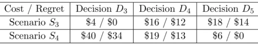
cost in scenario S4. Decision D5 will be selected under MMC because its worst cost, $18, is
lower than that of D3, $40, and D4, $19. Under MMR, decision D4 will be selected since its
worst-case regret is$13 while the regret ofD5 is$14. We argue the MMC solutionD5 is better
in this example because it is only slightly worse than the MMR decision D4 in terms of regret
in scenarioS3 only because of the existence of decisionD3, which cannot be selected anyways,
but has a much lower cost in scenario S4.
Table 2.2 Motivating Example for the Minimax Cost Model
Cost / Regret DecisionD3 Decision D4 DecisionD5
Scenario S3 $4 /$0 $16 /$12 $18 /$14
Scenario S4 $40 /$34 $19 /$13 $6 /$0
From the previous two examples, we can see that there are no clear cut answers as to which criterion is superior. Each of them has advantages and disadvantages. The examples above can shed some light on which criterion may perform better in what situations. In the first example, both decisions perform better in one scenario and worse in the other. In this case, it makes sense to use MMR as the criterion because the MMC criterion is too conservative and does not consider non-extreme scenarios. On the other hand, in the second example, there exists a very risky decision that performs well under one scenario and extremely poorly under the other. In a planning problem where risks should be controlled, such decisions are usually not desirable, but they may affect the maximum regret of other decisions and distort the final decision.
and operation stages of the transmission expansion planning problem very well. They can be formulated as special cases of trilevel optimization problems. However, due to their non-linear, non-convex structure, they are very difficult to solve. In previous researches [12, 32], the authors use Bender’s decomposition to reformulate the problem into a master problem
and a bilinear subproblem, which is then solved with outer approximation. However, the
outer approximation approach cannot handle the binary variables in the subproblem when the MMR criterion is used. In [31], statistical upper bounds are used to complement the outer approximation approach. We propose a two-layer algorithm where we decompose our problem into a master problem and a bilevel subproblem. The master problem is updated with a branch and cut type procedure, where new constraints and variables are iteratively generated and then solved as a mixed-integer program. This algorithm is a special case of the bilevel optimization algorithm [67]. Similar algorithms are proposed in [74, 73]. It works faster than the traditional Bender’s decomposition approach with the use of primal information instead of dual variables. The subproblem is a mixed-integer bilevel optimization problem, which is more difficult to solve. In [49], the difficulty of solving a bilevel linear optimization program is discussed and several heuristics are proposed. We use the Karush-Kuhn-Tucker (KKT) conditions [15] to reformulate the bilevel problem into a single level problem with complementarity constraints, which is then reformulated into a mixed-integer programming problem [28].
The contribution of this paper can be summarized as follows. Firstly, we propose two robust optimization models that use two criteria to assess decisions. Both load uncertainties and generation expansion uncertainties are considered. Then, effective algorithms are proposed to solve the resulting trilevel optimization problems. Finally, in our case studies, the two models and their corresponding algorithms are tested with a modified IEEE 118-bus test system. We then analyze the results and compare the performances of the expansion plans under different scenarios.
The rest of the paper is structured as follows. Section 2.3 presents the mathematical
formulation of the transmission expansion planning problems. In section 2.4, we present the
trilevel optimization algorithm. Numerical results are presented in section2.5. Finally, section
2.3 Model Formulation
Transmission expansion planning problems are usually modeled as two-stage problems to account for the long planning horizon, where the expansion planning decisions are made in the first stage when there is limited information on uncertain parameters and the operational decisions are made in the second stage after uncertainty realizations are observed. In this section, we first present the deterministic model, and then introduce two robust optimization models under the MMC and MMR criteria.
2.3.1 Deterministic model
In the deterministic model, consideration of uncertainty is avoided by assuming perfect information for all parameters. For example, in the following deterministic model, the load is fixed as ¯dand the new generation capacity is fixed as ¯PN.
minX
ij,t
cTij,txij +
X
i,k,t,m
(1 +λ)t(cPi,k,tpi,k,t,m+cLi,tri,t,m) (2.1) s.t.X k pi,k,t,m+ X j fji,t,m− X j
fij,t,m= ¯di,t,m−ri,t,m,∀i∈ I, t∈ T, m∈ M (2.2)
fij,t,m−Bij(θi,t,m−θj,t,m)−(1−xij)M ≤0,∀ij ∈ N (2.3)
Bij(θi,t,m−θj,t,m)−fij,t,m−(1−xij)M ≤0,∀ij ∈ N (2.4)
fij,t,m =Bij(θi,t,m−θj,t,m),∀ij ∈ L (2.5)
fij,t,m ≤Fijmaxxij,∀ij ∈ N (2.6)
−fij,t,m≤Fijmaxxij,∀ij∈ N (2.7)
fij,t,m ≤Fijmax,∀ij∈ L (2.8)
−fij,t,m≤Fijmax,∀ij ∈ L (2.9)
pi,k,t,m≤fk,t,mC (Pi,k,t+ ¯Pi,k,tN )∀i∈ I, t∈ T, m∈ M, k∈ K (2.10)
θmin≤θi,t,m ≤θmax,∀i∈ I, t∈ T, m∈ M (2.11)
The objective function (2.1) is the transmission capital investment cost and total opera-tional cost (including cost of power production and load shedding) over the planning horizon. This model is a static model, in which the total operational cost over the planning horizon
is estimated by extrapolating from |T | years. A similar approach has been used by several
other related studies [36, 26, 35]. Constraint (2.2) requires that the net influx at a node
should be equal to the net outflow. Constraints (2.3) and (2.4) are equivalent to the equation
fij,t,m =xijBij(θi,t,m−θj,t,m), which is nonlinear and complicates the model. We introduce the
constantM to linearize this equation [35]. Whenxij = 1, then the two constraints are reduced
tofij,t,m =Bij(θi,t,m−θj,t,m), where the value of M does not matter. Whenxij = 0, then we
need to make sure that M is large enough so that no additional constraints are imposed. On
the other hand, ifM is too large, it may cause computational difficulties. In our experiments,
we set it to be ten times the largest value ofFijmax. Equation (2.5) calculates the power flow on existing transmission lines. Constraints (2.6)- (2.9) dictate that the power flow on transmission
lines does not exceed their limits. Constraint (2.10) specifies the generation capacity on each
node. Constraint (2.11) limits the range of phase angles at a node.
To facilitate algorithmic development and simplify the notations, we abstract the determin-istic model as follows:
minx,zc>x+b>z (2.13)
s.t. Ax+C1z≤g1 (2.14)
By¯+C2z≤g2 (2.15)
J z = ¯d (2.16)
In this more concise abstract formulation, we usex to represent the binary variable indicating
whether or not a transmission line should be built,y to represent the amount of new generation
and z to represent operational variables including power production, phase angles, power flow
and load curtailment. Vectorscandbrepresent coefficients of variables in the objective function. Matrices A, B, C1, C2, J are the coefficients of variables in the constraints. Vectors g1, g2 are
the right-hand-side parameters in the constraints. Constraint (2.14) corresponds to equations
2.3.2 The MMC model
In the two-stage MMC model, given the first-stage decisions, the second-stage problem is commonly known as the recourse problem [38], where the optimal operation decisions are identified. The feasible set of the recourse problem is defined as follows:
Z(x, d, y) ={z:C1z≤g1−Ax, C2z≤g2−By, J z=d}
The uncertainty set is defined as
U ={(d, y) :Q1d≤q1, Q2y≤q2}
The matrices Q1, Q2 are the coefficients of d and y in the uncertainty set. Vectors q1, q2 are
the right-hand-side parameters. They can contain information including the lower and upper bounds of the uncertain parameters, the lower and upper bounds of the linear combination of the uncertain parameters, etc. Such information can be obtained from historical data or statistical tests on historical data. In this paper we consider both the uncertainty caused by load forecast and the uncertainty caused by future generation expansion. In addition, other types of uncertainties can be easily plugged into the model without affecting the algorithm.
The MMC model can be formulated as:
min xbinary
c>x+ max
(d,y)∈Uz∈Zmin(x,d,y)b
>z
. (2.17)
2.3.3 The MMR model
Unlike the MMC model, the MMR model aims to minimize the worst-case regret under all possible scenarios. Before presenting the MMR model, we first define the feasible set of the perfect information solutionG(d, y) and the perfect information costG(d, y) as follows:
G(d, y) ={(ˆx,zˆ) :Axˆ+C1zˆ≤g1, C2zˆ≤g2−By, Jzˆ=d}. G(d, y) = min ˆ x,z∈Gˆ (d,y) n c>xˆ+b>zˆo.
We can see that G(d, y) is only dependent on the uncertain parameters (d, y) and can only be known after the uncertainty realizations are observed. We call it the perfect information
solution becauseG(d, y) can only be achieved if perfect information about the uncertainties is
available.
Then we can define the MMR model as follows:
min xbinary c>x+ max (d,y)∈U min z∈Z(x,d,y)b >z−G(d, y) . (2.18)
Comparing the MMC model and MMR model side by side, their similarities are very no-ticeable. The difference between them lies in their definition of the “worst-case scenario”. With the MMC criterion, the worst-case scenario is defined as the scenario with the highest cost, while the MMR criterion defines the worst-case scenario where regret is the highest.
To shed more light on which criterion is more appropriate under different situations, we
can classify scenarios into two categories: regretful vs. regretless. We use xC to denote the
MMC solution and xR to denote the MMR solution. R(x, s) is the regret of decision x under
scenario s. If R(xC, s) ≥ R(xR, s), then we call scenario s a regretful scenario for decision
xC. Otherwise, we say it is regretless. When MMR is used, regret is redistributed among the
scenarios. The regretful ones become less regretful and the costs in the regretless scenarios increase. As an uncertainty set consists of both regretful scenarios and regretless scenarios, it is unpractical to predict accurately which type of scenario will occur in the future. However, the classification of scenarios compares and illustrates the advantages of the MMR and MMC approaches for decision-makers to choose the criterion more appropriately for their specific problem. For example, if they are more confident that regretful scenarios will occur, they can choose the MMR criterion. Otherwise, they may choose the MMC criterion.
2.4 Algorithm Development
In this section, we develop a new trilevel optimization algorithm to solve the two robust optimization problems, which we decompose into two levels: the master problem and the subproblem. We first present the algorithm for the MMC model. This algorithm is then modified for the MMR model. Since we use a cutting plane procedure that does not require
duality information, we can reformulate the sub-problem as a mixed-integer linear programming
problem. In [31], the worst-case scenarios are identified via statistical upper bounds with
Monte Carlo simulation. In contrast, our algorithm provides a theoretical global optimality guarantee to find the worst-case scenarios as the entire problem is solved as a mixed-integer linear programming problem after reformulating the sub-problem.
2.4.1 The master problem for the MMC model
The master problem is designed to provide a relaxation of the MMC model (2.17), in which
the search for the worst-case scenario is restricted to be within a given finite set of scenarios, ΩC = {(di, yi),∀i = 1, ...,|ΩC|}, rather than the complete set of scenarios, U. As such, the
master problem yields a lower bound of the MMC model (2.17). We denote the master problem
asMC(ΩC), and it is formulated as the following single level mixed integer linear program.
min x,ξ,zi c >x+ξ (2.19) s.t. ξ≥b>zi ∀i= 1, . . . ,|ΩC| (2.20) Ax+C1zi≤g1 ∀i= 1, . . . ,|ΩC| (2.21) Byi+C2zi≤g2 ∀i= 1, . . . ,|ΩC| (2.22) J zi=di ∀i= 1, . . . ,|ΩC| (2.23) xbinary. (2.24)
2.4.2 The subproblem for the MMC model
The subproblem is defined as the MMC model (2.17) with a given first-stage decision, x.
As such, the subproblem yields an upper bound of the MMC model (2.17). We denote the
subproblem asSC(x), and it is formulated as the following bilevel linear program.
max
(d,y)∈Uz∈Zmin(x,d,y)b
This model can be further reformulated as the following linear program with complementarity constraints (LPCC). max d,y,z,α,β,γ b >z (2.26) s.t. Q1d≤q1 (2.27) Q2y≤q2 (2.28) 0≤g1−Ax−C1z⊥α≥0 (2.29) 0≤g2−By−C2z⊥β ≥0 (2.30) J z =d (2.31) C1>α+C2>β+J>γ+b= 0 (2.32)
LPCC problems can be solved by several algorithms ([28] Branch-and-Bound, Bender’s, Big-M). The big-M approach [28] was found to be one of the most computationally efficient in our
computational experiments. This approach reformulates (2.26)-(2.32) as the following
mixed-integer linear program (MILP). max d,y,z,α,β,γ,ωb >z (2.33) s.t. Constraints (2.27), (2.28), (2.31), (2.32) (2.34) 0≤g1−Ax−C1z≤M ω1 (2.35) 0≤α≤M(1−ω1) (2.36) 0≤g2−By−C2z≤M ω2 (2.37) 0≤β ≤M(1−ω2) (2.38)
Here, M is a sufficiently large constant (big-M) andω1 and ω2 are auxiliary binary variables
that are introduced to enforce the complementarity conditions in (2.29) and (2.30).
2.4.3 Algorithm for the MMC model
The proposed algorithm for the MMC model, which we call AlgMMC, is an iterative one,
in which the master problem is solved to provide an increasing series of lower bound solutions, and then the subproblem is solved to provide a series of decreasing upper bound solutions using
the solution from the master problem,x, as an input. The input for the master problem,ΩC, is iteratively enriched by the solutions from the subproblem until the gap between the lower and upper bounds falls below a tolerance,. Detailed steps of this algorithm are described as follows:
AlgMMC(c, b, A, B, C1, C2, g1, g2, J, Q1, q1, Q2, q2)
Step 0 : Initialization. CreateΩCthat contains at least one selected scenario. SetLB=−∞,
U B =∞, and k= 1. Go to Step 1.
Step 1 : Update k ← k+ 1. Solve the master problem MC(ΩC) and let (xk, ξk) denote its
optimal solution. Update the lower bound asLB←c>xk+ξk and go to Step 2.
Step 2 : Solve the sub-problemSC(xk) and let (dk, yk, zk) denote its optimal solution. Update ΩC ←ΩC∪ {(dk, yk)}, and U B ←c>xk+b>zk.
Step 3 : IfU B−LB > , go to Step 1; otherwise return (xk, dk, yk, zk) as the optimal solution
to (2.17) and LB as the optimal value.
2.4.4 Algorithm for the MMR model
The MMR model can be solved using a similar algorithmic framework to AlgMMC after the
following simplifying yet equivalent reformulation.
min xbinary c>x+ max (d,y)∈U min z∈Z(x,d,y)b > z−G(d, y) = min xbinary c>x+ max (d,y)∈U min z∈Z(x,d,yb) > z− min (ˆx,zˆ)∈G(d,y) n c>xˆ+b>zˆ o = min xbinary c>x+ max (ˆx,zˆ)∈G(d,y) (d,y)∈U min z∈Z(x,d,y)b >z−(c>xˆ+b>zˆ)
To solve this reformulation of the MMR model, which is structurally similar to the MMC
model (2.17), only slight modifications to the master and sub-problems are required. The
master problem is defined for a different set of input scenarios, ΩR = {(di, yi,xˆi,zˆi),∀i = 1, ...,|ΩR|}, in which the two additional variables, ˆxi and ˆzi, represent the optimal investment
master problem as MR(ΩR), and it is formulated as the following single level mixed integer linear program. min x,ξ,zi c >x+ξ (2.39) s.t.ξ≥b>zi−(c>xˆi+b>zˆi)∀i= 1, . . . ,|ΩR| (2.40) Ax+C1zi≤g1 ∀i= 1, . . . ,|ΩR| (2.41) Byi+C2zi≤g2 ∀i= 1, . . . ,|ΩR| (2.42) J zi =di ∀i= 1, . . . ,|ΩR| (2.43) xbinary. (2.44)
We denote the subproblem as SR(x), and it is formulated as the following bilevel linear
program.
max
(d,y)∈U;(ˆx,zˆ)∈G(d,y)
min z∈Z(x,d,y)b >z−(c>xˆ+b>zˆ) ,
which can be solved using the same big-M approach with the following MILP.
max d,y,z,ˆx,z,α,β,γ,ωˆ b > z−(c>xˆ+b>zˆ) (2.45) s.t. Constraints (2.34)-(2.38) (2.46) Axˆ+C1zˆ≤g1 (2.47) By+C2zˆ≤g2 (2.48) Jzˆ=d (2.49) ˆ x binary. (2.50)
With the new definitions of master and sub-problems, the same algorithm AlgMMC can be
used to solve the MMR model with the following minor modification to Step 2, besides the apparent need to change the superscript “C” to “R”:
Step 2 : Solve the sub-problemSR(xk) and let (dk, yk, zk,xˆk,zˆk) denote its optimal solution. UpdateΩR←ΩR∪ {(dk, yk,xˆk,zˆk)}, andU B ←c>xk+b>zk−(c>xˆk+b>zˆk).
2.5 Case Study
In this section, we present numerical experiments of our model and algorithm on an IEEE 118-bus test system, which consists of 186 transmission lines, 5 wind farms, 5 coal plants, 5 gas plants and 33 loads. The network data is available in [2].
We consider 10 candidate lines. The operation costs are calculated based on the data of 4 load blocks. We consider a planning horizon of 20 years, with the operation cost extrapolated from the cost of year 1. Then the operation cost is assumed to increase at the same rate each
year. The characteristics of generation and candidate lines are summarized in Table 2.3 and
Table 2.4 respectively. In our case study, generation capacity data in the system is set to be
able to satisfy all demand levels if there is no network congestion.
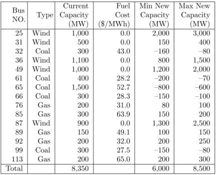
Table 2.3 Generation Parameters
Bus
NO. Type
Current Fuel Min New Max New Capacity Cost Capacity Capacity (MW) ($/MWh) (MW) (MW) 25 Wind 1,000 0.0 2,000 3,000 31 Wind 500 0.0 150 400 32 Coal 300 43.0 –160 –80 36 Wind 1,100 0.0 800 1,500 49 Wind 1,000 0.0 1,200 2,000 61 Coal 400 28.2 –200 –70 65 Coal 1,500 52.7 –800 –600 66 Coal 300 28.3 –150 –100 76 Gas 200 31.0 80 100 85 Gas 300 63.9 150 200 87 Wind 900 0.0 1,300 2,500 89 Gas 150 49.1 100 150 92 Gas 200 32.0 200 250 99 Coal 300 27.5 –150 –80 113 Gas 200 65.0 200 300 Total 8,350 6,000 8,500
Uncertainty in future generation capacity consists of two parts, expansion and retirement. For wind and natural gas fired plants, we set the lower and upper bounds for new capacity. For coal plants, the range of reduced capacity is also provided. We use negative capacity to depict coal retirement. In addition to bounds on individual plants, we also set the lower bound and upper bound on total new generation capacity to control the randomness of the uncertainty set.
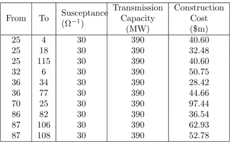
Table 2.4 Candidate Line Parameters From To Susceptance (Ω−1) Transmission Construction Capacity Cost (MW) ($m) 25 4 30 390 40.60 25 18 30 390 32.48 25 115 30 390 40.60 32 6 30 390 50.75 36 34 30 390 28.42 36 77 30 390 44.66 70 25 30 390 97.44 86 82 30 390 36.54 87 106 30 390 62.93 87 108 30 390 52.78
WECC [58]. We generate four instances by changing the uncertainty sets. Their definitions are listed as follows:
U1={0.95 ¯di,t,m≤di,t,m≤1.05 ¯di,t,m (2.51)
Pi,k,tN,min≤Pi,k,tN ≤Pi,k,tN,max (2.52)
PN,min≤X
i,k,t
Pi,k,tN ≤PN,max} (2.53)
U2={0.85 ¯di,t,m≤di,t,m≤1.15 ¯di,t,m (2.54)
Equations(2.52)−(2.53)} (2.55)
U3={0.95 ¯di,t,m≤di,t,m≤1.05 ¯di,t,m (2.56)
[1.25−0.5 sgn(Pi,k,tN,min)]Pi,k,tN,min≤Pi,k,tN
≤[0.75 + 0.5 sgn(Pi,k,tN,max)]Pi,k,tN,max (2.57)
0.75PN,min≤X
i,k,t
Pi,k,tN ≤1.15PN,max} (2.58)
U4={0.85 ¯di,t,m≤di,t,m≤1.15 ¯di,t,m (2.59)
Equations(2.57)−(2.58)} (2.60)
where (Pi,k,tN,min, Pi,k,tN,max) and (PN,min, PN,max) are listed in the last two columns in Table 2.3, with (PN,min, PN,max) in the last row.
The load curtailment cost is set as 2000$/MWh. The interest rate is set as 0.1. The
CPLEX 12.5. The computation time of each instance is around 9 hours. The numbers of
iterations for solving each instance are summarized in Table2.5.
Table 2.5 Number of Iterations for Each Instance
U1 U2 U3 U4
MMC 3 3 2 2
MMR 3 6 2 3
The transmission expansion plans, investment costs and objective values of each criterion
under the four uncertainty sets are summarized in Table 2.6 and 2.7. We then compare the
performances of the MMC solution and the MMR solution under various scenarios in Tables
2.8 and 2.9, where we use Dc, Dr and Dd to denote the optimal MMC solution, the optimal
MMR solution and the optimal deterministic solution. The lower cost and regret between Dc
and Dr are highlighted. The deterministic solution is derived by setting the mean demand as
the load levels and the median of new capacity as the future expansion plans. The scenarios are generated by our algorithms when solving the MMR problems and MMC problems. Each scenario corresponds to an optimal solution to a sub-problem at an iteration of our algorithm and is the worst-case scenario for the first-stage solution obtained at the same iteration. Sce-nariosS1−S3 and S6−S10are generated by solving the MMR problems. Scenarios S4, S5, S11
and S12 are generated when solving the MMC problems. Those scenarios typically have very
high costs or regrets, thus are representative of bad scenarios that robust optimization tries to hedge against. The investment and operational costs of both the MMC and MMR decisions
under the above scenarios are summarized in Table 2.10.
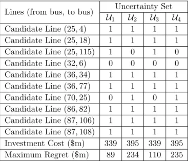
From Table 2.6 and Table 2.7, we can see that as the uncertainty in demand increases,
although the numerical value of the maximum regret and worst-case cost increases, the change in the transmission expansion plan is not very substantial. It means many of the candidate lines are necessary regardless of the demand levels with our unchanged depiction of generation capacity uncertainties. The reason is that those candidate lines connect regions with very high locational marginal price differences due to the presence of large amount of wind energy. On the other hand, when uncertainty in generation expansion is increased, although the total cost also increases, fewer lines are actually built with the MMC criterion. That is because in the
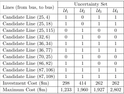
Table 2.6 Expansion plan of the MMC approach
Lines (from bus, to bus) Uncertainty Set
U1 U2 U3 U4 Candidate Line (25,4) 1 0 1 1 Candidate Line (25,18) 1 0 1 1 Candidate Line (25,115) 0 1 0 0 Candidate Line (32,6) 0 1 0 0 Candidate Line (36,34) 1 1 1 1 Candidate Line (36,77) 1 1 1 1 Candidate Line (70,25) 0 1 0 0 Candidate Line (86,82) 1 1 0 0 Candidate Line (87,106) 1 1 1 1 Candidate Line (87,108) 1 1 1 1 Investment Cost ($m) 298 414 262 262 Maximum Cost ($m) 1,233 1,960 1,927 2,802
worst-case scenarios, the system contains less renewable energy capacity and the differences in the locational marginal prices between the otherwise connected regions are not substantial enough to justify new transmission lines. When the MMR criterion is used, however, the final expansion plan does not seem to be sensitive to the change of uncertainty in generation expansion. One possible explanation is that since the MMR criterion does not make decisions only based on the boundary scenarios, it is less sensitive to the changes in uncertainty sets.
From the more detailed comparisons of results from the MMC and MMR approaches in
Tables2.8and 2.9, we can gain more insights about which criterion is more appropriate under
different situations. Both robust optimization solutions outperform the deterministic solution
under most of the scenarios. When the uncertainty set is U1, the MMC solution outperforms
the MMR solution under most of the listed scenarios. When the uncertainty set isU2, on the
other hand, the MMR solution has a lower total cost under more listed scenarios. The solutions
of the cases when the uncertainty sets are U3 and U4 yield similar results. According to our
definition at the end of section2.3, scenariosS2−S5 in Table2.8and scenarioS12in Table2.9
are regretless scenarios for the MMC decision, while scenariosS1andS6−S11are regretful ones.
Which criterion should be used depends on the decision-maker’s perception on the uncertainty sets. In typical regretless scenarios for MMC decisions, there usually exists high demand and
Table 2.7 Expansion plan of the MMR approach
Lines (from bus, to bus) Uncertainty Set
U1 U2 U3 U4 Candidate Line (25,4) 1 1 1 1 Candidate Line (25,18) 1 1 1 1 Candidate Line (25,115) 1 0 1 0 Candidate Line (32,6) 0 0 0 0 Candidate Line (36,34) 1 1 1 1 Candidate Line (36,77) 1 1 1 1 Candidate Line (70,25) 0 1 0 1 Candidate Line (86,82) 1 1 1 1 Candidate Line (87,106) 1 1 1 1 Candidate Line (87,108) 1 1 1 1 Investment Cost ($m) 339 395 339 395 Maximum Regret ($m) 89 234 110 235
Table 2.8 Comparison of the MMC, MMR and Deterministic Solutions for Uncertainty Set
U1 Cost/Regret ($m) Dc Dr Dd ScenarioS1 1,137 / 117 1,109 / 89 1,085 / 65 ScenarioS2 1,039 / 0 1,080 / 41 1,263 / 224 ScenarioS3 803 / 0 844 / 41 1,125 / 422 ScenarioS4 1,126 / 0 1,167 / 41 1,325 / 199 ScenarioS5 1,233 / 27 1,272 / 66 1,367 / 161
low renewable energy penetration. If decision-makers care more about such scenarios or believe they are more likely, then MMC should be used. Otherwise, choosing MMR might be better. Both criteria provide good upper bounds for the total costs under scenarios contained in an uncertainty set. The MMC criterion provides a smaller upper bound with higher average costs while the costs of MMR decisions are lower on average but have higher variability.
From the above results, it is obvious that both the future generation expansion behavior of generation companies and demand uncertainty play important roles in transmission expansion planning. In addition, we can also conclude that both criteria have their merits and can yield relatively reliable expansion plans that guarantee zero curtailment for uncertainty realizations contained in the uncertainty sets. However, depending on the characteristics of uncertainty sets and the preference of decision-makers, they may outperform each other under different
Table 2.9 Comparison of the MMC, MMR and Deterministic Solutions for Uncertainty Set U2 Cost/Regret ($m) Dc Dr Dd Scenario S6 1,730 / 170 1,597 / 37 1,861 / 301 Scenario S7 1,375 / 133 1,354 / 112 1,519 / 277 Scenario S8 1,309 / 497 1,046 / 234 836 / 24 Scenario S9 1,398 / 288 1,266 / 156 1,473 / 363 ScenarioS10 776 / 246 701 / 171 666 / 136 ScenarioS11 1,959 / 201 1,862 / 104 2,082 / 324 ScenarioS12 1,960 / 31 1,962 / 33 2,173 / 244
Table 2.10 Investment and Operational costs for scenarios ($m)
Dc Dr Dc Dr InvestS1−S5 298 339 InvestS6−S12 414 395 OperationS1 839 770 OperationS6 1,316 1,202 OperationS2 741 741 OperationS7 961 959 OperationS3 505 505 OperationS8 895 651 OperationS4 828 828 OperationS9 984 871 OperationS5 935 933 Operation S10 362 306 1 Operation S11 1,545 1,467 1 Operation S12 1,546 1,567
situations. Thus, a comparative analysis of the MMC and MMR criteria can shed more light on better utilization of both approaches.
2.6 Conclusion
In this paper, we propose two robust optimization models for the transmission expansion planning problem under uncertainty, where we take into consideration both the high-frequency uncertainty caused by load forecast errors and the low-frequency uncertainty caused by future generation expansion and retirement. We use two criteria: minimax cost and minimax regret, and compare their performances. The uncertain parameters are described by a polyhedral uncertainty set. With this approach, we can derive an expansion plan that is robust under all scenarios. The resulting models can be formulated as trilevel mixed-integer problems. We use a branch and cut type mechanism to decompose the problem into a master problem and a subproblem. The subproblem generates scenarios and returns them to the master problem
to cut off sub-optimal solutions. The bilevel mixed-integer subproblem is reformulated into a single level mixed-integer-programming problem with the KKT conditions to obtain the global
optimal solution. Our model and algorithm are then tested on an IEEE 118-bus system,
where we compare the results of our MMR and MMC models and analyze their differences. We conclude that the MMR and MMC criteria may outperform each other depending on the uncertainty set and decision-maker’s preference. Interesting topics for future research include developing effective heuristics and parallel computing mechanisms to speed up our algorithms and implementing our algorithms on high performance machines to test larger systems with more candidate lines.
CHAPTER 3. ROBUST TRANSMISSION PLANNING UNDER UNCERTAIN GENERATION INVESTMENT AND RETIREMENT
Published inIEEE Transactions on Power Systems
Bokan Chen and Lizhi Wang
Abstract
Transmission planning is typically faced with a wide range of uncertainty including growth in demand, renewable energy generation and fuel price. The restructuring of the electric power industry, the drive for energy independence and the push for a cleaner environment have led to additional sources of uncertainty in all aspects of power system operations and planning. The more decentralized decision-making implicates uncertainty in future generation investment and retirement of existing units. Such uncertainties are among the biggest challenges in transmis-sion planning in power systems. However, existing approaches in the literature do not fully address this problem. In this paper, we construct a new robust transmission planning model representing generation investment and retirement uncertainty more realistically to improve the quantification and visualization of uncertainty and the impacts of environmental policies. With this model, we can manage the impacts of uncertainty in the time, the size and the lo-cation of candidate generation additions as well as the retirement of units. The corresponding algorithm we develop takes advantage of the structural characteristics of the model so as to obtain a computationally efficient solution methodology. We present an extensive numerical study on the WECC 240-bus system [58] and illustrate the effectiveness of our approach.
3.1 Nomenclature Sets and indices
I Set of nodes,i∈ I
Q Set of all generators (including existing and candidate generators),q∈ Q
W Set of candidate generators,q∈ W
L Set of transmission lines existing before any new investment, (i, j)∈ L
N Set of candidate transmission lines, (i, j)∈ N
T Set of periods in the planning horizon,t∈ T
M Set of load blocks,m∈ M
K Set of generation technology types,k∈ K
R Set of renewable generation technology types,k∈ R
Parameters
Pq,i,k Capacity of generatorq of technologyk at busi
cTi,j,t Cost of building the new transmission line (i, j) at period t
cLi,t Cost of load curtailment at nodei at periodt
cPq,i,k,t Cost of power production by generatorq of technologykat nodeiat periodt Fk,t,mC Average capacity factor of generation technologyk at periodt for load block
m
Fi,jmax Thermal capacity of transmission line (i, j)
Bi,j Susceptance of transmission line (i, j)
M,M0 Big constants used to linearize the power flow constraints and the products
between two variables
di,t,m Demand at node iat periodtfor load block m
θmin The lower bound of voltage angles
θmax The upper bound of voltage angles
λ Cash flow interest rate (with inflation)
Variables
xi,j,t Binary variable indicating whether transmission line (i, j) is built at period t (xi,j,t = 1) or not (xi,j,t= 0)
gq,i,k,t Binary variable indicating whether a generatorq of technology type k exists at busiin periodt(gq,i,k,t= 1) or not (gq,i,k,t= 0)
fi,j,t,m Power flow from nodeito nodej at periodtfor load block m
pq,i,k,t,m Power production by generatorq of technologykat nodeiat periodtfor load
blockm
ri,t,m The amount of load shedding at nodeiat periodtfor load block m
θi,t,m Voltage angle at nodeiat periodtfor load block m
z An aggregate variable representing all dispatch variables, including fij,t,m,
pq,i,k,t,m,ri,t,m, and θi,t,m
CI(x) Net present value of the investment cost
CO(z) Net present value of the operation cost
3.2 Introduction
Transmission planning is one of the key decision processes in the power system production pipeline. Electricity transmission networks are responsible for reliably and economically deliv-ering power from generators to consumers. Thus, a robust and resilient transmission network is essential to the operation of power systems for decades to come. Good transmission invest-ments have many benefits, including satisfying increasing demand, promoting social welfare, improving system reliability and resource adequacy. In addition, in the face of challenges of climate change, the power generation industry is under increasing pressure to reduce its carbon footprint, and to introduce more renewable energy into the power system. Transmission enables a large quantity of renewable energy to be integrated into the power system by bridging the distances between renewable energy resources and load centers.
Transmission planning is very challenging due to the long planning horizon and various sources of uncertainty planners need to consider. Traditionally, planners take into consideration sources of uncertainty such as demand variations and renewable energy intermittency [70,
3], forced outages of transmission lines and generators [40, 18], and transmission capacity factor [45]. Since the restructuring of the power system, generation expansion planning and transmission planning are conducted by separate entities, which makes the future generation investment uncertain to transmission planners. In addition, a large amount of coal plants are anticipated to retire in response to the EPA clean power plan, to be replaced in part by gas-fired plants. Such retirement could be unexpected by system operators. All of the above factors introduce additional sources of uncertainty to the transmission planning process. However, research on the impacts of uncertain future generation developments on transmission planning in the decentralized decision making environment is scarce in the literature.
In existing literature, the most popular methods to manage uncertainty in optimization in-clude stochastic programming and robust optimization. Stochastic programming assumes that the uncertain parameters follow an estimated probability distribution and generates scenarios accordingly. It has been applied to many transmission planning problems [3, 40, 18, 45]. Ryan et al. [61] classify sources of uncertainties in the power system into two categories—high fre-quency and low frefre-quency. Most operational level uncertainties are of high-frefre-quency, whose probability distributions are readily available by utilizing historical data. Low frequencies un-certainties, such as climate change, natural disaster, technology breakthroughs and future gen-eration investment and retirement, cannot be easily characterized by probability distributions. Stochastic programming, with its dependence on probability distributions, is more equipped to deal with high-frequency uncertainties. On the other hand, robust optimization uses paramet-ric sets to describe uncertainty [74, 13], which can contain infinitely many scenarios without specific knowledge of the probability distributions. Therefore, robust optimization can also deal with low-frequency uncertainty. However, the focus in literature has been using robust optimization to ensure feasibility against any operational level high-frequency uncertainty re-alizations. In [29], a robust transmission planning model considering demand and renewable energy uncertainty is proposed. The model is solved by a two-layer Benders’ decomposition algorithm. Ruiz and Conejo [60] propose a similar model with the uncertainty in equipment outages also represented. Robust optimization is also used in [50] with the explicit
in construction costs and demand is considered. The cited references are limited to the man-agement of operational level sources of uncertainty. The impacts of generation investment on transmission planning are usually explored with other methods.
Generation investment in transmission planning is usually studied with three different perspectives—deterministic, stochastic and game theoretic. The references cited in the pre-vious paragraph fall into the deterministic category, which assume generation capacity avail-able in the system to be known information throughout the transmission planning horizon. Stochastic methods include scenario analysis and robust optimization. Similar to stochastic programming, scenario analysis optimizes the average objective among several scenarios with equal weights that represent various sources of uncertainty. However, such scenarios do not
incorporate any information on probability distribution. Munozet al. [52] construct 3 scenarios
based on EIA forecasts and some educated assumptions to describe different policy mandates and fuel costs. Generation investments are determined according to the three scenarios and
are assumed to have the same objective as transmission investments. Buygi et al. [17] study
several cases with different scenarios to explore the effect of low frequency uncertainties. In [42], multi-period scenario trees are constructed to describe the uncertainty in the size, location and types of renewable generation. The disadvantages of this approach is that only a limited number of scenarios are explored. In addition, the constructed scenarios are more of a “big picture” rather than detailed depictions of possible futures. Unlike scenario analysis, robust optimization can describe uncertainty with more details. Two robust transmission planning models with different optimization criteria—minimax cost and minimax regret are proposed in [20]. Demand and generation capacity uncertainty is considered, where generation capacity at specific locations is assumed to be in a polyhedral set. Limited by the way uncertainty is modeled, this work does not explore the impacts of location and time of generation investment and retirement.
In game theoretic models, generation investment is not a source of uncertainty, but the op-timal behavior of generation companies (GENCOs), which can be anticipated based on market condition and the behavior of other players. A trilevel model is proposed in [57]. In the first level transmission investment decisions are made. In the second level, multiple GENCOs make


![Figure 3.3 WECC 240-bus test system topology from [52]](https://thumb-us.123doks.com/thumbv2/123dok_us/10217645.2925616/54.918.209.745.378.778/figure-wecc-bus-test-topology.webp)
