Measuring coherence of computer-assisted likelihood ratio methods

Repositorio Institucional de la Universidad Autónoma de Madrid

https://repositorio.uam.es

Esta es la versión de autor del artículo publicado en:

This is an author produced version of a paper published in: Forensic Science International 249 (2015): 123 – 132 DOI: http://dx.doi.org/10.1016/j.forsciint.2015.01.033

Copyright: © 2015 Elsevier B.V.

El acceso a la versión del editor puede requerir la suscripción del recurso Access to the published version may require subscription

Measuring Coherence of

Computer-Assisted Likelihood Ratio Methods

Rudolf Haraksim*, Daniel Ramos

, Didier Meuwly*, Charles E.H. Berger*

[email protected] (+41 787 11 08 99), [email protected], [email protected], [email protected]

*Netherlands Forensic Institute, Laan van Ypenburg 6, The Hague, Netherlands +_{ATVS – Biometric Recognition Group. Escuela Politecnica Superior. Universidad}

Autonoma de Madrid. C/ Francisco Tomas y Valiente 11. 28049 Madrid, Spain

KEYWORDS: Coherence, Forensic Evidence, Fingermark, Fingerprint, Likelihood Ratio, Validation.

ABSTRACT

Measuring the performance of forensic evaluation methods that compute likelihood ratios (LRs) is relevant for both the development and the validation of such methods. A framework of performance characteristics categorized as primary and secondary is introduced in this study to help achieve such development and validation. Ground-truth labelled fingerprint data is used to assess the performance of an example likelihood ratio method in terms of those performance characteristics. Discrimination, calibration, and especially the coherence of this LR method are assessed as a function of the quantity and quality of the trace fingerprint data. Assessment of the coherence revealed a weakness of the comparison algorithm in the computer-assisted likelihood ratio method used.  

Measuring Coherence of

Computer-Assisted Likelihood Ratio Methods

KEYWORDS: Coherence, Forensic Evidence, Fingermark, Fingerprint, Likelihood Ratio, Validation.

ABSTRACT

Measuring the performance of forensic evaluation methods that compute likelihood ratios (LRs) is relevant for both the development and the validation of such methods. A framework of performance characteristics categorized as primary and secondary is introduced in this study to help achieve such development and validation. Ground-truth labelled fingerprint data is used to assess the performance of an example likelihood ratio method in terms of those performance characteristics. Discrimination, calibration, and especially the coherence of this LR method are assessed as a function of the quantity and quality of the trace fingerprint data. Assessment of the coherence revealed a weakness of the comparison algorithm in the computer-assisted likelihood ratio method used.

*Manuscript (without author details)

1. INTRODUCTION

Forensic research makes progress in the field of evaluation of forensic findings. An increasingly adopted approach [1] uses a logical framework based on Bayes’ Theorem to report forensic evidence in terms of likelihood ratios [1,2]. Computer-assisted LR methods (also referred to simply as LR methods), have been developed to assist the forensic practitioner in his role of forensic evaluator [3,4,5,6,7,8,9]. In these methods pattern recognition algorithms are often used for the feature extraction (analysis), the feature comparison, and statistical models are used for the evaluation of the forensic findings.

In this article the term validation refers to a series of experiments, and the application of a set of performance metrics and validation criteria to demonstrate validity. This is different from Ref. [10], where the term validity was defined as a single metric and equated to accuracy. The specific performance characteristics, performance metrics and validation criteria are used to describe the performance of methods computing LRs and to assess the limits of their validity when used for casework. The LR describes the strength of the evidence, and does not imply a decision by itself. Therefore, the validation of LRs is not the validation of a decision process, but of a description process. We define coherence as a performance characteristic, understood as the ability of a LR method to perform better and to maintain low rates of misleading evidence as some measured parameters influencing quality in the features studied improve, and vice versa. A concrete example is provided when studying and assessing the coherence of a forensic fingermark evaluation method, based on a comparison algorithm of an AFIS (Automated Fingerprint Identification System). When analysing the coherence of the method we hope to observe a LR value increasing with the intrinsic quantity and quality of the information present in the trace data (such as the length of a speech fragment or the number of minutiae in a fingermark).

Forensic service delivery makes progress in the field of quality assurance. Initiatives in the European Network of Forensic Science Institutes (ENFSI) focus on best practices, method validation and service accreditation [11,12]. But because LR methods for forensic evaluation are still very new, the question of their validation has not been addressed yet in the context of quality assurance. Currently, performance characteristics, performance measures, and validation criteria exist to assess analytical forensic methods [13] and human-based methods used for forensic evaluation [14,15]. These approaches are however not suitable for the validation of LR methods developed for forensic evaluation. Such a validation requires

specific performance characteristics, performance measures and validation criteria related to the nature of the LRs and the computation methods involved.

Studying the coherence contributes to describing the performance of the LR method using datasets in which some measurable parameters influencing the strength of the evidence vary. The variation of the length of utterances in forensic automatic speaker recognition and the variation of the number of minutiae in fingermarks are examples of such parameters. Coherence is a highly desirable property of a LR method.

The remainder of this article is structured as follows. The definition of coherence in a set of performance characteristics is presented in Section 2. Section 3 introduces the experimental example for assessment of the coherence of LRs assigned using computer-assisted methods. The different datasets used to measure the performance characteristics are described in Section 4, while the relevance of the use of the datasets and their specificity is described in Section 5. The performance metrics related to the performance characteristics used are introduced in Section 6. Results in terms of coherence of the LR method are presented in Section 7, followed by general discussion and conclusions in Section 8.

Throughout this article we frequently use the terms performance characteristic – a measurable property (or a set of measurable properties) of LRs; and performance metrics – a quantitative description of the performance characteristic. These definitions are ours and the terms may have different meanings in other related works.

2. PERFORMANCE CHARACTERISTICS

Several performance characteristics have been defined to assess the performance of computer-assisted LR methods developed for forensic evaluation. We propose to structure them into primary and secondary performance characteristics. Primary performance characteristics directly measure desirable properties of the LRs. The secondary performance characteristics measure how sensitive primary performance characteristics are to factors like the quantity of information in the data, and to the forensic casework circumstances, such as degraded quality, different technical and temporal conditions related for example to the acquisition of trace and test1 specimens, representativeness of the data, etc.

1 _{In the fingerprint modality the trace usually refers to the fingermark recovered from the crime scene and the}

2.1 Primary performance characteristics

To assess the performance of computer-assisted LR methods, several performance characteristics have been defined recently in forensic evaluation [16]. A very important one is accuracy, defined as the combination of discrimination (discriminating power) and calibration [16,17,18].

• Accuracy is defined as the closeness of agreement between the decision – driven by a LR

computed by a given method – and the ground truth. The LR is accurate if it helps to lead to a decision that is correct2_{. In case of source level inference, the ground truth relates to}

the following pair of propositions:

o Hp: The pair of specimens compared come from the same source (SS) o Hd: The pair of specimens compared come from different sources (DS)

Ground-truth labels are defined as SS (same source) when the LR was calculated for specimens originating from the same source, and as DS (different source) when the LR was calculated for specimens originating from the different sources. If an experimental set of LR values is to be evaluated, and the corresponding ground-truth label of each of the LR values is known, then a given LR value is evaluated as more accurate if it supports the true (known) proposition to a higher degree, and vice-versa.

• Discrimination (or discriminating power) is a property of a set of LRs that allows

distinguishing between the propositions involved. See [16,17] for details.

• Calibration is another property of a set of LRs. Perfect calibration of a set of LRs means

that those LRs can probabilistically be interpreted as the evidential value of the comparison result for either proposition in a Bayesian evaluation framework. Finding a LR = x will be x times more probable under Hp than under Hd (in other words, the LR of

the LR is the LR [19,20]). Under those conditions the LR is exactly as big or small as is warranted by the data. Well-calibrated LRs tend to increase with the discrimination of a given method [16].

2.2 Example factors influencing the primary performance characteristics

2 _{The LR does not imply a decision, but the accuracy measurement is inserted in a decision-theoretical process}

• Quality of the data is a measurable parameter that has no information about the

proposition, but can predict the performance of that comparison. In other words, specimens of high quality to be compared in a forensic case predict good performance of that comparison while low quality samples predict bad performance of a LR method. Examples are the quantity of minutiae in fingerprint comparisons or the signal-to-noise ratio in speaker recognition.

• Quantity3 or amount of data, e.g. the length of a speech fragment, the number of

minutiae in a fingermark, etc.

• Representativeness of the data used to train the LR method for the data used in

operational conditions. The smaller the dataset shift [22] between the two, the more representative the training data is for those in operational conditions.

2.3 Secondary performance characteristics

• Coherence is defined as the ability of the method to yield LRs with better performance

with an increase of the quantity and quality of the information present in the data.

• Generalization is defined as the property of a given method to maintain its performance

under dataset shift. LR method 1 generalizes better than LR method 2 if, under similar conditions of dataset shift in both methods, the performance of method 1 decreases less than the performance of method 2.

• Robustness is the ability of the method to maintain performance when the quantity or

quality of the data decreases. For instance, method 1 is more robust to data sparsity than method 2 if, with decreasing amount of data, the performance of method 1 decreases less than the performance of method 2.

In the next section we present an experimental example to illustrate the measurement of coherence, discuss the datasets used in the LR method development and the performance measures used to establish the coherence of LRs produced by the method.

3 _{Quality is not an intrinsic property, but depends e.g. on the ability of a system to extract features from the}

specimens, and to compare and evaluate this information.

3. MEASURING COHERENCE: Experimental example with LRs inferred from fingermarks

The comparison of the minutiae of a fingermark and fingerprint using an AFIS comparison algorithm results in a comparison score. The strength of evidence of this score can be assessed in terms of a LR. Since the LR method in our case consists of modelling the SS and DS score distributions, it is referred to as a LR model from here on. A detailed description of the LR model used – derived from [6] – is beyond the scope of this article, since the aim is to present the validation methodology with the focus on the analysis of coherence.

Recall the set of propositions from the Section 2.1. Without loss of generality we can rephrase them to fit our fingerprint example:

• Hp: The fingermark and fingerprint come from the same source (SS)

• Hd: The fingermark and fingerprint come from different sources (DS)

Having defined the set of propositions with respect to which the comparison scores are evaluated, we proceed to build the LR model [6]:

• Use the minutiae comparison algorithm to compare the fingermarks of a suspect with the

fingerprint of a suspect to produce a same source score distribution (SS)

• Use the minutiae comparison algorithm to compare the crime scene fingermark to the

fingerprint of a suspect to produce the evidence score (E)

• Use the minutiae comparison algorithm to compare the crime scene fingermark to a

database of fingerprints of individuals other than the suspect to produce a different source score distribution (DS)

• Model the SS and DS score distributions using probability density functions or a

discriminative approach e.g. using logistic regression [18]

• Compute the strength of the evidence given by the likelihood ratio:

LR= p(E|Hp)

p(E|Hd)

(Eq. 1)

The comparison algorithm applied in this work to generate scores is a commercial product Motorola bis 9.1, used as a black-box. The minutiae extraction and comparison technology

remains outside the scope of this work, but we still present some of its functionality. The algorithm used is speed-optimized and outputs comparison scores in three separate score ranges. The comparison algorithm considers two different comparison methods depending on the number of minutiae in the mark: one for 5 to 10 minutiae configurations and one for configurations of 11 and more minutiae. The maximum score is directly proportional to the number of features in agreement. We get back to the two methods of the comparison algorithm in section 7.

4. DATASETS USED

We use two different datasets – one with simulated fingermarks to obtain the values of the parameters of the model and a relatively small one with forensic fingermarks to determine validity of the LR model for forensic casework. In the following sections we present the two datasets used in more detail. We justify their degree of similarity both numerically using the Kullback-Leiber (KL) divergence, a measure commonly used in probability and information theory [21], and visually by comparing the histograms of selected score distributions.

4.1 Forensic dataset

The forensic dataset consists of data from real forensic cases: 58 identified fingermarks in 12-minutiae configuration and their corresponding fingerprints. The ground-truth labels of the dataset, indicating whether a fingermark / fingerprint pair originates from the same source is denoted as “ground-truth by proxy” because of the nature of the pairing between fingermarks and fingerprints: they have been assigned after examination by human examiners, taking into account not only the 12 minutiae, but also other minutiae, ridge pattern, etc. The minutiae feature vectors4 of the fingermarks have been manually extracted by examiners while the minutiae feature vectors of the fingerprints have been automatically extracted using a feature extraction algorithm and manually checked by examiners.

In order to obtain multiple minutiae configurations for the LR method validation, the minutiae extracted from the fingermarks have been clustered into configurations of 5 to 12 minutiae, according to the method described in [23]. Following the clustering procedure we obtain 481 minutiae clusters in a 5-minutiae configuration from the 58 fingermarks with 12 minutiae. For each cluster in the marks, a same-source (SS) score is obtained by comparing

4 _{Minutiae feature vectors of a fingermark or fingerprint in our case consist of feature type, position, and}

each minutiae cluster from a fingermark with the corresponding reference print. Similarly, a different-source (DS) score distribution is obtained by comparing a fingermark to a subset of a police fingerprint database. This subset consists of roughly 10 million 10-print cards captured in 500 dpi. The higher the number of minutiae in each cluster, the lower the number of clusters, as can be seen in Table 1. An example of a forensic fingermark is presented in Figure 1.

4.2 Simulated fingermarks dataset

Simulated fingermarks were obtained by capturing a video sequence of a finger of a known individual moving on a glass plate in different directions in order to capture as much distortion as possible. Reference print(s) of the same finger of the same individual were recorded on a 10-print card. This dataset consists of 200 individuals (100 male and 100 female) times 10 video sequences (1 per finger). The process of obtaining the simulated marks dataset is described in detail in [23].

The simulated dataset consists of 25,000 fingermarks of known origin, from which we produce the SS and DS score distributions (the number of simulated fingermarks differs per configuration5 as shown in Table 2). An example of a simulated fingermark on a forensic background is presented in Figure 1.

There are several advantages in using a simulated fingermarks dataset:

1.) The contrast and the clarity of the images captured from the video sequences are high which allows for automatic minutiae extraction.

2.) It is relatively easy and cost-efficient to scale up the experiment and produce more simulated marks.

5. MEASURING SIMILARITY BETWEEN THE DATASETS

Since the two datasets (forensic and simulated) were acquired under different conditions, it is appropriate to establish the degree of similarity between the distributions of the scores generated by them. We use the KL (Kullback-Leiber) divergence to quantitatively express the similarity between the DS score distributions of the two datasets. We convert the score

5 _{The difference in the number of simulated fingermarks per configuration is caused by the sub-sampling of the}

original fingerprint captured from a video sequence of a finger moving on the glass surface of a fingerprint sensor [21].

distributions into normalized histograms representing relative frequencies of observations of comparison scores in each of the two datasets – forensic (F) and simulated (S) – and compute the KL divergence as follows:

KL= F(i)⋅ln F(i) S(i) " # $ % & ' i

∑

where the index i in Equation 2 refers to the i-th bin in the histogram. Note that if the two distributions F and S are identical the KL divergence is equal to zero, and the more similar the histograms are, the smaller is the divergence.

Since the KL divergence is a non-commutative distance between the two distributions F and S, we propose to calculate the distance between F and S and S and F. The final, symmetric KL divergence is represented as the average of those two distances:

KLsym= ∑F(i) i ⋅ln F(i) S(i) # $ % & ' ( +∑S(i)⋅ i ln S(i) F(i) # $ % & ' ( 2 _{(Eq. 3)}

where index i, as in Equation 2 refers to i-th bin in the histogram.

The KL divergence of the two datasets, calculated using Equation 3, is presented in Table 3. Recall from Equation 2 that the more similar the two score distributions are, the closer to zero is the resulting KLsym. The highest degree of similarity between the simulated and the forensic

dataset is found for the fingermarks clustered in 6-minutiae configuration, while the lowest degree of similarity is found for the fingermarks in 5-minutiae configuration.

For better understanding the KL divergence, the similarity of the two score distributions can also be visually assessed in Figures 2 and 3. We compare the normalized histograms of the scores for the simulated and the forensic datasets, presenting as an example the results for the 5-minutiae configurations (lowest degree of similarity KLsym = 0.033) and the 6-minutiae

configurations (highest degree of similarity KLsym = 0.007). The difference between these

most similar and least similar score distributions appears negligible in Figures 2 and 3.

Establishing a degree of similarity between the two datasets acquired under different conditions is a very important step in LR method development, especially when using probability density functions to produce LRs. We conclude that the simulated dataset is a representative approximation of the forensic dataset.

6. PERFORMANCE MEASURES USED

In this part we introduce a set of plots and performance measures used to evaluate the performance of the model for different minutiae configurations. Although alternative measures can be used to illustrate the coherence of the LR method, we think that visual representations and measures proposed are sufficient.

6.1 Detection Error Trade-off (DET) plot and Equal Error Rate (EER)

The DET plot [25] presents the false acceptance rate (FAR) as a function of the false rejection rate (FRR). The error rates are plotted on a Gaussian-warped scale. This makes the DET curves linear when the log(LR) values are normally distributed. The closer the curve is to the origin, the better the discrimination of the method. The intersection of a DET curve with the diagonal of the DET plot marks the Equal Error Rate (EER). The EER is used as a performance measure to show the coherent behaviour of the LR method. For example, when comparing forensic fingermarks in different minutiae configurations the EER should be larger for configurations with fewer minutiae (see Figure 4). Even if a DET plot is meant to characterize a system that makes decisions, it is informative about the coherence of the LR method when evaluating datasets with different quantities of information.

6.2 Tippett plots

Tippett plots [26] are representations of cumulative distributions of LRs. The curves in it represent the proportion of comparisons resulting in a log(LR) greater than t versus that value t, when either proposition Hp or Hd is true. In a Tippett plot, the rates of misleading evidence

for either proposition can be observed at the intersection of each of the curves and the vertical at t = 0. The log(LR) value zero corresponds to a LR value of 1. Using Tippett plots it is relatively easy to distinguish the performance of an LR method when presented with different quantities of evidential information.

Examples of Tippett plots are shown in Figure 5 for the 5 and 10-minutiae configurations. The decrease in misleading evidence due to the 5 additional minutiae can clearly be seen. 6.3 Empirical Cross-Entropy (ECE) plot and the Log likelihood ratio cost (Cllr)

The Empirical Cross-Entropy or ECE plot [16,17] is a representation of the performance and calibration of the LR values and complements other already established methods such as those discussed above [17]. The Cllr is a closely related cost function of the log(LR) defined

in Ref. [18]. ECE and Cllr are both lower when the likelihood ratio correctly supports the

ground-truth proposition. The difference between them lies in the interpretation of both measures. The Cllr is interpreted as an average decision cost for all prior probabilities. On the

other hand, the ECE has an information-theoretical interpretation as the amount of information lacking compared to full knowledge of the ground-truth, on average in a given set of LR values. The Cllr is an average over costs and priors, and therefore is not giving the

performance for a given value of the prior, but for an average of all possible priors. An ECE-plot shows the ECE for a certain range of priors [16,17]. It can be easily shown that the Cllr is

the ECE at prior log-odds of 0 (i.e. a prior probability of 0.5). In this sense, the ECE is a more general and interpretable performance metric than the Cllr in a forensic context, where no

decision is to be made by the forensic examiner and where the value of the prior changes very much from one case to another. It also appears to be more suitable to show the validity of a method over a relevant set of priors that are generally unknown. On the other hand, the Cllr is

a summary of the ECE in a single number, useful for comparing and ranking methods. We use the Cllr as a measure of accuracy, consisting of two components: discrimination C_llrmin

and calibration cal llr

C [18]. The solid curve in the ECE plot also represents accuracy: the lower it is, the better the accuracy of the method. The dashed curve represents the discrimination, and is sometimes referred to as “accuracy after PAV”, because it is the ECE after applying the Pool Adjacent Violators algorithm (PAV). It is an algorithm that improves the calibration of a set of LRs while not affecting their discrimination, see [18] for details. The difference between these two curves represents calibration losses: the smaller the distance, the better the LR method’s calibration.

Besides the information-theoretical aspect, the ECE provides the “range of application” of the LR method under evaluation. A LR method should perform better than a reference method producing LR = 1 for the whole range of prior probabilities. In a range of prior probabilities where this is not the case, using the LR method would be worse than not using any method at all.

Figure 6 presents an example for the sake of illustration, showing the ECE plots of the LR method evaluating the fingermarks in 5-minutiae configuration in two different settings: uncalibrated and calibrated with PAV. Calibrating the LR method not only improves the accuracy of the LR method (here measured by the Cllr), it also extends the applicable range of

method for prior log-odds above 0.5, which does not happen for the calibrated method. Note that the LRs used for the right hand plot were calibrated using the data from the left hand plot, which explains why applying PAV using the right hand plot’s own data still reduces the ECE somewhat.

7. RESULTS

We use the same LR method to produce LR values for 5 to 12-minutiae configuration comparisons. To describe the performance of the LR method for each forensic n-minutiae configuration dataset, the LR method is trained with the corresponding n-minutiae simulated fingermark dataset.

In order to establish the coherence of the LRs produced by the LR method selected, we measure the primary performance characteristics: accuracy (using Cllr and ECE as a measure),

discrimination (using min llr

C and ECE-after-PAV as a measure) and calibration (using cal llr C and the difference between ECE and ECE-after-PAV as a measure). Recall that the coherence is not a primary but a secondary performance measure: it describes the variation of the performance of the LR method when varying quality or quantity of the information (in our case the number of minutiae).

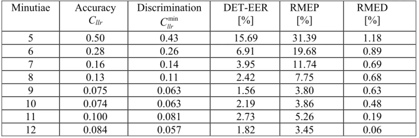
The performance as a function of the number of minutiae is presented using ECE, Tippett and DET plots. The Cllr, Cllrmin, and EER are determined for all minutiae configurations and presented in Table 4.

The ECE plots in Figure 7 show a decreasing trend (solid curves), which corresponds to increased accuracy and discrimination (dashed curves) when increasing the number of minutiae from 5 to 10. The values for the accuracy and discrimination show the same trend and are summarized in Table 4. The sudden increase of these plots and values for the 11-minutiae configurations are related to the comparison algorithm, which changes its method from 11 minutiae onwards.

The Tippett plots in Figure 8 also show coherence of the method with the increasing distance between the curves based on LRs supporting either proposition as the number of minutiae increases. In an ideal system the rates of misleading evidence would be equal to zero, and both curves in the Tippett plots would be maximally separated. The coherence is observed in the Tippett plots when with the increasing number of minutiae there is a decreasing trend in

the rates of misleading evidence and an increase in the separation of the curves. The rate of misleading evidence in favor of Hd (RMED [24, 26]) decreases from 31% for 5-minutiae

configurations to 3.5% for 12-minutiae configurations, while the rate of misleading evidence in favor of Hp (RMEP [24, 26]) decreases from 1.2% for 5-minutiae configurations to 0.06%

for 12-minutiae configurations.

The DET curves in Figure 9 capture the discrimination in a lot more detail, complementing the Tippett plots. Coherent behavior of the LR method used can be observed in the decreasing values of the EER for an increasing number of minutiae. The best performance in terms of EER was achieved for the 9-minutiae configuration dataset (EER = 1.6%). The worst performance of the LR method was observed for the 5-minutiae configuration dataset (EER = 15.7%). Table 4 lists the EER values and apart from the overall decreasing trend shows increases for 10 and 11 minutiae. Not too much meaning can be attached to this because of the overlap and irregular behavior of the DET curves for the highest number of minutiae.

8. DISCUSSION & CONCLUSIONS

The purpose of this article is to introduce coherence as a secondary performance characteristic for LR methods developed for forensic evaluation, and to demonstrate its use with an experimental example. In Section 2 we have split various performance characteristics into primary and secondary ones with examples of factors influencing the primary performance characteristics. We then focused on one performance characteristic in particular – the coherence – by giving an experimental example from the area of forensic fingerprint examination. Coherence has been defined as the property of a given method to perform better when the quality or quantity of information increases, which in our experimental example has been simulated by varying the number of minutiae present in fingermarks from 5 to 12. The performance of the LR method was evaluated using different performance measures (Rates of Misleading Evidence, Cllr and EER) and their corresponding graphical

representations: Tippett, ECE, and DET plots. The LR method used showed coherent behavior: performance increased with the number of minutiae increasing from 5 to 10. It also showed somewhat incoherent behavior and a small decrease in performance when moving from 10 to 11 minutiae.

This incoherent feature of the comparison algorithm’s performance is believed to be caused by a switch of the method it uses when more than 10 minutiae are present. The experimental example therefore reveals the importance of coherence in order to detect points of improvement in computer-assisted LR methods.

REFERENCES

[1] I.W. Evett, Towards a Uniform Framework for Reporting opinions in Forensic Science Casework, Science & Justice, Vol. 38, pp.198-202, 1998

[2] D.V. Lindley, A problem in forensic science, Biometrika 1977, Vol. 64 (2), pp. 207-213 [3] C. Neumann, I. Evett, Quantitative assessment of evidential weight for a fingerprint comparison I. Generalisation to the comparison of a mark with set of ten prints from a suspect, Forensic Sci. Int., 207, pp. 101-105, 2011

[4] A.B. Hepler, Score-based likelihood ratios for handwriting evidence, Forensic Sci. Int., Vol. 219 (1-3), pp. 129-140, 2012

[5] D. Meuwly, Forensic Individualization from Biometric Data, Sci & Jus, Vol. 46 (4), pp. 205 - 13, 2006

[6] N. Egli, Evidence evaluation in fingerprint comparison and automated fingerprint

identification systems – Modelling within finger variability, Forensic Sci. Int. 2007, Vol. 167, pp. 189-195

[7] J. Gonzalez-Rodriguez, J. Fierrez-Aguilar, D. Ramos-Castro and J. Ortega-Garcia, Bayesian analysis of fingerprint, face and signature evidences with automatic biometric systems, Forensic Sci. Int. 2005, Vol. 155, pp. 126-140

[8] G. Zadora, A. Martyna, D. Ramos, C. Aitken. “Statistical Analysis in Forensic Science: Evidential Value of Multivariate Physicochemical Data”. John Wiley and Sons, 2014 [9] J. Gonzalez-Rodriguez, P. Rose, D. Ramos, D. T. Toledano and J. Ortega-Garcia,

"Emulating DNA: Rigorous Quantification of Evidential Weight in Transparent and Testable Forensic Speaker Recognition", IEEE Transactions on Audio, Speech and Language

Processing, Vol. 15, n. 7, pp. 2104-2115, 2007

[10] G.S. Morrison, Measuring the validity and reliability of forensic likelihood-ratio systems, Science & Justice, Vol. 51, pp. 91-98, 2011

[11] European Network of Forensic Science Institutes, Annual Report 2012: http://www.enfsi.eu/news/enfsi-annual-report-2012

[12] R. Gill, FSS Report on Study on Obstacles to Cooperation and Information-sharing among Forensic Science Laboratories and other Relevant Bodies of Different Member States and between these and Counterparts in Third Countries, 2008

http://www.enfsi.eu/sites/default/files/documents/report_project_terrorism_0.pdf [13] ILAC-G19:2002, Guidelines for Forensic Science Laboratories

[14] RvA-T015, 2010, Explanation of NRN-RN ISO/IEC 17025:2005

[15] ISO/IEC 17025:2005, General requirements for the competence of testing and calibration laboratories

[16] D. Ramos, J. Gonzalez-Rodriguez, Reliable support: Measuring calibration of likelihood ratios, Forensic Sci. Int., Vol. 230, pp. 156-169, 2013

[17] D. Ramos, J. Gonzales-Rodriguez, G. Zadora, C. Aitken, Information-Theoretical Assessment of the Performance of Likelihood Ratio Computation Methods, J. Forensic Sci Vol. 58, n. 6, pp. 1503-1518, 2013

[18] N. Brümmer, J. du Preez, Application independent evaluation of speaker detection, Comput Speech Lang, Vol. 20, n. 2-3, pp. 230-75, 2006

[19] I.J. Good, Weight of Evidence: A Brief Survey, Bayesian Statistics 2, pp. 249-270, 1985 [20] D.A. van Leeuwen, N. Brümmer, The distribution of calibrated likelihood-ratios in speaker recognition, in proceedings Interspeech 2013

[21] T. Cover and J. Thomas, Elements of Information Theory 2nd Ed., Wiley & Sons, 2006. [22] J. Quiñonero-Candela, Dataset Shift in Machine Learning Shift in Machine Learning. The MIT Press 2009

[23] C. M. Rodriguez, Introducing a semi-automated method to simulate a large number of forensic fingermarks for research on fingerprint identification, J. Forensic Sci, Vol. 57, n. 2, pp. 334-42, 2012

[24] C. Nemuann et al., Computation of Likelihood Ratios in Fingerprint Identification for Configurations of Three Minutiae, J Forensic Sci, Vol. 51, n. 6, pp. 1255-66, 2006

[25] A. Martin et al., The DET Curve in Assessment of Detection Task Performance, Proc. EuroSpeech (1997) pp. 1895–1898

[26] D. Meuwly, Reconnaissance de Locuteurs en Sciences Forensiques: L’apport d’une Approche Automatique, PhD thesis, 2001

0 200 400 600 800 1000 0.00 0.05 0.10 0.15 0.20

No

rm

al

ize

d

co

un

t

Score

DS Simulated

DS Forensic

0 200 400 600 800 1000 0.00 0.05 0.10 0.15 0.20

No

rm

al

ize

d

co

un

t

Score

DS Simulated

DS Forensic

0.1 0.2 0.5 1 2 5 10 20 40 0.1 0.2 0.5 1 2 5 10 20 40

False Acceptance Probability (in %)

False Rejection Probability (%)

6 minutiae

10 minutiae

−6 −4 −2 0 2 4 6 8 10 0 10 20 30 40 50 60 70 80 90 100

t

Percentage of comparisons with log(LR)>

t

5 minutiae

10 minutiae

−2.5 −2 −1.5 −1 −0.5 0 0.5 1 1.5 2 2.5 0 0.1 0.2 0.3 0.4 0.5 0.6 0.7 0.8

Prior log

(odds)

Empirical cross−entropy

Uncalibrated

Prior log

(odds)

Empirical cross−entropy

Calibrated

−2 −1 0 1 2 0 0.1 0.2 0.3 0.4 0.5 0.6 0.7 0.8 Empirical cross−entropy 5 minutiae −2 −1 0 1 2 0 0.1 0.2 0.3 0.4 0.5 0.6 0.7 0.8 6 minutiae −2 −1 0 1 2 0 0.1 0.2 0.3 0.4 0.5 0.6 0.7 0.8 7 minutiae −2 −1 0 1 2 0 0.1 0.2 0.3 0.4 0.5 0.6 0.7 0.8 8 minutiae LR values After PAV LR=1 always −2 −1 0 1 2 0 0.1 0.2 0.3 0.4 0.5 0.6 0.7 0.8 Empirical cross−entropy 9 minutiae −2 −1 0 1 2 0 0.1 0.2 0.3 0.4 0.5 0.6 0.7 0.8 10 minutiae −2 −1 0 1 2 0 0.1 0.2 0.3 0.4 0.5 0.6 0.7 0.8 11 minutiae 0 0.1 0.2 0.3 0.4 0.5 0.6 0.7 0.8 12 minutiae Figure7

−4 −2 0 2 4 6 8 0 10 20 30 40 50 60 70 80 90 100 t

Percentage of comparisons with log(LR)>

t 5 minutiae 6 minutiae 7 minutiae 8 minutiae 9 minutiae 10 minutiae 11 minutiae 12 minutiae Figure8

0.1 0.2 0.5 1 2 5 10 20 40 0.1 0.2 0.5 1 2 5 10 20 40

False Acceptance Probability (in %)

False Rejecti

on Probability (in %)

FIGURE CAPTIONS

Figure 1

Forensic (left) vs. simulated (right) fingermark.

Figure 2

Normalized score distribution for 5-minutiae configurations of forensic versus simulated datasets (lowest degree of similarity).

Figure 3

Normalized score distribution for 6-minutiae configurations of forensic versus simulated datasets (highest degree of similarity).

Figure 4

DET curves showing the performance of the same LR method with different quantities of information. The dashed curve shows worse discrimination in the LRs of comparisons for 6-minutiae configurations, while the solid line shows better discrimination in the LRs of comparisons for 10-minutiae configurations. The equal error rates are given by the

intersection of the curves with the diagonal of the plot, and are 6.9% and 2.2%, respectively.

Figure 5

Tippett plots showing the performance of the same LR method with different quantities of information. Dashed lines show less evidential information captured in the LRs of

comparisons for 5-minutiae configurations, while solid lines show more evidential information captured in the LRs of comparisons for 10-minutiae configurations.

Figure 6

ECE plots for the same LR method (same set of LR values) before and after calibration (leave one out cross-validation used for calibration). On the left-hand-side the solid curve represents uncalibrated LRs, and the dashed curve gives the ECE after PAV. The LRs on the right-hand-side are calibrated using the PAV transform resulting from the data used for the left ECE plot. The dramatic lack of calibration is visible in the left plot by the fact that above prior-log(odds) = 0.5 the ECE exceeds that of the reference method which always gives

LR = 1). For that range of prior odds the uncalibrated method performs worse than a method that always returns the “I don’t know” answer (i.e., always yielding LR = 1).

Figure 7

ECE plots for LRs generated for forensic marks with 5 to12-minutiae configurations. Note the different scaling of the y-axis in the upper and lower row of plots.

Figure 8

Tippett plots for LRs generated for forensic marks with 5 to12-minutiae configurations.

Figure 9

TABLES

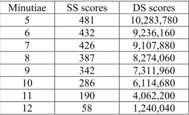
Table 1: Forensic dataset sizes, for SS and DS scores. Note that the number of SS scores is the same as the number of clusters for a given number of minutiae.

Minutiae SS scores DS scores

5 481 10,283,780 6 432 9,236,160 7 426 9,107,880 8 387 8,274,060 9 342 7,311,960 10 286 6,114,680 11 190 4,062,200 12 58 1,240,040

Table 2: Simulated dataset sizes for SS and DS scores.

Minutiae SS scores DS scores

5 16,653 33,306,000 6 25,058 50,116,000 7 24,876 49,752,000 8 25,015 50,030,000 9 25,036 50,072,000 10 24,994 49,988,000 11 24,658 49,316,000 12 24,443 48,886,000

Table 3: KLsym divergence of the DS comparison scores (simulated and forensic dataset).

Minutiae KLsym 5 0.034 6 0.007 7 0.011 8 0.019 9 0.013 10 0.010 11 0.014 12 0.011 Tables_1_4

Table 4: Increase in performance of the LR method when introducing additional minutiae. Minutiae Accuracy Cllr Discrimination min llr C DET-EER [%] RMEP [%] RMED [%] 5 0.50 0.43 15.69 31.39 1.18 6 0.28 0.26 6.91 19.68 0.89 7 0.16 0.14 3.95 11.74 0.69 8 0.13 0.11 2.42 7.75 0.68 9 0.075 0.063 1.56 3.80 0.63 10 0.074 0.063 2.19 3.86 0.48 11 0.100 0.081 2.73 5.26 0.19 12 0.084 0.057 1.82 3.45 0.06

ACKNOWLEDGEMENTS

This research was conducted in the scope of the BBfor2 – European Commission Marie Curie Initial Training Network (FP7-PEOPLE-ITN-2008 under Grant Agreement 238803) at the Netherlands Forensic Institute, and in collaboration with the ATVS Biometric Recognition Group at the Universidad Autonoma de Madrid and the National Police Services Agency of the Netherlands.