Pervasive Data Analytics for Sustainable Energy Systems

POUR L'OBTENTION DU GRADE DE DOCTEUR ÈS SCIENCES

acceptée sur proposition du jury: Prof. B. Faltings, président du jury Prof. K. Aberer, directeur de thèse

Prof. T. B. Pedersen, rapporteur Dr M. Sinn, rapporteur Prof. J.-Y. Le Boudec, rapporteur

Pervasive Data Analytics for Sustainable Energy Systems

THÈSE N

_{6556 (2015)}

ÉCOLE POLYTECHNIQUE FÉDÉRALE DE LAUSANNE

À LA FACULTÉ INFORMATIQUE ET COMMUNICATIONS LABORATOIRE DE SYSTÈMES D'INFORMATION RÉPARTIS PROGRAMME DOCTORAL EN INFORMATIQUE ET COMMUNICATIONS

Suisse 2015

PAR

Pervasive Data Analytics for Sustainable Energy Systems

Tri Kurniawan WIJAYA

Abstract

With an ever growing population, global energy demand is predicted to keep increasing. Fur-thermore, the integration of renewable energy sources into the electricity grid (to reduce carbon emission and humanity’s dependency on fossil fuels), complicates efforts to balance supply and demand, since their generation is intermittent and unpredictable. Traditionally, it has always been the supply side that has adapted to follow energy demand, however, in order to have a sustainable energy system for the future, the demand side will have to be better managed to match the available energy supply.

In the first part of this thesis, we focus on understanding customers’ energy consumption be-havior (demand analytics). While previously, information about customer’s energy consumption could be obtained only with coarse granularity (e.g., monthly or bimonthly), nowadays, using advanced metering infrastructure (or smart meters), utility companies are able to retrieve it in near real-time. By leveraging smart meter data, we then develop a versatile customer segmen-tation framework, track cluster changes over time, and identify key characteristics that define a cluster.

Additionally, although household-level consumption is hard to predict, it can be used to improve aggregate-level forecasting by first segmenting the households into several clusters, fore-casting the energy consumption of each cluster, and then aggregating those forecasts. The improvements provided by this strategy depend not only on the number of clusters, but also on the size of the customer base. Furthermore, we develop an approach to model the uncertainty of future demand. In contrast to previous work that used computationally expensive methods, such as simulation, bootstrapping, or ensemble, we construct prediction intervals directly using the time-varying conditional mean and variance of future demand.

While analytics on customer energy data are indeed essential to understanding customer behavior, they could also lead to breaches of privacy, with all the attendant risks. The first part of this thesis closes by exploring symbolic representations of smart meter data which still allow learning algorithms to be performed on top of them, thus providing a trade-off between accurate analytics and the protection of customer privacy.

In the second part of this thesis, we focus on mechanisms for incentivizing changes in cus-tomers’ energy usage in order to maintain (electricity) grid stability, i.e., Demand Response (DR). We complement previous work in this area (which typically targeted large, industrial cus-tomers) by studying the application of DR to residential customers. We first study the influence of DR baselines, i.e., estimates of what customers would have consumed in the absence of a DR event. While the literature to date has focused on baseline accuracy and bias, we go beyond these concepts by explaining how a baseline affects customer participation in a DR event, and how it affects both the customer and company profit. We then discuss a strategy for matching the demand side with the supply side by using a multiunit auction performed by intelligent agents

ii Abstract on behalf of customers. The thesis closes by eliciting behavioral incentives from the crowd of customers for promoting and maintaining customer engagement in DR programs.

Keywords: smart grid, data analytics, customer segmentation, smart meter, load forecasting, privacy, demand response, sustainability, dynamic pricing, multi-agent system, human behavior, crowdsourcing

R´

esum´

e

La croissance continuelle d´emographique entraˆınera une augmentation de la demande mondiale ´

energ´etique. De plus, l’int´egration de sources d’´energie renouvelable dans le r´eseau ´electrique (pour r´eduire les ´emissions de carbone et la d´ependance de l’humanit´e aux ´energies fossiles) rend difficiles les efforts pour ´equilibrer l’offre et la demande, du fait de la nature intermittente et impr´evisible de leur g´en´eration. Traditionnellement, l’offre s’adaptait `a la demande ´energ´etique. Cependant, dans le cadre d’un future syst`eme ´energ´etique durable, la demande devra ˆetre mieux g´er´ee pour ˆetre assortie `a l’offre ´energ´etique disponible.

Dans la premi`ere partie de cette th`ese nous nous concentrons sur la compr´ehension du com-portement ´energ´etiques des utilisateurs (analyse de la demande). Alors que des information sur la consommation ´energ´etique des clients ne pouvaient ˆetre obtenues qu’`a une granularit´e grossi`ere (e.g., mensuellement ou bi-mensuellement), de nous jours, grˆace aux infrastructures de comptage avanc´e (ou compteurs intelligents ou smart meters), les compagnies d’´electricit´e peu-vent les obtenir en temps r´eel. En tirant parti des donn´ees de smart meters, nous developpons un framework versatile pour segmenter les clients, suivons les changements des clusters `a travers le temps et identifions les caract´eristiques cl´es qui d´efinissent un cluster.

Additionnellement, bien que la consommation au niveau r´esidentiel est difficilement pr´evisible, il peut ˆetre utilis´e pour am´eliorer les pr´evisions au niveau agr´eg´e en segmentant d’abord les m´enages en plusiers clusters, puis en pr´edisant la consommation d’´energie de chaque cluster et enfin en agr´egeant ces pr´evisions. Les am´eliorations fournies par cette strat´egie d´ependent non seulement du nombre de clusters, mais aussi de la taille de la client`ele desservie. En outre, nous developpons une approche pour mod´eliser l’incertitude de la demande future. En contraste avec les travaux ant´erieurs qui utilisaient des m´ethodes de calculs coteuses, comme la simulation, le bootstrapping ou l’ensemble, nous construisons des intervalles de pr´ediction utilisant directement la moyenne conditionnelle et la variance, variables dans le temps, de la demande future.

Bien que l’analyse des donn´ees de consommation d’´energie des clients soient essentielles pour comprendre les comportements des clients, elle peut aussi violer leur vie priv´ee, avec tous les risques y attenant. La premi`ere partie de cette th`ese se conclut par l’exploration de repr´esentations symboliques des donn´ees de smart meter qui permettent aux algorithmes d’apprentissages de les utiliser similairement. Celles-ci pr´esentent donc un compromis entre analyse pr´ecise et la protection de la vie priv´ee des clients.

Dans la seconde partie de cette th`ese, nous nous concentrons sur des m´ecanismes pour inciter des changements dans l’utilisation d’´energie par les clients dans le but de maintenair la stabilit´e du r´eseau ´electrique, i.e. dans le cadre de la r´eaction `a la demande (Demand Response ou DR). Nous compl´etons le travail ant´erieur dans ce domaine (qui ciblait g´en´eralement de grands clients industriels) en ´etudiant l’application de DR aux clients r´esidentiels. Nous ´etudions tout d’abord l’influence de donn´ees de r´ef´erence de DR, i.e. des estimations de la consommation des clients en l’absence d’´ev´enement de DR. Alors que la litt´erature `a ce jour s’est concentr´ee sur la pr´ecision et

iv R´esum´e le biais de r´ef´erence, nous avous avons d´epass´e ces concepts en expliquant comment une valeur de r´ef´erence affecte la participation du client `a un ´ev´enement de DR et comment ceci impacte tant le client, que le profit de la compagnie. Nous poursuivons par la pr´esentation d’une strat´egie pour accorder la demande `a l’offre en utilisant une syst`eme d’ench`eres `a multiples unit´es accomplies par des agents intelligents au nom des clients. Cette th`ese se conclut par l’obtention de mesures incitatives comportementales issues de la client`ele pour promouvoir et maintenir la participation des clients dans les programmes de DR.

Mots-cl´es : smart grid, analyse de donn´ees, segmentation des clients, smart meter, pr´evisions de charge, vie priv´ee, demand response, durabilit´e, tarification dynamique, syst`eme multi-agents, comportement humain, crowdsourcing

Acknowledgements

First and foremost, I would like to thank my advisor, Karl. This thesis would not exist without him. In the admission interview, I told him: “but, I do not have the background (e.g., P2P) that your lab has.” He replied, “It’s ok. That, you can learn. The more important things are your attitude and your potential.” Since then, I knew that I will try my best, day and night, to not let him down. I am very grateful that he always believes in me. He gives me enough freedom to take initiative on my research. I like that very much. He has vast experiences and is very good at what he is doing. He could look into the paper that I have written, spotted a flaw, told me about it, and (after fixing it) it eventually became one of the paper strengths. Sometimes it took me days before I could digest what Karl said. He is able to see far away things that did not even cross my mind. And I think that it’s cool! Lately, do not want to miss his wisdom, I asked his permission to record our meetings. He agreed. Then, of course, I needed to play it several times before I understand them ¨^In short, I cannot ask for a better advisor.

I would like to thank my thesis committee: Prof. Faltings, Prof. Le Boudec, Prof. Pedersen, and Mathieu. I can’t thank them enough for their precious time and availability. Especially to Prof. Pedersen and Mathieu who had to travel for attending my defense. They are leaders in their fields and have a lot of experiences as well. Every single discussion with them is sharp and constructive.

I would like to thank Matteo. It is hard to imagine completing this thesis without him. Working with him has been a privilege. He is a genuinely nice person and great colleague. Sharing similar academic background and interest, our collaboration simply ‘click.’ Everything moves very fast. We also challenge each other ideas at times, but in positive and constructive ways. Our collaboration is not an addition, it is a multiplication.

I would like to thank the Wattalyst consortium. To Thanasis, Dipanjan, and Zhixian that helped me to ‘take off’ in my first year. To Deva and Tanuja who hosted me in their Smarter Energy group in IBM Research India, summer 2013. The collaboration with them has been very fruitful and is the heart of Chapter 3. And to other partners: Mikael, Arne, and Jan from LTU, Achim from RWTH Aachen, George S., George T., and Marilena from AUEB, I˜niaki and Mikel from Tecnalia, and Pau, Carlos and Maria from Sampol, our face to face meetings have always been insightful and full of joy. Wattalyst has ‘raised’ me. From knowing almost nothing, I grew and learned from every discussion we made.

I would like to thank my colleagues and friends during my internship at IBM Research Ireland, early 2014. Especially to Mathieu (again ¨^) and Bei for their unlimited patience. They often have to explain some basic concepts to me (because somehow I have never heard of them) until it became crystal clear to me. All good things in Chapter 5 is because of them. To Hussein, coming from the same institution, EPFL, we only met each other at IBM Research Ireland (both of us were interns at that time). I learned a lot from him, especially the kind of basic/fundamental (machine learning related) questions that you always wanted to know but were afraid to ask.

vi Acknowledgements He explained them effortlessly. To Olivier who introduced me to the CER dataset, in summer 2012. The dataset soon became my favorite. In addition to Chapter 3, 4, and 7 in this thesis, the dataset has also contributed to several other publications that I co-authored.

I would like to thank Kate Larson. She was very instrumental in introducing me to multiagent system. It is hard to imagine completing Chapter 8 without her.

I would like to thank Julien. We have several collaborations, where one of them resulted in Chapter 6. A very talented friend. Being one of the two Swiss in our lab (surprisingly small number, btw), I abused him with lots of questions about Swiss.

I would like to thank Samuel, a smart student whose work paved the way for Chapter 4. I would like to thank Ulysse Rosselet for introducing the open innovation crowdsourcing platform, Atizo. He also helped me to set up the crowdsourcing experiment in Chapter 9.

I would like to thank Hˆong- ˆAn for helping me with the French abstract. Together with Christoph, their knowledge about SBB and wine collection amazes me.

I would like to thank Zico Kolter. We have never met, but Chapter 1 is inspired by his CMU lectureComputational Methods for the Smart Grid.

I would like to thank Darren for proofreading part of this thesis.

I would like to thank Chantal for her support in administrative tasks. I asked her a lot of questions, from formal to informal, from regulations to social norm, about our lab, EPFL, Lausanne, and Switzerland. Working at the EPFL without her would be very hard.

I would like to thank all my friends. To Waheed who guided me to EPFL. Being friends since we were in Dresden, I practically follow his path to go to EPFL. To Myriam, Aleksandra, and Khoa, I cannot ask for better flatmates. I am very lucky to have them. To Fauziah, mbak Henny, mbak Rini, Ihan, Yolanda, and Aufar. Every moment I spent with them is simply a joy. Not only because I can freely speak Indonesian, but also because I can act and eat Indonesian. To my office mate, Alexandra. I learned a lot from her. About academics, humanity, and ... disaster (yep, this is what she cares about now ¨^). To Mehdi and Pamela, I remember as if it was yesterday, we sit together at the top of the BC building, together with Alexandra, enjoying the warm sunny weather and eating together during the MICS summer school 2011, prior to joining EPFL. To Hoyoung, Zoltan, Sofiane, Rammohan, Surender, Saket, Hung, Michele, Tian, Jean-Eudes, Jean-Paul, Rameez, Hamza, Hao, Martin, Berker, Alevtina, Sarvenaz, Tomasso, Tam, Amit, Iuliia, Burak, Nataliya, and Imen. To Amitabh & Mohita, Jiaqing, Mihai, Florin, Lauren, and Jasmina. To all friends in EDIC. Without them, life in EPFL and Switzerland would only be half as good.

To Andrea, for her constant love and support that are much bigger than I can imagine. I am deeply thankful and grateful for her presence in my life. Stars have been much brighter since then. Also to her family for their encouragement. It’s always fun to be near them.

And the last but not the least, to my family, who always believe in me. No words can express my gratitude towards them. Especially to my mom, my sister, and aunt Lily who never stop supporting me. I am very lucky to have them. They put their faith in me, letting me go more than ten thousand kilometers away to chase my dream.

Contents

1.1 Developing Sustainable Energy Systems . . . 1

1.1.1 Today’s Energy Challenges . . . 1

1.1.2 The Smart Grid . . . 3

1.1.3 Demand-Side Participation . . . 5

1.1.4 The Role of Computer Science . . . 8

1.2 Thesis Scope and Contributions . . . 10

2 State of the Art 13 2.1 Demand Analytics . . . 13

2.1.1 Customer Segmentation . . . 13

2.1.2 Load Forecasting . . . 15

2.2 Demand Response . . . 18

2.2.1 Energy Consumption Scheduling . . . 19

2.2.2 Storage Devices . . . 20

2.2.3 Cooperatives . . . 21

2.2.4 Electric Vehicles . . . 23

I

Demand Analytics

25

3.2 Context-Based Customer Segmentation . . . 29

3.2.1 Design Principles . . . 29

viii Contents

3.2.2 The Framework . . . 29

3.3 Clustering Consistency . . . 35

3.3.1 Individual to Cluster Consistency . . . 35

3.3.2 Distance Rank . . . 36

3.3.3 Cluster Configuration Consistency . . . 36

3.4 Knowledge Extraction from Survey Data . . . 36

3.4.1 Discriminative Index . . . 37

3.4.2 Dealing with Ordinal and Quantitative Data . . . 37

3.4.3 An Alternative to Discriminative Index . . . 38

3.5 Experimental Evaluations . . . 39

3.5.1 Dataset . . . 39

3.5.2 Customer Segmentation . . . 39

3.5.3 Clustering Consistency . . . 41

3.5.4 Knowledge Extraction from Survey Data . . . 43

3.6 Summary and Discussion . . . 47

4 Forecasting Residential Demand 49 4.1 Introduction . . . 49

4.2 Dataset and Evaluation Metrics . . . 50

4.2.1 Dataset . . . 50 4.2.2 Evaluation Metrics . . . 51 4.3 Forecasting Models . . . 52 4.3.1 Features . . . 52 4.3.2 Learning Algorithms . . . 52 4.4 Individual Forecasting . . . 54 4.5 Aggregate Forecasting . . . 56 4.5.1 Clustering Algorithms . . . 57

4.5.2 The Impact of the Size of the Customer Base . . . 58

4.6 Summary and Discussion . . . 60

5 Modeling Uncertainty of Future Demand 63 5.1 Introduction . . . 63

5.2 Modeling Uncertainty . . . 65

5.2.1 The GAM2Algorithm . . . 65

5.2.2 Evaluation Metrics . . . 67 5.3 Online Learning . . . 68 5.4 Experimental Results . . . 68 5.4.1 Dataset . . . 69 5.4.2 Forecasting Uncertainty . . . 69 5.4.3 Online Learning . . . 70

5.5 Summary and Discussion . . . 73

6 Reducing Data Size and Privacy Risk 75 6.1 Introduction . . . 75 6.2 Symbolic Representation . . . 76 6.2.1 Vertical Segmentation . . . 76 6.2.2 Horizontal Segmentation . . . 77 6.2.3 Compression Ratio . . . 79 6.3 Experiments . . . 79

Contents ix

6.3.1 Classification . . . 81

6.3.2 Forecasting . . . 82

6.4 Summary and Discussion . . . 85

II Demand Response

87

7.2 Demand Response Baselines . . . 90

7.2.1 HighXofY . . . 91

7.2.2 LowXofY . . . 92

7.2.3 MidXofY . . . 92

7.2.4 Exponential Moving Average . . . 92

7.2.5 Regression . . . 93

7.3 Residential Demand Response . . . 94

7.3.1 DR Signal . . . 94

7.3.2 DR Event . . . 94

7.3.3 Cost and Profit Functions . . . 95

7.3.4 Customer Model . . . 97

7.4 Accuracy and Bias . . . 97

7.4.1 Setup . . . 97

7.4.2 Analysis . . . 98

7.5 Net Benefit Analysis . . . 99

7.5.1 Setup . . . 99

7.5.2 Customers Profit . . . 99

7.5.3 Company’s Profit . . . 102

7.6 Summary and Discussion . . . 103

8 Matching Demand with Supply 105 8.1 Introduction . . . 105

8.2 Preliminaries . . . 106

8.2.1 Load Modeling . . . 106

8.2.2 Multiunit Auction . . . 107

8.3 PAR-Cut . . . 108

8.4 Multiunit Auction for Load Distribution . . . 109

8.4.1 Initial Condition . . . 109

8.4.2 Minimal Load Guarantee . . . 110

8.4.3 Initial Pricing . . . 110

8.4.4 The Auction: Matching Demand Against Supply . . . 110

8.4.5 Customer’s Load Shifting . . . 112

8.4.6 Customer’s Utility . . . 112

8.5 Experiments . . . 112

8.5.1 Experiment Setup . . . 112

8.5.2 System Cost . . . 113

8.5.3 Customers’ Utility . . . 113

8.5.4 Customers’ Additional Benefit . . . 114

8.5.5 Company’s Additional Benefit . . . 115

x Contents

9 Crowdsourcing Behavioral Incentives 117

9.1 Introduction . . . 117 9.2 Behavioral Framework . . . 118 9.2.1 Motivation . . . 119 9.2.2 Ability . . . 119 9.2.3 Triggers . . . 119 9.3 Crowdsourcing Experiment . . . 120 9.3.1 Crowdsourcing . . . 120 9.3.2 The Experiment . . . 120 9.4 Analysis of Results . . . 121 9.4.1 Submission Statistics . . . 121 9.4.2 Motivation . . . 121 9.4.3 Simplicity . . . 123 9.4.4 Trigger . . . 124

9.5 Crafting New Solutions . . . 125

9.6 Summary and Discussion . . . 127

IIIConclusion

129

10.2 What’s Next? . . . 133

Bibliography 135

List of Figures

1.1 World annual energy consumption in petawatt-hours, i.e., 1015 Watt-hours [Roser,

2014b]. We converted the original figure, in Exajoules, to Watt-hours so as to be consistent with the rest of the thesis. This figure does not show the share of renewable energy sources such as wind and solar, which is approximately less than half that of hydro power’s: hydro power constitutes around 2.4% of the world energy mix; other renewable energy sources currently amount to only 1.1% [International Energy Agency,2014]. . . 1

1.2 (a) World population estimate [Kremer, 1993, Roser, 2014c, United Nations, 2014,

U.S. Census Bureau,2014]; (b) World annual energy consumption per capita—computed by dividing the total world energy consumption in Figure 1.1 by the world population estimate. . . 2

1.3 (a) World CO2 emission [Roser, 2014a]; (b) Global atmospheric concentrations of

carbon dioxide over time [U.S. Environmental Protection Agency,2014]. . . 2

1.4 A simplified illustration of how key grid components relate to suppliers (and/or utility companies) and customers. EMS, energy management systems. DG, distributed generation. . . 4

1.5 A sample (3 weeks) of wind power production and electricity demand in western Denmark [Kok, 2013]. The top figure is the situation in 2008, where 20% of total demand was covered by wind power. The bottom figure is the expected situation in 2025 where wind power is projected to cover 50% of demand. Note that, the production curve rarely matches the demand. . . 5

1.6 An illustration of supply and demand curves during the California energy crisis in summer 2000 [Hirst and Kirby,2001]. P, price. Q, demand. The market clears at 29 GW for $550/MWh. If consumers are even modestly sensitive to prices, the market could clear at 27.5 GW for $250/MWh. The dashed line is a demand curve with a price elasticity of about 0.03. . . 7

2.1 An illustration of the herding effect [Wijaya et al., 2013d]. The cost depends on the squared load. The peak hour is initially at time slott1 (which costs 8 per unit).

Afterwards, A and B shift their consumption to timet2(since it previously costs only

0 per unit). Rather than flattening the peak (and reducing cost), it causes a peak-shifting and makest2 the new peak. The peak load and total cost can be reduced if

only A or B (but not both) makes the shift. . . 20

xii List of Figures 2.2 An example of a service curve [Le Boudec and Tomozei,2011]. Intuitively, it allows

a utility company to serve no power to a customer for at most 30 minutes in a day (or serve (1−1

x)zmax watt forx·30 minutes, wherex∈[1,48]), and guaranteezmax

watt for the rest of the day. . . 20 2.3 nPlug prototype [Ganu et al.,2013]. . . 21 2.4 An illustration of the energy market structure with the existence of smart load

bal-ancing group [Vasirani and Ossowski, 2013]. From the market point of view, the aggregator is a single buyer (similar to other retailers). . . 23

3.1 Smart metering projects map around the world [Harrison, 2013]. Retrieved: 7 Jan-uary 2015. . . 28 3.2 Architecture diagram of the framework. . . 30 3.3 Feature f1 is discriminative positive for clusterc1, whereasf2 is discriminative

neg-ative forc1. While entropy measure is able to recognize only discriminative positive

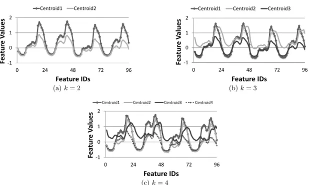
features, our discriminative index is able to recognize both, discriminative positive and negative features. . . 38 3.4 Centroids of clusters using January data, and hourly temporal aggregation. For the

features, we use normalized mean of weekday (ID 1-24), normalized mean of weekend (ID 25-48), normalized median of weekday (ID 49-72), and normalized median of weekend (ID 73-96) consumption. We use kMeans algorithm withk= 2,k= 3, and

k= 4. . . 40 3.5 Customer segmentation on consumption trends (a)-(c), absolute consumption

(d)-(f), and consumption variability (g)-(i), in different contexts: January, July, and all months. For trends, we used the same features as in Figure 3.4. Feature ID 1-24 and 49-72 are weekdays consumption, whereas 25-48 and 73-96 are weekend consumption. We use mean (ID 1-48) and median (ID 49-96) for absolute, and standard deviation and IQR for variability. . . 42 3.6 (a) cluster configuration consistency over time (monthly), consumption profile using

(b) January 2010 data, (c) July 2010 data, and (d) cluster configuration consistency over different temporal aggregations. . . 43 3.7 Cumulative distribution of (a) floor area, and (b) the year customers’ houses was

built. Customers are clustered by their absolute consumption: low, medium, and high. 45 3.8 Fraction of households which own games consoles for different family types. . . 46

4.1 MLP model evaluation (using NRMSE) using different number of hidden layers and learning rates α on randomly chosen 25 households. The lower the better. In the end, we use one hidden layer andα= 0.1. . . 53 4.2 SVR model evaluation for individual forecasting on the randomly chosen 25

house-holds: (a) average NRMSE on the validation set given differentCandγ, (b) standard deviation on the average, (c) average running time. The lower the better. In the end, we choose C = 100 and γ = 0.01. While there are some other settings which yield better NRMSE, they typically require considerably longer running time. . . 53 4.3 SVR model evaluation (measured by average NRMSE) for aggregate forecasting. The

lower the better. . . 54 4.4 A sample of hourly energy consumption from the CER dataset, from Monday,

2009-09-07 to Sunday, 2009-09-13. . . 56 4.5 The NRMSE of LR and SVR for 1 hour ahead forecasting (the lower the better).

List of Figures xiii 4.6 The NRMSE, the NMAE and the MAPE for a different number of clustersk (the

lower the better). Total number of customers, N = 3639. The best accuracy is obtained when 1< k <3639, which shows the effectiveness of CBAF. . . 59 4.7 Percentage improvement in the NRMSE of the CBAF strategy (compared to the

traditional aggregate forecast,k= 1) of 500, 1,000, 2,000, and 3,639 customers over a different number of clusters and clustering methods (the higher the better). The larger the customer set, the higher the improvement gained by CBAF. . . 60

5.1 Hourly electricity demand in France; (a) the complete view of the dataset (from January 2003 to December 2012), and (b) the first week of the dataset. . . 69 5.2 Visualization of some transfer functions from the model in Eq. 5.11. It illustrates an

additional benefit of using GAM, i.e., its transfer functions provide insights about the relationship between explanatory and target variables: (a) represents the typical hourly load curve on Monday, (b) the yearly seasonality of electricity demand, where the winter demand is typically lower than that of summer, (c) the joint effect of temperature and hour of the day. The dip aroundTimeOfYear= 0.6 in (b) shows the effect of school summer holiday. Note that, the function outputs above are of small magnitude since the model considers the logarithmic of the demand. . . 71 5.3 Normal Q-Q plot of (a) the empirical residualsz_bt, (b) the rescaled residualsbt. . . . 72 5.4 Prediction intervals of the first week (Sunday–Saturday) of the test set #1 (see

Ta-ble 5.1). The black line is the actual demand, the red line is the forecasted expected demand, and the green lines are the prediction intervals (from bottom to top: one-sided prediction intervals for 1 to 99 percentiles). . . 72 5.5 The mean percentage width (MPW) and the coverage absolute error (CAE) of the

estimated (a) one- and (b) two sided prediction intervals, averaged over the two test periods. . . 73 5.6 The forecasting error (MAPE) over time for the two models, i.e., with and without

online learning. The online learning mechanism succeeds to keep the forecasting error low over time. . . 73 5.7 Empirical coverage (a) without and (b) with adaptive interval construction over time.

The solid lines represent the two-sided coverages for the (from top to bottom) 90, 80, ..., 20, and 10 percentiles. The numbers on the right hand side show the empirical coverages at the end of the test period. The dotted lines are the binomial (95%) confidence interval for each percentile, which serve as a guide on approximate ranges of acceptable coverages. . . 74

6.1 Construction of the variable length of symbols by recursive division of the real values range. . . 77 6.2 Distribution of Energy levels with 1 second sampling rate in the REDD dataset follows

a log-normal distribution. . . 78 6.3 Without normalization A and B (C and D) are more similar, but with normalization

A and C (resp. B and D) would be put together. . . 79 6.4 Statistics on energy consumption of house 1 in REDD dataset (86400 seconds = 1

day). . . 80 6.5 Evaluation of a Naive Bayes classifier over symbolic and raw data. . . 81 6.6 Evaluation of a Random Forest classifier over symbolic and raw data. . . 82 6.7 Evaluation of a Random Forest classifier over symbolic (using a single lookup table)

xiv List of Figures 6.8 MAE of symbolic forecasting using Naive Bayes. Forecasting performance using raw

value is shown for comparison. House 5 is skipped because there is not enough data. 85 6.9 MAE of symbolic forecasting using Random Forest. Forecasting performance using

raw value is shown for comparison. House 5 is skipped because there is not enough

data. . . 85

7.1 An illustration of the true baseline, predicted baseline, and actual load where a DR event occurs from 17:00 to 20:00 to curtail the evening peak. . . 95

7.2 Mean Average Error (MAE) and bias of different baselines in kWh. Average hourly load over all customers is 0.97 kWh. . . 98

7.3 Received incentive and additional profit in the naive customer model with variousγ (x-axis). Both are calculated as the sum of customers over all 52 DR events. . . 100

7.4 Received incentive and additional profit in the rational customer model with various γ (x-axis). Both are calculated as the sum of all customers over all 52 DR events. . 100

7.5 The evolution of γ, received incentive, and additional profit of adaptive customer model withγ0_{= 0.2 andα= 0.1 (defined in Section 7.3.3). Received incentives and} additional profit shown are the sum over all customers and 52 DR events. . . 101

7.6 Company’s profit under different customer models and variousα. . . 102

8.1 Overall system cost decrease as the cut percentage getting larger. Simulation using 10000 households loads. . . 113

8.2 Customers’ utility based on shift percentage measurement (defined in Section 8.4.6) grouped by their valuation (US distribution). . . 113

8.3 Customers’ utility based on shift percentage measurement (defined in Section 8.4.6) grouped by their valuation (uniform distribution). . . 114

8.4 Customers’ utility based on the total cost paid (defined in Section 8.4.6) grouped by their valuation (US distribution). . . 114

8.5 Customers’ utility based on the total cost paid (defined in Section 8.4.6) grouped by their valuation (uniform distribution). . . 114

8.6 Customers’ cost saving percentage using the auction and PAR cut compare to the current system. Valuation used: US distribution. . . 115

8.7 Company addition revenue from the auction. . . 115

9.1 Fogg’s Behavior Model (source: Fogg, 2009) . . . 118

9.2 Home page of our crowdsourcing challenge . . . 121

9.3 Number of submissions per participant . . . 122

9.4 Number of submissions over time . . . 122

9.5 A word cloud generated from the submissions . . . 123

9.6 Motivation . . . 124

9.7 Simplicity . . . 125

List of Tables

1.1 A summary of DR program benefits and costs [Albadi and El-Saadany,2008]. . . 8

3.1 Customer characteristics based on their absolute consumption. A minus (-) sign denotes discriminative negative. . . 43 3.2 Customer characteristics based on their consumption variability. A minus (-) sign

denotes discriminative negative. . . 44 3.3 Discriminative appliances’ ownership for different clusters based on their absolute

consumption. We show only for DI ≥ 0.60 and support ≥ 0.40. A minus (-) sign denotes discriminative negative. . . 46 3.4 Discriminative appliances’ ownership for different clusters based on their consumption

variability. We show only for DI≥0.60 and support≥0.40. A minus (-) sign denotes discriminative negative. . . 46

4.1 Average NRMSE and NMAE (with its 95% confidence interval) of LR, MLP,SVRfor 1 hour ahead load forecasting at the level of the individual customer. Benchmark (bm) isst−1. The numbers in parentheses show the improvements compared to the

benchmark. Root transformation (st1/p, withp >1) can be used to improve NMAE. 55

4.2 Average NRMSE and NMAE (with its 95% confidence interval) of LR,MLP, SVRfor 24 hour ahead load forecasting at the level of the individual customer. Benchmark (bm) isst−24. The numbers in parentheses show the improvements compared to the

benchmark. Root transformation (st1/p, withp >1) can be used to improve NMAE. 55

4.3 Average NRMSE and NMAE (with its 95% confidence interval) of Seasonal ARIMA (SARIMA) for 1 hour and 24 hour ahead individual load forecasting. Benchmark (bm) isst−1 for 1 hour ahead forecasting andst−24for 24 hour ahead forecasting. We use

the pth root transformation (st1/p), with p = 2. The numbers in the parentheses

show the improvements compared to the benchmarks. . . 55

5.1 Our out-of-sample, non-overlapping, rolling window test period. . . 69

6.1 F-measure for each method with 1 hour and 15 minutes aggregation, with 2 to 16 symbols, using Random Forest (RF), J48 decision tree, Na¨ıve Bayes (NB), and Lo-gistic Regression. + means that the encoding use a single lookup table for all houses.

. . . 84

7.1 Summary of the baseline methods. . . 93 7.2 Detailed characteristics of ISONE, Low4of5, Mid4of6, Reg2, and NYISO (ordered by

MAE). . . 99

Introduction

1

1.1

Developing Sustainable Energy Systems

1.1.1

Today’s Energy Challenges

Sustainable development is defined by the United Nations as development that meets the needs of the present without compromising the ability of future generations to meet their own needs [World Commission on Environment and Development,1987]. World energy consumption, however, has increased rapidly since the industrial revolution in the 1800s (see Figure 1.1) Its cause is not only the increasing world population, but also the increasing energy consumption per capita (Figure 1.2). Unfortunately, more than 80% of humanity’s energy consumption is made possible

0 25 50 75 100 125 1800 1850 1900 1950 2000 PW h Year Nuclear Hydro Natural Gas Oil Coal Biofuels

Figure 1.1: World annual energy consumption in petawatt-hours, i.e., 1015 Watt-hours [Roser,2014b].

We converted the original figure, in Exajoules, to Watt-hours so as to be consistent with the rest of the thesis. This figure does not show the share of renewable energy sources such as wind and solar, which is approximately less than half that of hydro power’s: hydro power constitutes around 2.4% of the

world energy mix; other renewable energy sources currently amount to only 1.1% [International Energy

Agency,2014].

2 Introduction 0 2 4 6 8 10 1800 1850 1900 1950 2000 2050 bi llio ns Year U.N. projection U.S. Census Bureau Kremer's estimates (a) 0 5 10 15 20 1800 1850 1900 1950 2000 MWh Year Nuclear Hydro Natural Gas Oil Coal Biofuels (b)

Figure 1.2: (a) World population estimate [Kremer, 1993, Roser, 2014c, United Nations, 2014, U.S.

Census Bureau, 2014]; (b) World annual energy consumption per capita—computed by dividing the

total world energy consumption in Figure 1.1 by the world population estimate.

0 2 4 6 8 10 1750 1800 1850 1900 1950 2000 bi llio n me tric t on nes of c arbon Year (a) (b)

Figure 1.3: (a) World CO2 emission [Roser,2014a]; (b) Global atmospheric concentrations of carbon

dioxide over time [U.S. Environmental Protection Agency,2014].

by burning fossil fuels, and this is at the heart of at least two major issues. The first is that fossil fuels are non-renewable energy resources: their use is unsustainable as mankind is consuming them at a much faster rate than nature might reproducing them. Despite this, there might still be enough fossil fuels for the next century. The second major issue, and the most pressing, is climate change.

Since the industrial revolution, CO2 emission has increased dramatically (see Figure 1.3a).

If we go further back in time, although CO2 concentrations in the atmosphere fluctuate over

periods of hundreds of thousands of years, the current concentration (approx. 400 ppm) is much higher than the average has ever been in at least 800,000 years (Figure 1.3b). Humanity might actually be degrading the condition of the planet such that it will be more costly to fix the situation later than it would be to fix it now. CO2 is a green-house gas, i.e., its increasing

concentration in the atmosphere increases the planet’s surface air temperature. A doubling of the CO2 concentration would increase that temperature by a constant amount, also referred to

as theequilibrium climate sensitivity (ECS). The Intergovernmental Panel on Climate Change (IPCC) estimates that ECS is likely to range from 1.5◦C to 4.5◦C [Bindoff et al.,2013].

1.1. Developing Sustainable Energy Systems 3 From energy in general, let us now move our focus to electricity. While it accounts for only about 18% of humanity’s current energy needs, it is becoming increasingly crucial in everyday life [International Energy Agency, 2014]. Additionally, its share in the energy mix is likely to increase, in part due to the growing adoption of electric vehicles (which is also part of the effort to reduce our carbon emission). Although it is not always most efficient to use electricity,1 _{it is}

a high-grade energy that can be easily converted to other forms of energy. Thus, if humanity can produce electricity sustainably, it can fulfill its energy demands sustainably as well. In other words, generating electricity (and fulfilling energy demands) using renewable energy sources such as wind or solar power2, might be just the recipe for sustainable energy systems.

1.1.2

The Smart Grid

On the one hand, energy demand is ever growing. The increasing market penetration of electric vehicles (EVs), as an effort to reduce carbon emission, also poses a new challenge to electricity grids as EVs draw a large amount of energy in a very short time. Charging one EV battery can consume up to 32 kWh (comparable to one household’s daily consumption) in just a few hours [Hess et al.,2012,Ramchurn et al.,2012]. On the other hand, most current energy demand is fulfilled by burning fossil fuels, which is not sustainable. To move towards sustainability, therefore, policy makers must encourage and incentivize power generation from renewable energy sources, such as wind and solar power. However, power generation from these energy sources is intermittent and unpredictable, which adds additional complexity to efforts at balancing supply and demand.3

Solving these challenges will require fundamental changes to today’s grids, which are based on 40-year-old technology. This necessity has stimulated the creation of the so-called smart grid, i.e., a fully automated power delivery network that monitors and controls every customer and node, ensuring a two-way flow of electricity and information between the power plant and the appliance, and all points in between. Its distributed intelligence, coupled with broadband communications and automated control systems, enables real-time market transactions and seamless interfaces among people, buildings, industrial plants, generation facilities, and the electric network [U.S. Department of Energy, 2003]. Realizing this vision will require several key components, as follows.

• Bidirectional energy flow. In addition to the (conventional) energy flow from suppliers to customers, smart grids also enable distributed generation (DG) by allowing energy to flow in the reverse direction. That involves some customers generating energy locally (which then makes them prosumers), e.g., by using rooftop solar panels and injecting energy back into the grid when needed, thus reducing stress on the grid.

• Bidirectional information flow. While there is almost no information flow in traditional grids, in the smart grids, information flows from utility companies to customers in the form of pricing or other control signals, and from customers to utility companies in the form of energy consumption measurements (e.g., using advanced metering infrastructure or smart meters).

1_{Using gas directly for heating a home might be more efficient than using electricity. For instance, in}

gas-turbine power plants, gas is burned to heat a boiler and steam turns the gas-turbine; the generated electricity is then transmitted through transmission/distribution lines with some losses, before it is finally used to power electric heating at home.

2_{Hydro power is also a of renewable energy resources, however, its potential for development is limited}

compared to that of solar or wind power.

3_{Electricity generation and consumption must be balanced across the entire grid at all times, otherwise the}

4 Introduction suppliers EMS customers Transmission/ distribution lines traditional grids smart grids suppliers EMS customers EMS DG Transmission/ distribution lines

sensors & controls

consumption

energy flow information flow

price / control

Figure 1.4: A simplified illustration of how key grid components relate to suppliers (and/or utility companies) and customers. EMS, energy management systems. DG, distributed generation.

• Advanced sensing and control. In a smart grid, power flow sensors and controls are placed throughout the transmission/distribution lines to ensure system stability, i.e., to quickly detect energy theft/sabotage, isolate failures before cascades into major blackouts, and guarantee uninterrupted services by rerouting energy transmissions while the problem is physically repaired by line technicians.

• Energy management systems on both the supply and demand sides. While decision support and control mechanisms are required on the supply side to effectively and efficiently operate the grid, customers (the demand side) want to minimize their energy bills (e.g., in the presence of dynamic pricing or other incentives) whilst maximizing their comfort.

Figure 1.4 illustrates how various key components relate to suppliers (and/or utility compa-nies) and customers in smart grids in comparison to traditional grids. When they are put in place, smart grids are capable of [EU Commission Task Force for Smart Grids,2010]:

• better facilitating the connection and operation of generators of all sizes and technologies,

• significantly reducing the whole electricity supply system’s environmental impact,

• ensuring system reliability, quality, and security of supply,

• more efficiently maintaining existing services,

• providing customers with greater information and options on their energy use, and

• allowing customers to play a more active role in optimizing the system’s operation. Traditionally, when it came to balancing supply and demand in electricity systems, it was always the supply side that had to match the demand. However, if we wish to increase the share of renewable energy sources (which are both intermittent and unpredictable) in our energy supply mix and hence build sustainable energy systems, it might not always be possible for the supply side to follow demand (see, e.g., Figure 1.5). Thus, in the absence of appropriate energy

1.1. Developing Sustainable Energy Systems 5

Figure 1.5: A sample (3 weeks) of wind power production and electricity demand in western

Den-mark [Kok,2013]. The top figure is the situation in 2008, where 20% of total demand was covered by

wind power. The bottom figure is the expected situation in 2025 where wind power is projected to cover 50% of demand. Note that, the production curve rarely matches the demand.

storage technologies,4 _{the demand side will have to be managed in order to match the available}

supply. The emergence of smart grids and their capabilities, as outlined above (especially the last two points) are the starting point in any discussion of demand-side participation in the creation of sustainable energy systems.

1.1.3

Demand-Side Participation

Encouraging behavioral change or altering customers’ energy consumption for the benefit of the whole energy system has long been known as demand-side management (DSM). It comprises energy efficiency (EE) and demand response (DR). EE includes all permanent changes, such as exchanging old, incandescent light bulbs for compact fluorescent lamps, upgrading inefficient

4_{It is also worth mentioning here that the field of energy storage is constantly seeking scalable and efficient}

technology to smooth out the intermittent and unpredictable nature of renewable energy sources, i.e., by storing the energy produced when supply exceeds demand and releasing it when supply falls below demand. One in-creasingly popular direction for research involves increasing the capacity of lithium-ion batteries (which dominate recent EV battery technologies) while reducing their cost [Scott,2014]. Another involves reinventing compressed-air storage (see LightSail [Fong,2014], Hydrostor [Kumagai,2014], or an EPFL startup – Enairys [Lemofouet, 2014]).

6 Introduction ventilation systems, and improving buildings’ thermal properties, e.g., by installing additional insulation [Palensky and Dietrich, 2011]. EE results in permanent (and constant) savings in emissions and energy use. DR includescustomers’ changes to their normal electricity consump-tion patterns in response to changes in the electricity price, or to incentive payments designed to induce lower (or higher)electricity use at times of higher (or lower)wholesale market prices or at times when system reliability is jeopardized [U.S. Department of Energy,2006]. Although EE is always welcome, DR is attracting more and more attention from both researchers and policy makers, since it opens up possibilities for altering demand when it is most needed (and it may well induce greater demand reductions than EE), resulting in more aggressive savings at times. There are two types of DR programs.

(i) Price-based DR programs expose customers to dynamic pricing (instead of the more commonly used flat-pricing) depending on the time of day or other factors (e.g., market conditions). Customers are thus expected to lower their consumption when the price is high. Some examples of these programs includes the following.

• Time-of-use pricing (TOU) divides the day into several time blocks (e.g., peak, off-peak) and assign different prices to each time block.

• Critical-peak pricing (CPP) uses TOU as a basis and replaces the peak price with a much higher price when a specific condition is triggered, e.g., when grid stability is at risk, or when the market price is much higher than usual.

• Real-time pricing (RTP) exposes customers to prices that fluctuate hourly, reflecting market conditions. Prices are announced on a day- or hour-ahead basis.

(ii) Incentive-based DRprograms provide incentives (e.g., bill rebates, redeemable vouchers, or other benefits) to reduce (or increase) consumption at specific times (calledDR events) requested by the program owner, either due to alarming grid conditions or market prices. Some of these programs are as follows.

• Direct load control allows the program owner to shut down customers’ electrical ap-pliances such as washing machines, air conditioners, or water heaters, remotely.

• Interruptible service offers customers special (cheaper) tariffs for agreeing to reduce their consumption during a DR event. The frequency of events is agreed beforehand. Failure to reduce consumption might incur penalties.

• Demand bidding/buyback programs allow customers to provide offers (or bids) to re-duce a specific amount of load during a DR event.

• Emergency DR programs offer certain incentives to customers who reduce their loads during a DR event.

• Capacity market programs allow customers to offer load reductions, as opposed to generating extra electricity, in capacity markets. Customers are paid in the form of reservation payments and other payments depending on the amount of load requested by the market. Failure to deliver the reduction incurs penalties.

• Ancillary service market programsallow customers to bid load reduction for providing ancillary services in the market. If their bids are accepted, they are paid for being on standby and receive an additional payment when their energy use reduction are needed. Similarly to capacity market programs, failure to reduce consumption incurs penalties.

1.1. Developing Sustainable Energy Systems 7

Figure 1.6: An illustration of supply and demand curves during the California energy crisis in summer

2000 [Hirst and Kirby,2001]. P, price. Q, demand. The market clears at 29 GW for $550/MWh. If

consumers are even modestly sensitive to prices, the market could clear at 27.5 GW for $250/MWh. The dashed line is a demand curve with a price elasticity of about 0.03.

The reliable operation of electricity grids necessitates a perfect balance between supply and demand in real time. While it has traditionally always been the supply side that followed the demand side, as we outlined in the previous section, the increasing market penetration of renewable energy sources means that it may no longer be possible for this to continue. If this were the case, DR promotes demand-side efforts to match the available supply. The demand side could make these efforts in several ways, e.g., reducing (or increasing) their consumption during a DR event, shifting their consumption during a DR event to other time slots (and vice versa), or drawing (or storing) energy from on-site generators (or storage devices) during a DR event.

In addition to supporting the future integration of renewable energy sources, DR is also currently useful for reducing electricity market price spikes that are typically caused by the high cost of running “peak” generators5 during periods of very high demand (e.g., due to extreme weather conditions). Thus, demand reduction induced by DR could prevent the need to operate such expensive generators, lower the market price, and reduce carbon emission. For example, during the California energy crisis in summer 2000, the market cleared at 29 GW for $550/MWh [Hirst and Kirby,2001]. However, a 5% demand reduction would have reduced the price by 50% (see Figure 1.6). In Table 1.1, we summarize DR benefits and costs.

Some standards for automating DR, such as OpenADR,6 _{have also been proposed.}

Simu-lations have also been built, e.g., PowerTAC [Ketter et al., 2014] which aims to find the best (pricing) strategy for energy retailers, and DRSim [Wijaya et al., 2013a] which aims to sim-ulate customers’ energy consumption. While DR could be one of the cheapest and greenest solutions to the current challenges faced by the electricity sector, it has been implemented only for large, industrial customers.7 To maximize its full potential, DR implementation needs to be pervasive, including residential customers as well. Although, smart grids can provide the nec-essary infrastructure and technology, there are still some challenges to address in order to have

5_{These generators can be started and shut down quickly, but are more expensive to run and carbon intensive.} 6_{http://www.openadr.org/}

8 Introduction

Table 1.1: A summary of DR program benefits and costs [Albadi and El-Saadany,2008].

Customers Program owners

Benefit • bill savings • outage reduction • incentive payments • price/cost reduction • capacity increase Cost

• comfort reduction(e.g., due to con-sumption shifting/reduction)

• enabling technology (e.g., smart thermostats, energy management sys-tems, on-site generators, storage de-vices maintenance)

• advanced metering infrastructure

• billing system upgrade

• program administration and mar-keting

a pervasive and successful DR program (these challenges are also the focus of this thesis), i.e., (1) understanding customers energy consumption behavior, identifying the root causes of their consumption, and estimating their future demand, which would be useful elements for deciding whether a DR event should be launched and for determining which customers to target,8 _and

(2) providing just the right incentives to encourage customer participation and achieve program targets (see also our review of various DR mechanisms in Section 2.2).

1.1.4

The Role of Computer Science

Although developing sustainable energy systems requires interdisciplinary contributions from various fields, such as physics, chemistry, engineering, and economics, some of its key features present challenges (and opportunities) that have long been the research focus within the com-puter science community.

Communication network and cybersecurity In contrast to the traditional grids where information flow is minimal, in smart grids various information flows from and to any nodes in the grids. It could be, e.g., measurements from various sensors, control signals from grid operators, or pricing signals from utility companies to customers. Thus, a secure, robust and reliable communication network is required. It must be protected and made resilient against failures and attacks. Strong encryption and authentication techniques also plays a key role in securing data transmission at any points in the network. Additionally, grid components of various types, models, and manufacturers require a set of standards to ensure end-to-end communication and data exchange [see alsoBouhafs et al.,2012,Ipakchi and Albuyeh,2009]

Data storage and computing platform Sensors placed throughout the grids (including smart meters in customer premises) will soon generate an enormous amount of data (hence, the “big data” buzz around smart grids).9 _{It requires cost effective and scalable data storage and}

computing platforms. Thus, constant innovation in both, hardware and software, is essential. To this end, cloud computing services (e.g., platform as a service, software as a service) become

8_{Although estimation of supply availability in the future is also important before launching a DR event, it is}

beyond the scope of this thesis.

1.1. Developing Sustainable Energy Systems 9 increasingly popular solution since it enables utility companies (practically new actors in infor-mation technology business) to perform a seamless and elastic resource usage and acquisition.

Analytics Having all the data by itself is meaningless. Thus, the next step is turning it into an actionable insight, and realizing thesmartness of the grids. Making sense of smart grid data requires data integration, statistics and machine learning algorithms to discover knowledge, patterns and anomalies, and interface and visualization design to present the insight the quickest and in the most comprehensible form. Depending on the data origin, there are at least three types of analytics.

• Supply analytics make sense of the electricity production data. It is especially useful to estimate future supply of renewable energy sources, such as wind/solar power, which is highly dependent on weather conditions. In practice, it supports generation planning, unit commitment, and deciding whether a DR event needs to be launched.

• Network analytics make sense of the data from the transmission/distribution lines, e.g., voltage, current, phase, or power flow data. Analytics on this data is useful for network planning and improving grid security and reliability, such as identifying failure or anomaly early, and detecting energy theft and congestion in the grids.

• Demand analytics make sense of customer energy usage data and aim to understand cus-tomer consumption patterns, It can be used, for example, to estimate future demand, which together with supply analytics, can be leveraged for planning generation and buying energy from the day-ahead market (which is typically cheaper than the intra-day market) if necessary. Other applications include customer segmentation for developing tariff struc-ture, and selecting the right customers to target in a DR event. Since the data contains customer sensitive information, customer privacy protection is also an important issue.10

Multi-agent systems Daily operation of smart grids involves various actors, such as the energy suppliers, grid operators, the energy market, and the consumers. To this end, an ap-plication of multi-agent systems is to study the interaction between these actors, by modeling them as (selfish, altruistic, or anywhere in between) agents. For example, by assuming specific (but preferably realistic) customer models, mechanism design11 _{can be used to develop a DR}

mechanism to achieve a desired objective, e.g., flattening peak demands. Coupled with learning algorithms, a software agent resides in customer’s premise (or a smart home agent) can be used to learn customer’s preferences and react to pricing/incentive signals sent by a utility company to minimize energy cost while maximizing customer’s comfort. Multi-agent systems could also be used to study the interaction among many of such agents (see also the discussion about the herding effect in Section 2.2.1), and the interaction between those agents and other actors in the grid (e.g., energy brokers [Ketter et al.,2014]).

10_{Energy usage data can be used, for example, by criminals to identify the best times for a burglary, by the}

press to capitalize on public interest in famous individuals’ activities, by the government to monitor tax-specific activities, by insurance companies to adjust premiums or claims, and by almost any companies to deliver targeted advertisement based on customers’ life style and appliance usage patterns.

10 Introduction

1.2

Thesis Scope and Contributions

This thesis focuses on demand analytics and leverages the flow of information available in smart grids. Furthermore, it considers the economic subsystem instead of the physical subsystem,12

and assumes that no appropriate energy storage solutions are available to the supply side. This thesis contributes to efforts to understand customers’ energy consumption behaviors as follows.

Chapter 3 We introduce a versatile customer segmentation framework, track cluster changes over time, determine individuals who changes her behavior (hence, her cluster), and identify the key characteristics that constitute a cluster,

Chapter 4 We forecast the electricity demand of residential customers. Although it is a hard problem due to the irregularities in household energy consumption, it can be leveraged to improve aggregate forecasting using the Cluster-based Aggregate Forecasting (CBAF) strategy.13 _{We find that the improvement provided by CBAF depends not only on the}

number of clusters but also on the size of the customer base: the CBAF strategy only provides an improvement when the size of the customer base is greater than a certain threshold.

Chapter 5 In addition to point forecasts (as in Chapter 4), we also forecast the uncertainty in electricity demand. While in the literature to date prediction intervals were typically developed using computationally expensive approaches such as bootstrapping or ensemble, we introduce a method to construct them directly using time-varying conditional mean and variance. We also introduce an online learning algorithm to adapt the prediction intervals to the non-stationary nature of electricity demand.

Chapter 6 We reduce the data size and privacy risk of smart meter data by converting it into symbols while still allowing various analytics (such as classification or forecasting) to be performed on top of it.

This thesis also contributes to efforts to develop DR mechanisms to incentivize and alter cus-tomers’ energy consumption behaviors as follows.

Chapter 7 We evaluate not only the accuracy and bias of DR baselines but also their impact on stakeholders’ profits. We also show that more positively biased baselines foster greater customer participation.

Chapter 8 To reduce high costs due to peak-hour demands, rather than relying on customers’ willingness to act, we explicitly cut peak demand and match the demand side to the available supply using multiunit auction. Furthermore, the auction can also be used to match the demand side with a supply curve of any shape (e.g., due to the high market penetration of renewable energy sources), as long as it fulfils the minimal load guarantee.

Chapter 9 We perform a crowdsourcing experiment to elicit effective behavioral incentives for residential customers. Using Fogg’s Behavioral Model, we classify and analyze the

12_{While thephysical subsystem considers hardware that physically produces and transmits electricity, the} economicsubsystem considers the actors that are involved in the production, trade, or consumption of electricity and their mutual relationships [adapted fromDe Vries,2004,Kok,2013].

13_{Previous works also refer to this strategy asdissagregate forecasting, despite it actually forecasts aggregate}

demand. To avoid further confusion with individual and aggregate forecasting, we use the term Cluster-Based Aggregate Forecasting.

1.2. Thesis Scope and Contributions 11 submitted ideas. Additionally, we show how several submissions can be combined into a more complete solution aimed at sustaining customer participation.

State of the Art

2

This chapter reviews the state of the art of demand analytics (i.e., customer segmen-tation and load forecasting) and various demand response (DR) mechanisms. While demand analytics could help to determine when to launch a DR event and which customers to target, research in DR mechanism enable utility companies to imple-ment the most appropriate incentives to alter energy consumption behavior of their customers.

2.1

Demand Analytics

This section surveys the state of the art of two demand analytics tasks: customer segmentation and load forecasting.

2.1.1

Customer Segmentation

Psychographic segmentation aim to segment people in terms of how they think, feel and act. The study is typically done by completing a survey customers containing attitudinal and behav-ioral questions. Pedersen [2008] perform a psychographic segmentation to find customer groups based on their behaviors and attitudes toward electricity and conversation. The behaviors and attitudes are further detailed into several categories, such as how they use lighting, plug-in de-vice, dishwashing, laundry, space heating/cooling, and water. He find that the customers can be divided into six customer groups, i.e., (from better to worse conservation ethic) tuned-out & carefree, stumbling proponents, comfort seekers, entrenched libertarian, cost-conscious prac-titioners, and devoted conservationists. The result is then used by a utility company (whose customers are studied by Pedersen) for its eNewsletter campaign and conservation programs, such as selecting a group of customers to be conservation role models in their community.

In addition to customer behaviors and attitudes toward energy conservation, S¨utterlin et al. [2011] also survey customer attitudes in purchasing new cars, their attitudes toward using public transport or their own cars, and their acceptance to public policy, such as renewing old power plants, or increasing price for appliances/cars with high energy consumption. As a

14 State of the Art sequence, while Pedersen’s segmentation is more about how people conserve energy, S¨utterlin et al. also take into account customer attitudes in purchasing energy-saving appliances or goods. They characterize customers into six segments: idealistic energy-savers, selfless inconsequent energy-savers, thrifty energy-savers, materialistic energy consumers, convenience-oriented indif-ferent energy consumers, problem-aware well-being-oriented energy consumers. The existence of the selfless inconsequent energy-savers is particularly interesting since they are inconsequent in translating their thinking into action, i.e., they are highly aware of energy conversation problem but less energy aware in their purchasing decision.1

In contrast to previous works, Sanquist et al. focus on how people consume energy, e.g., times per week oven is used, dishwasher loads per week, hours per week TV/computer is on, total hours light are on per day, and the size of air-conditioned (AC) area in the house [Sanquist et al., 2012]. Additionally, they also develop segmentation based on where customers live, i.e., city, town, suburb, and rural area. They find that people who live in the city consume the least amount of energy due to the low energy consumption for AC and laundry. Despite the low use of AC, people who live in the rural area consume the largest amount of energy due to the high energy consumption for laundry .

Load Pattern Segmentation

Psychographic segmentation relies on customers’ answers on a survey. However, customers’ answers might not actually in line with what they do [Peattie,2001]. To this end, load pattern segmentation aims to cluster customers based on how they consume energy in reality, i.e., based on the metered consumption.

Segmenting Commercial and Industrial Customers There is a large body of literature on customer segmentation using load patterns of commercial and industrial customers to improve tariff structures (see e.g., [Chen et al.,1997,Chicco et al.,2003,Figueiredo et al.,2005,Kitayama et al.,2002,Ramos and Vale,2008,Ramos et al.,2007,Tsekouras et al.,2007]). Chen et al. [1997] perform the segmentation simply based on customer contractual data, i.e., customer activity type (commercial or industrial) and voltage level (low, high, or extra high). However, Chicco et al. [2003] shows that grouping customers based on their contractual data might be ineffective in characterizing their electricity consumption behavior.

Therefore, several studies propose features that are derived from customer consumption data. Chicco et al. [2003], Figueiredo et al. [2005], and Ramos and Vale [2008] propose features based on statistics on customer daily consumption, such as the average, minimum, or maximum power demand during the day,2 night impact, and lunch impact. Night impact is defined as the ratio between the average consumption during the night (23:00–06:00) and the day (06:00–23:00), while lunch impact is defined as the the ratio between the lunch time (12:00–14:00) and the day (06:00–23:00). In contrast, Ramos et al. [2007], Tsekouras et al. [2007], and Chicco [2012] propose features that represents customer typical daily load curve. More specifically, they divide the day into T time slots and define a feature vector of lengthT, where the ith _{element is the}

customer typical consumption at theith _{time slot.}

Several unsupervised learning algorithms have also been employed, such as kMeans [ Tsek-ouras et al.,2007], hierarchical clustering [Ramos et al.,2007], and Self Organizing Maps [Figueiredo et al.,2005]. After customer segments have been built and a new tariff structure has been

pro-1_{This fact also supports Peattie’s observation that green purchasers are not necessarily the same person as}

green consumers, and vice versa [Peattie,2001].

2_{The ratio among them can also be considered, such as average/maximum, minimum/maximum, or}

2.1. Demand Analytics 15 posed, a supervised learning algorithm, e.g., decision tree, can also be trained on top of the clusters to classify new customers, and determine their tariffs [Figueiredo et al., 2005, Ramos and Vale, 2008,Ramos et al.,2007].

Segmenting Residential Customers Due to the recent deployment of smart meters, there have been a growing interest on customer segmentation that focuses on residential customers. Similar to the works described previously, R¨as¨anen and Kolehmainen [2009] and Flath et al.[2012] perform a customer segmentation to improve customer tariff structure.

When a new customer join, a utility company typically associates her to a customer class based on her house type (e.g., detached, terraced), heating type (e.g., eletric heating or not), and activity type (e.g., spare-time cottage, agriculture residence). In other words, the utility company performs psychographic segmentation. To this end, R¨as¨anen and Kolehmainen propose to segment customers based on the statistical features derived from their energy consumption, such as mean, standard deviation, skewness, kurtosis, etc. R¨as¨anen and Kolehmainen then apply kMeans algorithm, and by using Index-of-Agreement,3_{they show that newly developed segments}

perform better than the segmentation originally developed by the utility company. Similar to R¨as¨anen and Kolehmainen, Flath et al. also apply kMeans clustering algorithm. However, they use customer load curve as a features and aims to provide insight specifically into designing time of use pricing. They suggest four key steps: determining the number of time zones, identifying the starting time for each time zones, determining the price for each zones (one price could apply to several zones), and maximizing supplier profit (by deriving demand elasticity from field tests).

Segmenting Daily Load Curve In contrast to the works described above which aim to cluster customers, Pitt and Kirschen [1999], Cao et al. [2013], and Kwac et al. [2014] focus on clustering customers’ daily load curves. More specifically, given a set of (normalized) daily load curve collected from all customers they aim to group similar curves in the same cluster. Thus, it is possible that load curves of a customer belong to several clusters. Pitt and Kirshen apply decision tree clustering (using day, month, and load factor as explanatory variables), while Cao et al. employ hierarchical clustering, SOM, and kMeans, and Kwac et al. use adaptive kMeans (setting distance threshold parameter instead of k). Both, Cao et al. and Kwac et al. use customer daily load curve as features, and in contrast to the works presented up to this point (including Pitt and Kirshen’s), they aim to support DR implementations and energy efficiency programs. For example, after clusters have been identified, utility companies could then classify the daily load curves of each customer, and (depending on the programs) target customers that have stable daily patterns (more predictable), or customers with peak demand at a particular time of day.

2.1.2

Load Forecasting

Long-term electricity load forecasting predicts electricity demand from one to several years ahead and is especially useful for planning capacity and networks (transmission/distribution). Mo-hamed and Bodger [2005] forecast annual national demand of New Zealand 16 years ahead. As features, they use gross domestic product (GDP), population, and electricity price. Linear regression is used to model the relationship between the features and the demand. To be able

3_IfP

tandOtare the predicted and observed value at timetrespectively, andnis the number of observations,

then Index-of-Agreement is defined as 1− Pn

t=1(Pt−Ot)2 / Pn i=1(|P 0 t|+|Ot0|)2 , wherePt0=Pi−O¯,Ot0= Ot−O¯, and ¯O= 1_nPnt=1Ot.