Spatial network sampling in small area estimation

Spatial Network Sampling in Small Area Estimation

Roberto Benedetti1_{, Stefano Marchetti}2_{, Federica Piersimoni}3_{, Monica Pratesi}4,5 1_{University “G. d’Annunzio” of Chieti-Pescara, ITALY}

2,4_{University of Pisa, ITALY}

3_{Italian National Institute of Statistics, ITALY}

5_{Corresponding author: Monica Pratesi, e-mail: [email protected]}

Abstract

The spatial distribution of a population represents an important in sampling designs where that use the network of the contiguities between units as auxiliary information in the frame. Its use is increased in the last decades as the GIS and GPS technologies made more and more cheap to add information regarding the exact or estimated position for each record in the frame. These data may represent a source of auxiliaries that can be helpful to design effective sampling strategies, which, assuming that the observed phenomenon is related with the spatial features of the population, could gather a considerable gain in their efficiency by a proper use of this particular information. This assumption is particularly relevant if we are dealing with not planned geographical domains or, in other terms, if we want that the design will be efficient for a future use within a small area estimation context. A method for selecting samples from a spatial finite population that are well spread over the population in every dimension should guarantee that the variability of the expected sampling ratio should be smaller than that obtained by using a simple random sampling. Some algorithms of sample selection are presented such that a set of units with higher within distance will be selected with higher probability than a set of nearby units. Some examples on real data show that the RMSE of the EBLUP estimates applied to samples selected with these network methods are lower than those obtained by using a classical solution as the Generalized Random Tessellation Stratified (GRTS). The proposed algorithm, even if in its nature it is computationally intensive, seems to be a feasible solution even when dealing with frames relevant to large finite network populations.

Keywords: Fay-Herriot model. Generalized Random Tessellation Stratified design, Spatially balanced samples.

1. Introduction

The importance of selecting samples of statistical units taking into account their geographical position is now more than ever recognized in the measuring process of several phenomena. In fact the statistical units themselves are defined by using purely spatial criteria - as in most environmental studies - and, in addition, it is a recent common practice in many countries that the National Statistical Office geo-references the typical sampling frames of physical or administrative bodies not only according to the codes of a geographical nomenclature but also adding information regarding the exact, or estimated, position of each record. In particular, the estimation for small, not planned domains has received a lot of attention in recent years due to growing demand for reliable small area statistics that are needed for formulating policies and programs. Indirect estimates, i.e. model-based estimates, that “borrow strength” from some covariates are used because direct area-specific estimates may not be reliable due to small area-specific sample sizes. A sample, which is well spread over the whole study region should reduce the possibility that in a small and not planned domain just a few sampling units will be selected, increasing the variance of the estimates. Let U =

{

1,2,...N

}

be a finite population recorded on a frame together with a set of k auxiliary variables X=

{

x₁,x₂,...,x_j,...,x_k

}

and a set of h coordinates

C=

{

c₁,c₂,...,c_j,...,c_h

}

obtained by the geo-coding of each unit, where

the generic l-th coordinate. From C we can always derive, according to any distance definition, a matrix D_U =

{

d_ij;i=1,...N,j=1,...,N

}

which specifies how far are all the

pairs of units in the population. To use some covariates we always assume that there is a certain degree of dependence between a survey variable y and the set X even if not specified in detail. With regard to the use of the set C, the widely used distance matrix as a synthesis of the spatial information emphasizes the importance of the spread of the sample over the study region as a feature which can be related to this dependence but also to some form of similarity between adjacent units.

An intuitive way to produce samples that are well spread over the population, widely used by practitioners, is to stratify the units of the population on the basis of their location. The problems arising by adopting this strategy lie in the evidence that it does not have a direct and substantial impact on the second order inclusion probabilities, surely not within a given stratum, and that frequently it is not clear how to obtain a good partition of the study area. These drawbacks are in some way related and, for this reason, they are usually approached together by defining a maximal stratification, i.e. partitioning the study in as many strata as possible and selecting one or two units per stratum. The idea that is behind the Generalized Random Tessellation Stratified (GRTS) design (Stevens and Olsen, 2004) is to systematically select the units, map the two-dimensional population into one dimension while trying to preserve some multi-dimensional order based on the use of Voronoi polygons, which are used to define an index of spatial balance.

The paper is organized as follows. Section 2 briefly reviews the classical small area estimation model for area level covariates (Fay and Herriot, 1979) while in Section 3 a theoretical framework for the main choice regarding to what extent the spread or not of the sample can be or not a basis for an efficient design is discussed and, as a result of this background, we propose an algorithm to select samples according to a summary statistic of the within sample distance. Finally, Section 4 examines the performance of the suggested design when compared with other sampling designs that are evaluated in terms of mean squared errors (MSE) of the small area estimates.

2. Area Level Models for Small Area Estimation

A classical approach to small area estimation concerns the use of model-based methods involving random small area effects within an area level linking model. A basic area level model that uses area level covariates has two components: (a) Direct survey estimate

y

_i of the i−th area mean Y_i, possibly transformed as

θ

ˆ

_i

=

g

_{( )}

y

_i ,

is equal to the sum of the population value !i=g Y

( )

i and the sampling error

e

i: ˆ

!i=!i+ei, i=1,...,m (1), where the

e

_i's are assumed to be independent across areas with means 0 and known variances

_ψ

_i. (b) A linking model connecting the

θ

_i's to area level covariates

zi=

(

z1i,..., zpi

)

T

through a linear regression model: !i=zi

T

!+v_i, i=1,...,m (2), where the model errors

v

_i are assumed to be independent and identically distributed with mean 0 and variance

σ

2_v.Combining (1) and (2), we get a mixed linear model

ˆ

!i=zi T

!+v_i+e_i, i=1,...,m _(3).

Using the data

{

(

_!

ˆ_i, zi

)

, i=1,...,m

}

we can obtain estimates,

*

i

θ , of the realized values of

θ

_i from the model (2). A model-based estimate of Y_i is then given by

( )

* 1

i

g

−

θ

. The model involves both design-based random variables,

e

_i, and model-based random variables,

v

_i. Empirical best linear unbiased prediction (EBLUP) is essential for the estimation of Y_i under model (3). EBLUP method is applicable for mixed linear models and EBLUP estimates do not require normality assumption on the random errors

v

_i and

e

_i.

EBLUP estimate of

θ

_i is a composite estimate of the form (Rao, 2003): !i

*

="ˆi!ˆi+

(

1!"ˆi

)

zi T _ˆ

# (4),

where !ˆi =!ˆv2/ ˆ

(

!v2+!i

)

and !ˆ is the weighted least squares estimate of

β

with

weights

(

σ

ˆ

2v

+

ψ

i

)

−1 obtained by regressing

θ

i on zi: ˆ!= "ˆizizi T i

!

(

)

"1 !ˆ_iz_i!_i i

!

(

)

and

_ˆ

2 v

σ

is an estimate of the variance component 2

v

σ

. That is, the EBLUP estimate, *

i

θ , is a weighted combination of the direct estimate, θˆ_i, and a regression synthetic estimate z_iT!ˆ with weights

γ

ˆ

i and

1

−

γ

ˆ

i, respectively. The EBLUP estimate gives

more weight to the direct estimate when the sampling variance,

_ψ

_i, is small (or

σ

ˆ

2_v is large) and moves towards the regression synthetic estimate as

_ψ

_i increases (or

σ

ˆ

2_v decreases).

For the non-sampled areas, the EBLUP estimate is given by the regression synthetic estimate, ziT!ˆ, using the known covariates associated with the non-sampled areas. Under EBLUP we use an estimate of

MSE

( ) (

θ

~

_i

=

E

θ

~

i

−

θ

i

)

2 as a measure of variability of θ~_i, where the expectation is with respect to the model (5).

Under model (4), the leading term of

MSE

( )

~

θ

_i is given by

_γ

_iψi which shows that the EBLUP estimate can lead to large gains in efficiency over the direct estimate with variance

_ψ

_i, when

γ

_i is small (or the model variance,

σ

_v2, is small relative to the sampling variance,

_ψ

_i). The success of small area estimation, therefore, largely depends on getting good auxiliary data

{ }

z

_i that can lead to a small model variance relative to sampling variance.

3. Spatial Network Sampling With Probability Proportional To Distance

It can be seen from classical Yates-Grundy-Sen formulation of the HT variance that a gain in the efficiency of the HT estimator can be realized both by setting the first order inclusion probabilities in such a way that yi/πi is approximately constant (Särndal et

al., 1992 p. 53) and/or by defining a design in which the πij are higher for any couple

i,j that we expect to have an high distance between yi/πi and yj/πj.

Being relative to the target, unobserved, variable y,this distance is unknown, thus this concern will remain as a purely theoretical topic unless we find an auxiliary information for it. When dealing with spatially distributed populations a promising candidate for this rule is the distance dij as, particularly in the spatial interpolation literature (Ripley, 1981; Cressie, 1991), it showed to be often highly related to the difference of two different outcomes of variables observed on a set of geo-referenced units. One of the essential tools used in this field is the variogram (or semi variogram)

Vy(d) whose shape is a valuable information to choose on how and to what extent the difference in the observed values of y is or not a function of the distance between the statistical units. Before attempting to distribute the sample units as much as possible

over the population an estimate of the variogram is needed from previous surveys or from variables related to y. There could be a lot of reasons why it will be appropriate to put some effort on selecting samples, which are spatially well distributed:

1 - y has a linear or monotone spatial trend;

2 - there is spatial autocorrelation, i.e. close units have data more similar than distant units;

3 - the y shows to follow zones of local stationarity of the mean and/or of the variance, i.e. a spatial stratification exists in observed phenomenon;

4 - the units of the population have a spatial pattern which can be clustered, i.e. the intensity of the units varies across the study region.

If the phenomenon to be surveyed respects these conditions the problem is to use a design which will give higher probabilities to samples with higher variance and, thus, with higher distance. Such a design p(S) can be obtained by setting each

p(s)=M(Ds)/ΣsM(Ds) proportional to some synthetic index M(Ds) of the matrix ds, observed within each possible sample s. The most common sample selection algorithms (for a review see Tillé, 2006) usually do not try to find a suitable choice for the probability p(S) of the sampling design, but its respect is at the most verified only

a posteriori. Traat et al. (2004) review the sampling designs and the sampling selection issues from a distribution prospective. They start from the assumption that the probability function p(S) of the sampling design is known. Thus, drawing a sample

s∈{0,1}N from a population U according to some sampling design means to generate an outcome from the multivariate design distribution p(s)=P(s=S) with Σ p(s)=1 (the sampling design is of fixed size thus p(s)=0 when Σsi≠n). Each element of the design

vector is a Bernoulli random variable and the joint distribution of the vector is a multivariate Bernoulli distribution whose moments of the first order are the πi. Traat et

al. (2004) list different functional forms of the multivariate Bernoulli distribution and develop a general list-sequential method for drawing a sample from any sampling design. Markov Chain Monte Carlo (MCMC) methods and in particular Gibbs-sampling can be used to generate samples from any high-dimensional distribution if the probability function is known (Robert and Casella 1999, Chapters 6 and 7). For example, Gibbs-sampling is an efficient algorithm to draw a fixed size sample from a multivariate Bernoulli design (Traat et al., 2004). This algorithm is an iterative procedure where each step consists in running a Markov-Chain in which given a configuration s(t) _{at the t-th iteration, another configuration, say s}(t+1)_{, is chosen}

according to an acceptance rule known as Metropolis criterion. The proposed algorithm can be summarized as follows. The procedure starts at iteration t=0, with an initial point s(0)_{, randomly selected from {0,1}}N _{according to a SRS with constant}

inclusion probabilities. In a generic iteration t the elements of s(t) _{are updated in the}

succeeding steps:

1. select at random two units included and not included in the sample in the previous iteration, say i and j. Formally one respectively among the units within the sample, for which

s

_i(t )

=

1

, and another among the units outside the sample for whichs(t )_j

=0; 2. denote with *

s

(t) _{the sample where the units in the position i and j exchange}

their status. Randomly decide whether or not to adopt *

s

(t)_{, that is:} s(t+1) = *_s(t) _{with probability p} =min 1, M D

(

*s(t+1)

)

M D

(

_s(t+1)

)

! " # # $ % & & ! ' ( ) *) + , ) -) s(t) _otherwise ' ( ) ) * ) ) (5),

3. repeat steps (1) and (2) mq times (in our application and simulations we used

m and q constantly equal respectively to N and 10).

and q this iterative procedure will generate a random outcome from a multivariate probability with p(S) proportional to the particular index used in (5). Estimation and specifically variance estimation can be a bit problematic for this sampling scheme as, unfortunately, explicit derivations of πiand πijfor each unit and couples of units in the

population could be prohibitive for most summary indexes of distance, thus the use of the HT estimator can be precluded. As we are dealing with a frame population and the sampling scheme does not depend on unknown characteristics of the population, we can generate as many independent replicates from the selection algorithm as needed and the πi and πij may be estimated on the basis of the proportion of times in which the units or the pairs of units are selected. These estimated inclusion probabilities can be adopted in the estimation process instead of their theoretical counterparts (Fattorini, 2006 and 2009). Nevertheless an evident property of the suggested selection procedure is that, unless dij=0 for one or more couples {i,j}, every πij is strictly greater than 0

because any (or at least one) sample s with si=sj=1 will have p(s)>0. This will always

make possible a HT estimation of the variance avoiding a typical problem of spatially balanced sampling designs which for this reason are usually forced to propose some

ad hoc variance estimation procedures (Stevens and Olsen, 2003).

4. Simulation Studies

To check the performance of the small area Fay Herriot estimator of the mean (4) under the spatial network sampling design we used data coming from the agricultural farm census conducted in the province of Florence in 2000. The data set records the spatial coordinates of 2251 farms and several variables related to crops. The province of Florence is divided into 8 agrarian regions, which are usually unplanned domains in Italian agricultural surveys. The population size of these agrarian regions ranges from 114 to 683 farms. The target variable is the farm grape surface modeled by the following auxiliary variable: total farm surface, farm economic dimension and farm livestock. All of these variables have been recorded in 2000. Giving that we are evaluating the performance of the Fay-Herriot estimator, we used the small area mean of each auxiliary variable to model the HT estimator of the grape surface obtained under a specific sampling design in each agrarian region.

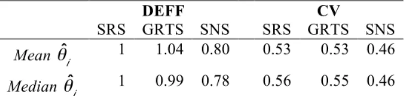
We draw from the census data a simple random sample without replacement, a generalized random tessellation sample and a spatial network sample, each of 225 observations. For each sample design we compute the HT estimator and the Fay-Herriot estimator for the 8 small areas. We replicate this experiment 1000 times. Area sample size varies between simulations and between designs. Performances of the Fay-Herriot estimators under the three different designs are evaluated using the design effect (DEFF) and the coefficient of variation (CV) where the root mean squared error of the estimator has been obtained empirically from simulations. The design effect is evaluated in comparison of the Fay-Herriot estimator under simple random sample. Results are summarized over areas and simulation. In table 1 there is the mean and the median over areas of the DEFF and the CV.

DEFF CV

SRS GRTS SNS SRS GRTS SNS

Mean

!

ˆ

i 1 1.04 0.80 0.53 0.53 0.46

Median

!

ˆ

_i 1 0.99 0.78 0.56 0.55 0.46

Table 1. Mean and median over areas of the design effects (DEFF) and the coefficient of variation (CV) under the simple random sampling (SRS), the generalized random tessellation sampling (GRTS) and the spatial network sampling (SNS)

efficiency of about 20% and shows the smallest coefficients of variations. Further investigations are needed to better assess the performance of this design in small area estimation framework.

References

Cressie, N. (1991). Statistics for spatial data. New York, Wiley.

Fattorini, L. (2006). Applying the Horvitz–Thompson criterion in complex designs: A computer-intensive perspective for estimating inclusion probabilities. Biometrika, 93, 2, 269–278.

Fattorini, L. (2009). An adaptive algorithm for estimating inclusion probabilities and performing the Horvitz–Thompson criterion in complex designs. Computational Statistics 24, 623–639.

Fay R.E. e Herriott R.A. (1979), “Estimates of income for small places: an application of James-Stein procedures to census data”, Journal of the American Statistical Association, 74, 269-277.

Rao J.N.K. (2003), Small Area Estimation, Wiley, New York. Ripley, B.D. (1981). Spatial statistics. New York, Wiley.

Robert, C. P. and Casella, G. (1999). Monte Carlo Statistical Methods. New York: Springer.

Särndal C.E., Swensson B., and Wretman J. (1992). Model Assisted Survey Sampling, Springer Verlag: New York.

Stevens Jr., D.L. and Olsen, A.R. (2003). Variance estimation for spatially balanced samples of environmental resources. Environmetrics, 14, 593–610.

Stevens Jr., D.L. and Olsen, A.R. (2004). Spatially balanced sampling of natural resources. Journal of the American Statistical Association, 99, 262–278.

Traat, I., Bondesson, L., and Meister, K. (2004). Sampling design and sample selection through distribution theory. Journal of Statistical Planning and Inference 123, 395 -413.

Tillé, Y. (2006). Sampling algorithms. Springer series in statistics. Springer, New York.