Hossain, A.; Diaz-Ordaz, K.; Bartlett, J.W. (2016) [Accepted Manuscript] Missing continuous outcomes under covariate dependent missingness in cluster randomised trials. Statistical methods in medical research. ISSN 0962-2802 DOI: https://doi.org/10.1177/0962280216648357
Downloaded from: http://researchonline.lshtm.ac.uk/3615667/
DOI:10.1177/0962280216648357
Usage Guidelines
Please refer to usage guidelines at http://researchonline.lshtm.ac.uk/policies.html or alterna-tively [email protected].
Missing continuous outcomes under covariate
dependent missingness in cluster randomised trials
Anower Hossain
∗1, Karla Diaz-Ordaz
1and Jonathan W. Bartlett
21
Department of Medical Statistics
London School of Hygiene & Tropical Medicine (LSHTM)
2Statistical Innovation Group, AstraZeneca, Cambridge, UK
Abstract
Attrition is a common occurrence in cluster randomised trials (CRTs) which leads to missing outcome data. Two approaches for analysing such trials are cluster-level analysis and individual-level analysis. This paper compares the performance of un-adjusted cluster-level analysis, baseline covariate un-adjusted cluster-level analysis and linear mixed model (LMM) analysis, under baseline covariate dependent missing-ness (CDM) in continuous outcomes, in terms of bias, average estimated standard error and coverage probability. The methods of complete records analysis (CRA) and multiple imputation (MI) are used to handle the missing outcome data. We con-sidered four scenarios, with the missingness mechanism and baseline covariate effect ∗Corresponding author
on outcome either the same or different between intervention groups. We show that both unadjusted cluster-level analysis and baseline covariate adjusted cluster-level analysis give unbiased estimates of the intervention effect only if both intervention groups have the same missingness mechanisms and there is no interaction between baseline covariate and intervention group. LMM and MI give unbiased estimates under all four considered scenarios, provided that an interaction of intervention and baseline covariate is included in the model when appropriate. Cluster mean imputa-tion has been proposed as a valid approach for handling missing outcomes in CRTs. We show that cluster mean imputation only gives unbiased estimates when missing-ness mechanism is the same between the intervention groups and there is no interac-tion between baseline covariate and interveninterac-tion group. MI shows overcoverage for small number of clusters in each intervention group.
1
Introduction
In cluster randomised trials (CRTs), identifiable clusters of individuals such as villages, schools, medical practices - rather than individuals - are randomly allocated to each of intervention and control groups, while individual-level outcomes of interest are observed within each cluster. The number of clusters and/or the cluster sizes in each intervention group might be different. CRTs with equal number of clusters in each intervention group with constant cluster size are known as balanced CRTs. One important characteristic of CRTs is that the outcomes of individuals within the same cluster may exhibit more sim-ilarity compared to the outcomes of individuals in the other clusters, which is quantified by the intraclass correlation coefficient (ICC), denoted by ρ. In practice, the value of
ICC typically ranges form 0.001 to 0.05 and it is rare for clinical outcomes to have ICC above 0.1 [1]. Small values of ICC can lead to substantial variance inflation factors, and should not be ignored [2, 3]. CRTs are being increasingly used in the fields of health promotion and health service research. Reasons for such popularity include the nature of intervention that itself may dictate its application at the cluster level, less risk of in-tervention contamination and administrative convenience [4]. It is well known that the power and precision of CRTs are lower relative to trials that individually randomise the same number of individuals [2]. In spite of this, the advantages associated with CRTs are perceived by researchers to outweigh the potential loss of statistical power and precision in some situations.
Attrition is a common problem for CRTs, leading to missing outcome data. This not only reduces the statistical power of the study, but may result in biased intervention effect estimates [5]. Handling missing data in CRTs is complicated by the fact that data are clustered. Inadequate handling of the missing data may result in misleading inferences [6]. A systematic review [7] revealed that, among all CRTs published in English in 2011, 72% of trials had missing values either in outcomes or in covariates or in both. Among them only 34% of CRTs reported how they handled missing data. One of the reasons may be that the methodological development for dealing with missing data in CRTs has been relatively slow in spite of the increasing popularity of CRTs. Cluster mean imputation has been suggested as a valid approach for handling missing outcome data in CRTs [8].
The impact of missing data on estimation and inference of a parameter of interest de-pends on the missing data mechanism, the method used to handle the missing data, and the choice of statistical methods used for data analysis. In this paper, we study the validity of
three analysis methods - unadjusted cluster-level analysis, adjusted cluster-level analysis and linear mixed model - when there is missingness in the continuous outcome, and this missingness depend on baseline covariates, and conditional on these baseline covariates, not on the outcomes itself. We compare the performance of these methods on complete records and multiply imputed datasets. In addition, we investigate the validity of cluster mean imputation, as proposed by Taljaard [8], under the same missingness assumption.
This paper is organised as follows. Section 2 presents a brief review of the approaches to the analysis of CRTs with complete data. In Section 3, the assumed missingness mech-anism for CRTs is described. Section 4 describes methods of handling missing data in CRTs. In Section 5, we investigate the validity of complete records analysis of CRTs. Section 6 describes a simulation study and presents the results. We conclude the study with some discussion in Section 7.
2
Analysis of CRTs with complete data
We begin by describing the two broad approaches to the analysis of CRTs in the absence of missing data. These are cluster-level analysis and individual-level analysis.
2.1
Cluster-level analysis
Cluster-level analysis can be done in two ways: unadjusted cluster-level analysis and baseline covariate adjusted cluster-level analysis. This approach can be explained as a two-stage process. In the first stage of unadjusted analysis, a relevant summary measure of outcomes is calculated for each cluster. Then, in the second stage, the cluster specific
summary measures of the control and intervention groups obtained in the first stage are compared using appropriate statistical methods. The most common one is the standard
t−test for two independent samples (here referred to as cluster-levelt−test) with degrees of freedom (DF) equal to the total number of clusters in the study minus two. The basis of using this test is that the resulting summary measures are statistically independent, which is a consequence of the clusters being independent of each other. In the case of baseline covariate adjusted analysis, an individual-level regression analysis is carried out at the first stage including all covariates as explanatory variables, except for the intervention indicator, and ignoring the clustering of the data [4, 9]. The individual level residuals from the first-stage model are then used to calculate the cluster-specific summary measures for the control group and the intervention group, which are then compared using cluster-levelt−test in the second stage of analysis to evaluate the intervention effect adjusted for baseline covariates. The main purposes of adjusting for baseline covariates are to increase the credibility of the trial findings by demonstrating that any observed intervention effect is not attributed to the possible imbalance between the intervention groups in term of baseline covariates, and to improve the statistical power [10].
2.2
Individual-level analysis
In individual-level analysis, a regression model is fitted to the individual-level outcomes, allowing for the fact that observations within the same cluster are correlated. Linear mixed model (LMM) is widely used as individual-level analysis for CRTs with continuous out-comes. The LMM takes into account between-cluster variability using cluster-level ef-fects which are assumed to follow a specified probability distribution. The parameters
of that distribution are estimated using maximum likelihood methods together with in-tervention effect and other covariates effects. Generalised estimating equations are an alternative approach, but that for continuous outcomes and an exchangeable correlation matrix, estimates are identical to those from LMM with a random intercept [11].
The adjustedt−test, proposed by Donner and Klar (2000) [2], is a alternative approach to test the intervention effect for quantitative outcomes, which involves calculating the mean of the individual outcome values in each intervention group. These means are then compared using a t−test in which the standard error is adjusted to account for the intra-cluster correlation. The adjustedt−test and the cluster-levelt−test are identical for balanced CRTs.
3
Missingness mechanism assumptions for CRTs
In this paper, we will consider the common setting where the outcomes are continuous, and only outcomes are missing. In statistical analysis, if there are missing values, an assumption must be made about the missingness mechanism, which refers to the rela-tionship between missingness and the underlying values of the variables in the data [12]. According to Rubin’s framework [13], a missingness mechanism can be classified as (i) missing completely at random (MCAR), where the probability of a value being missing is independent of the observed and unobserved data, (ii) missing at random (MAR), where conditioning on the observed data, the probability of a value being missing is independent of the unobserved data, and (iii) missing not at random (MNAR), where the probability of value being missing depends on both observed and unobserved data.
out-comes depends on covariates measured at baseline and conditional on these baseline co-variates, not on the outcome itself. We refer to this as covariate dependent missingness (CDM). For example, blood pressure outcome data could be CDM if missingness in blood pressure measurement depends on covariates (e.g. age, BMI or weight), but given these, not on the blood pressure measurement itself. CDM is an example of a MAR mechanism when covariates are fully observed.
LetYijl be a continuous outcome of interest for thelth(l = 1,2, . . . , mij)individual in thejth (j = 1,2, . . . , ki)cluster of the intervention group i (i = 1,2), where i = 1 corresponds to control group andi = 2 corresponds to intervention group. We assume that theYijlfollow a linear mixed model given by
Yijl =αi +βiXijl+δij +ijl, (3.1)
whereαi is a constant for ith intervention group, Xijl is a baseline covariate value for
(ijl)th individual, βi is the effect of baseline covariate X on Y in intervention group
i, δij is the (ij)th cluster effect and ijl is the individual error term. We also assume that the cluster effect (δij) and the individual error (ijl) are statistically independent; and E(δij) = 0, Var(δij) = σb2 and E(ijl) = 0, Var(ijl) = σ2w, where σb2 and σw2 are the between-cluster variance and within-cluster variance, respectively. Later we will sometimes make normality assumptions on these random effects/random errors. Suppose the baseline covariateXhas meanµx. Then
E Y¯i
whereY¯i = (1/ki)Pkj=1i (1/mij) Pmij
l=1Yijl = (1/ki)Pkj=1i Y¯ij. Here, Y¯i and Y¯ij are the mean outcome of the ith intervention group and the (ij)th cluster, respectively. With complete data, the cluster-level analysis estimate of the intervention effect, sayθˆ, is then calculated as
ˆ
θ= ¯Y1−Y¯2.
With complete data, this estimator is unbiased for the true intervention effect, that is,
E(ˆθ) = µ1−µ2.
Suppose there are some missing values for outcomeY. Define a missing data indicator
Rijlsuch that
Rijl = 1, ifYijl is observed 0, ifYijl is missing. Then Pmij
l=1Rijl is the number of observed outcomes in the (ij)th cluster. The CDM
assumption can then be expressed as
P(Rijl = 0|Yij,Xij) =P(Rijl = 0|Xijl),
whereYij = (Yij1, Yij2, . . . , Yijmij)andXij = (Xij1, Xij2, . . . , Xijmij)are the vectors
of the outcomes and the baseline covariate values, respectively, in the (ij)th cluster. In other words, the missingness of the(ijl)th individual’s outcomeYijldepends only on that individual’s baseline covariate valueXijl.
4
Methods of handling missing data in CRTs
Common approaches for handling missing data in CRTs include complete records analy-sis (CRA), single imputation and multiple imputation (MI). This section describes these approaches. In this paper, we focused on CRA and MI since they are the most commonly used methods for handling missing data.
4.1
Complete records analysis
In complete records analysis (CRA), often referred to as complete case analysis, only individuals with outcome observed are considered in the analysis, while individuals with missing outcome are excluded. It is widely used because of its simplicity and is usually the default method of most statistical packages. It is well known that CRA is valid if data are MCAR or if missingness is independent of the outcome, conditional on covariates [12]. Likelihood based CRA is valid under MAR, if missingness is only in the outcome and all predictors of missingness are conditioned on in the model [12]. CRA is also valid under MNAR mechanisms where missingness in a covariate is dependent on the value of that covariate, but is conditionally independent of outcome [14, 15]
4.2
Single imputation
Single imputation imputes a single value for each missing outcome and creates a complete data set. In general single imputation is not recommended, since estimates of uncertainty are biased downwards, leading to anti-conservative inferences. However, for CRTs two choices for single imputation are group mean imputation and cluster mean imputation [8].
In the first case, missing outcomes in each intervention group are replaced by the mean outcome calculated using complete records pooled across clusters of that group. This approach reduces the variability among the clusters means and, therefore, gives inflated Type I error [8]. In cluster mean imputation, missing outcomes in each cluster are replaced by the mean outcome calculated using complete records of that cluster. This approach has been suggested as a good approach for handling missing outcomes by Taljaard et al. [8]. They showed that cluster mean imputation gives Type I error close to nominal level under MCAR, using adjusted t−test with balanced CRTs. However, under MAR or CDM, adjustedt−test with cluster mean imputation may not be valid. We note that, with balanced CRTs, the cluster-level t−test and the adjusted t−test are identical with cluster mean imputation since after imputation the cluster sizes become constant and the cluster means remain unchanged by the imputation. Consequently, our later results for the validity of cluster level t-test can also be applied to infer the validity of results after using cluster mean imputation. One additional problem with cluster mean imputation is that it distorts the estimates of between-cluster variability and within-cluster variability, which often are of interest.
4.3
Multiple imputation
Multiple imputation (MI), first proposed by Rubin (1987) [16], is a method of filling in the missing outcomes multiple times by simulating from an appropriate model. The aim of imputing multiple times is to allow for the uncertainty about the missing outcomes due to the fact that the imputed values are sampled draws for the missing outcomes. A sequence ofQimputed data sets is obtained by replacing each missing outcome by a set ofQ≥ 2
imputed values that are simulated from an appropriate distribution or model. Each of the
Qdata sets are then analysed as a completed data set using a standard method. The results from theQimputed data sets are then combined using Rubin’s rules [16]. The combined inference is based on at−distribution with DF given by
ν= (Q−1) 1 + Q Q+ 1 WMI BMI 2 , (4.1)
whereBMIis the between-imputation variance andWMIis the average within-imputation
variance. This formula for DF is derived under the assumption that the complete data DF,
νcom, is infinite [17].
In CRTs,νcomis usually small as it is based on the number of clusters in each
inter-vention group rather than the number of individuals. For unadjusted cluster-level analysis and individual-level baseline covariate adjusted cluster-level analysis,νcomis calculated as
k1+k2−2for statistical inference using cluster-levelt−test [4] and adjustedt−test [8]. An
adjustment is made to theνcomto adjust for level baseline covariates using
cluster-level analysis. In this case, we reduce the complete data DF fromνcom = k1 +k2 −2
toνcom = k1 +k2 −2−p, where pis the number of parameters corresponding to the
cluster-level baseline covariates in the first stage regression model [4].
When νcom is small and there is a modest proportion of missing data, the
repeated-imputation DF,ν (given in 4.1), for reference t− distribution can be much higher than
νcom, which is not appropriate [17]. In such a situation, a more appropriate DF, νadj,
proposed by Barnard and Rubin (1999) [17], is calculated as
νadj= 1 ν + 1 ˆ νobs −1 ≤νcom, (4.2)
where ˆ νobs= 1 + Q+ 1 Q BMI WMI −1 νcom+ 1 νcom+ 3 νcom.
At least four different types of MI have been used in CRTs [7]. These arestandard MI which ignores clustering,fixed effects MI which includes a fixed effect for each cluster in the imputation model,random effectsMI where clustering is taken into account through random effects in the imputation model andwithin-clusterMI where standard MI is ap-plied within each cluster. Andridge [18] showed, with balanced CRTs under MCAR and MAR missingness in a continuous outcome with a single covariate in addition to inter-vention indicator, that MI models that incorporate clustering using fixed effects for cluster can result in a serious overestimation of variance of group means and this overestimation is more serious for small cluster sizes and small ICCs. This overestimation of variance results in a decrease in power, which is particularly dangerous for CRTs which are often underpowered [18]. MI using random effects for cluster gave slight overestimation of variance of group means for very small values ofρ. Andridge also showed that using an MI model that ignores clustering can lead to severe underestimation of the MI variance for large values ofρ (>0.005). This underestimation of variance leads to inflated Type I error.
Taljaard et al. [8] examined the performance of MI in a simple set-up considering balanced CRTs where there are no covariates except intervention indicator using stan-dard regression imputation, which ignores clustering, and random effects MI which does account for intraclass correlation. They also considered the Approximate Bayesian Boot-strap (ABB) procedure, proposed by Rubin and Schenker [19], as a non-parametric MI. In ABB, sampling from the posterior predictive distribution of missing data is
approx-imated by first generating a set of plausible contributors drawn with replacement from the observed data, and then imputed values are drawn with replacement from the possi-ble contributors. Two possipossi-ble uses of ABB in CRTs are pooled ABB and within-cluster ABB, where the set of possible contributors are sampled from all observed values across the clusters in each group or from observed values in the same cluster, respectively. They showed that none of these four MI procedures tend to yield better power compared to the power of adjustedt−test using no imputation and cluster mean imputation under MCAR. We note that in the case of missing outcome under MAR for individually randomised trials, Groenwold et al. [20] showed that CRA with covariate adjustment and MI give similar estimates so long as the same set of predictors of missingness are used. It can be anticipated that similar result holds for CRTs. An obvious advantage of CRA over MI is that it is much easier to apply, and therefore in situations where they are equivalent, CRA is clearly preferable.
5
Validity of complete records analyses of CRTs
In this section, we describe the unadjusted cluster-level analysis, baseline covariate ad-justed cluster-level analysis and linear mixed model analysis methods using complete records, and derive conditions under which they give valid inferences under the CDM assumption.
5.1
Unadjusted cluster-level analysis using complete records
The mean of the observed outcomes in theith intervention group can be calculated as
¯ Yiobs= 1 ki ki X j=1 ¯ Yijobs, whereY¯obs ij = 1/ Pmij l=1Rijl Pmij
l=1RijlYijl is the observed mean of (ij)th cluster. The estimate of intervention effect is given by
ˆ
θobs = ¯Y1obs−Y¯2obs. (5.1)
In Appendix A, we show that
E ˆ θobs =µ1−µ2+β1(µx11−µx)−β2(µx21−µx), (5.2) and Varθˆobs= 2 X i=1 1 ki βi2σx2¯ i1 +σ 2 b + σ2 w ηi , (5.3)
whereµxi1 is true mean of the baseline covariateX in theith intervention group among
those individuals with observed outcomes, σx2¯i1 is the variance of the cluster specific means of X among those with observed outcomes, and 1/ηi = E(1/
P
lRijl). From (5.2), it follows that the unadjusted cluster-level analysis using CRA will be unbiased if
β1(µx11−µx) = β2(µx21−µx), or equivalently, β1 β2 = µx21−µx µx11−µx (5.4)
A sufficient condition for (5.4) to hold is thatβ1 =β2(i.e. there is no interaction between
baseline covariate and intervention group in the outcome model) and that the missingness mechanisms are the same in the two intervention groups, so thatµx11 =µx21. It can also
seen from equation (5.2) that, when there is no missing data, µx11 = µx21 = µx, and hence the unadjusted cluster-level analysis results in unbiased estimates of intervention effects even whenβ1 6=β2.
5.2
Adjusted cluster-level analysis using complete records
Recall that the first step of the adjusted cluster-level analysis involves fitting a regression model for Y with X as covariate, but ignoring the intervention indicator and clustering of the data. The residualˆijlis then given by
ˆ
ijl =Yijl−Yˆijl,
whereYˆijl = γ +λXijl is the predicted outcome for the (ijl)th individual based on the first stage model fit. The mean of the observed residuals of theith group is given by
¯ ˆ i obs = 1 ki ki X j=1 ¯ ˆ ij obs , where¯ˆij obs = 1/ Pmij l=1Rijl Pmij
l=1Rijlˆijlis the mean of observed residuals of the(ij)th cluster. The baseline covariate adjusted estimator of intervention effect is given by
ˆ θobsadj = ¯ˆ1 obs −¯ˆ2 obs . (5.5)
We show in Appendix B that E ˆ θobsadj =µ1 −µ2+β1(µx11−µx)−β2(µx21−µx) +λ(µx21−µx11). (5.6)
Hence, the estimator (5.5) will be unbiased if (i) β1 = β2 and µx11 = µx21, or if (ii)
λ = β1 = β2. Equation (5.6 ) is derived (see Appendix B) assuming fixed values of
γandλinstead of their estimates. In practice,γandλare unknown and must be estimated by fitting the first stage regression model for the observed outcomes. We are not worried about the estimate of the intercept parameterγ since the expression (5.6) is independent ofγ. Ifλis estimated consistently, thenθˆobs
adj will be a consistent estimator of intervention
effect when in truthλ = β1 = β2. The estimator of λ, say λˆ, is calculated using
com-plete records, and will be unbiased (and therefore consistent) ifRijl ⊥⊥Yijl|Xijl. This is true only when the two intervention groups have the same missingness mechanisms and have the same baseline covariate effects on outcome in the outcome model. Therefore, assuming CDM, the baseline covariate adjusted cluster-level analysis is consistent only if the two intervention groups have the same covariate effects on outcome in the outcome model and the same missingness mechanisms. We also note that with no missing data
µx11 = µx21 = µx, hence, equation (5.6) guarantees that the adjusted cluster-level
anal-ysis, which assumes that the covariate effect on outcome is the same in both groups, is unbiased, regardless of whether the covariate effect is the same in the intervention groups. The variance of the estimator (5.5) can be written as (see Appendix B for derivation)
Var ˆ θobsadj= 2 X i=1 1 ki (βi−λ)2σ2x¯i1 +σ 2 b + σ2 w ηi . (5.7)
This shows that whenβ1 = β2 and the missingness mechanisms are the same in the two
intervention groups, in order for the estimator(5.5)to have minimum variance one should replace the unknownλby an estimate ofβ1 =β2 =β.
5.3
Linear mixed model using complete records
LetZ be the intervention indicator which is zero for control group and is one for interven-tion group. When it is assumed that the two interveninterven-tion groups have the same covariate effects on outcome, we fit a LMM with fixed effects ofXandZ, and a random effect for cluster. Then the estimate of the coefficient ofZ will be the estimated intervention effect accounting forX.
If one thinks that the baseline covariate effects on outcome could be different in the two intervention groups and there are missing outcome values, an interaction ofX and
Zmust be included in the model. This implies that the intervention effect varies withX. Then the estimate of the intervention effect at the mean value ofX is known as average intervention effect. Let X∗ denote the empirically centred variable X − X¯, where X¯
is the mean of X calculated using data from all individuals. If the baseline covariate effects on outcome are assumed to be different in the two groups, we fit a LMM, using complete records, with fixed effects ofX∗,Zand their interaction, and a random effect for cluster. The estimate of the coefficient ofZwill then be the estimated average intervention effect. One may need to account for the centreing step in the variance estimation. We will investigate in the simulations whether ignoring this has any negative impact on CI coverage.
which are calculated based on their asymptotic distributions, are known to be underesti-mated for small sample sizes [21]. In this paper, we used quantiles fromt−distribution with degrees of freedomk1 +k2 −2rather than the quantiles form the standard normal
distribution to construct the confidence interval for the intervention effect, as this has been used in other papers for individual-level analysis using mixed models for CRTs [22, 23].
6
Simulation Study
A simulation study was conducted to investigate the performance of unadjusted cluster-level analysis, baseline covariate adjusted cluster-cluster-level analysis and LMM using complete records analysis (CRA) under baseline covariate dependent missingness in outcomes. We also investigated whether there is any gain using MI over CRA. The average estimate of intervention effect, its average estimated standard error (SE) and coverage probability were calculated and compared. We considered balanced CRTs, where the two intervention groups have equal number of clusters(ki =k)and constant cluster size(mij =m).
6.1
Data generation and analysis
For each individual in the study a single covariate valueXwas generated independently asX ∼ N(0,1). Sinceσ2
x = 1, we can write the coefficient ofX in (3.1) asβi = τiσy, whereσ2
y is the total variance ofY within each intervention group andτiis the correlation coefficient betweenY andX in intervention groupi. We fixedσ2
α2 = 25. Then the outcomeY was generated using the model
Yijl =αi+τiσyXijl+δij+ijl,
where δij ∼ N(0, ρσ2y) and ijl ∼ N(0,(1− τi2 − ρ)σ2y). We chose the cluster size
m = 30 for each cluster. Parameters that were varied in generating the data include the number of clusters in each group, k = (5,10,20,30) and the unconditional ICC,
ρ = (0.001,0.05,0.1). The missing data indicators Rijl under CDM assumption were generated, independently for each individual, according to a logistic regression model
logit Rijl= 0
Yij,Xij
=φi0+φi1Xijl.
The interceptφi0and slopeφi1were chosen so that Ejl(Rijl) =pi, wherepiis the desired proportion of observed values in intervention groupi. The degree of correlation between missingness and baseline covariate depends on the value ofφi1. We usedφ11 =φ21 = 1,
which gives the odds ratio for having a missing outcome(Y) is 2.72 associated with a one unit increase in the covariate(X)value. Missing data indicators were then imposed to each generated complete data to get the incomplete data.
Four possible scenarios were considered:
1. φ10 =φ20 =−1andτ1 =τ2 = 0.5: missingness mechanism is the same between
the intervention groups and there is no interaction between intervention group and baseline covariate in the outcome model.
2. φ10 = −1, φ20 = 0.5 and τ1 = τ2 = 0.5: missingness mechanism is different
group and baseline covariate in the outcome model.
3. φ10 = φ20 = −1 and τ1 = 0.4, τ2 = 0.6 : missingness mechanism is the same
between the intervention groups and there is an interaction between intervention group and baseline covariate in the outcome model.
4. φ10=−1, φ20 = 0.5andτ1 = 0.4, τ2 = 0.6: missingness mechanism is different
between the intervention groups and there is an interaction between intervention group and baseline covariate in the outcome model.
In the first and third scenarios, there was 30% missing outcomes in both the inter-vention groups. In the second and fourth scenarios, there was 30% missing outcomes in the control group, and 60% missing outcomes in the intervention group. Each generated incomplete data set was then analysed using unadjusted cluster-level analysis, baseline covariate adjusted cluster-level analysis and LMM using complete records. We included the interaction between intervention and covariate into the LMM in the third and fourth scenarios, where the two intervention groups have different covariate effects on outcome in the data generating model for outcome.
The R package jomo [24] was used to multiply impute each generated incomplete data set using MI with number of imputations 20. A random intercept LMM was used as the imputation model so that the imputation model was correctly specified. We used 200 burn-in iterations and 10 iterations between two successive draws after examining, respectively, the convergence of the posterior distributions of the parameters estimates of the imputation model and the plots of their autocorrelation functions. The completed data sets were then analysed using LMM. An interaction between intervention and baseline
covariate was included in both the imputation model and the analysis model when the two intervention groups have different covariate effects on outcome in the data generating model. We always used restricted maximum likelihood estimation method to fit the LMM. The Waldt−test with adjusted DF, given in equation 4.2, withνcom = 2(k−1)was used to
test the null hypothesis of intervention effect. We had maximum 50 convergence warnings in 10,000 simulations when LMM was fitted using the R packagelme4[25].
6.2
Results
Empirical average estimates of intervention effect, average estimated standard errors (SEs) and coverage probabilities of nominal 95% confidence interval over 10000 simulation runs for each of the four scenarios are presented in Tables 1 to 4, respectively.
When the missingness mechanism is the same between the intervention groups and there is no interaction between intervention and baseline covariate in the outcome model, both the unadjusted and adjusted cluster-level analyses gave unbiased estimates of inter-vention effect with coverage probabilities very close to the nominal level (see Table 1). However, these two methods gave biased estimates of intervention effect if the two inter-vention groups had either different missingness mechanisms or there was an interaction between intervention and covariate in the outcome model or both (see Table 2, Table 3 and Table 4, respectively). These results support our derived conditions explained in Sec-tion 5.1 and SecSec-tion 5.2, respectively, for unadjusted and adjusted cluster-level analyses to be unbiased using CRA, where we showed that these two methods are unbiased only if the missingness mechanism is the same between the intervention groups and there is no interaction between intervention and baseline covariate in the data generating model
T able 1: Simulation results-missingness mechanism is the same between the interv ention groups and there is no interaction between interv ention and baseline co v ariate in the data generating model for outcome. Empirical av erage estimates of interv ention ef fect, av erage estimated SEs and co v erage probabilities of nominal 95% confidence interv al o v er 10000 simulation runs for unadjusted cluster -le v el analysis (CL(unadj)), baseline co v ariate adjusted cluster -le v el analysis (CL(adj)), linear mix ed model (LMM), using CRA, and multiple imputation (MI). Monte-Carlo errors for av erage estimates and av erage estimat ed SEs are all less than 0.023 and 0.016, respecti v ely . The true v alue of the interv ention ef fect is 5. ρ k A v erage Estimate A v erage estimated SE Co v erage (%) CL(unadj) CL(adj) LMM MI CL(unadj) CL(adj) LMM MI CL(unadj) CL(adj) LMM MI 0.1 5 4.98 4.99 4.99 4.98 2.31 2.21 2.23 2.19 95.2 95.1 95.2 96.3 10 5.01 4.98 5.00 4.99 1.66 1.59 1.60 1.59 95.1 95.3 95.3 95.5 20 4.99 4.99 4.99 4.99 1.18 1.14 1.14 1.14 94.9 95.0 94.9 94.8 30 5.01 5.00 5.01 5.01 0.97 0.93 0.93 0.93 95.0 95.0 94.9 95.0 0.05 5 5.00 4.98 5.00 5.00 1.88 1.76 1.78 1.76 95.2 95.1 95.6 96.2 10 5.01 5.00 5.01 5.01 1.35 1.28 1.28 1.26 95.1 95.2 95.1 95.4 20 5.01 5.00 5.01 5.01 0.96 0.91 0.91 0.90 95.0 95.0 95.1 95.0 30 4.99 4.99 4.99 4.99 0.79 0.75 0.74 0.74 95.0 95.0 95.0 95.0 0.001 5 4.98 4.98 4.99 4.99 1.34 1.18 1.31 1.35 95.2 95.1 96.2 99.6 10 5.01 5.00 5.01 5.01 0.96 0.85 0.90 0.93 95.1 95.1 96.8 97.8 20 4.99 4.99 5.00 5.00 0.69 0.61 0.63 0.64 94.8 94.9 96.2 96.7 30 5.00 5.00 5.00 5.00 0.56 0.50 0.51 0.52 95.1 95.3 96.2 96.8
T able 2: Simulation results-missingness mechanism is dif ferent between the interv ention groups and there is no interaction between interv ention and baseline co v ariate in the data generating model for outcome. Empirical av erage estimates of interv ention ef fect, av erage estimated SEs and co v erage probabilities of nominal 95% confidence interv al o v er 10000 simulation runs for unadjusted cluster -le v el analysis (CL(unadj)), baseline co v ariate adjusted cluster -le v el analysis (CL(adj)), linear mix ed model (LMM), using CRA, and multiple imputation (MI). Monte-Carlo errors for av erage estimates and av erage estimat ed SEs are all less than 0.025 and 0.017, respecti v ely . The true v alue of the interv ention ef fect is 5. ρ k A v erage Estimate A v erage estimated SE Co v erage (%) CL(unadj) CL(adj) LMM MI CL(unadj) CL(Adj) LMM MI CL(unadj) CL(Adj) LMM MI 0.1 5 3.83 4.94 5.01 5.01 2.44 2.32 2.34 2.28 93.2 95.1 95.2 97.0 10 3.81 4.94 5.03 5.03 1.76 1.67 1.68 1.66 89.9 95.4 95.2 95.5 20 3.78 4.91 5.00 4.99 1.25 1.19 1.19 1.19 84.2 94.9 94.8 94.8 30 3.79 4.93 5.01 5.01 1.02 0.98 0.98 0.98 79.1 95.4 95.3 95.4 0.05 5 3.77 4.90 4.98 4.98 2.04 1.90 1.94 1.92 91.7 94.9 95.7 98.3 10 3.78 4.90 5.00 4.99 1.48 1.38 1.38 1.36 87.5 95.0 95.0 95.8 20 3.76 4.92 4.98 4.98 1.05 0.98 0.98 0.97 79.4 95.2 95.1 95.1 30 3.77 4.92 4.99 4.99 0.86 0.80 0.80 0.80 70.7 94.8 94.6 94.7 0.001 5 3.77 4.89 5.00 5.00 1.58 1.39 1.54 1.60 89.4 95.1 98.3 99.7 10 3.76 4.89 4.99 4.98 1.14 1.01 1.06 1.10 82.1 95.0 97.3 98.5 20 3.78 4.91 5.00 5.00 0.81 0.72 0.74 0.76 68.8 95.2 96.4 97.3 30 3.78 4.92 5.00 5.00 0.66 0.59 0.60 0.61 56.1 94.9 95.8 96.5
T able 3: Simulation results-missingness mechanism is the same between the interv ention groups and there is an interaction between interv ention and baseline co v ariate in the data generating model for outcome. Empirical av erage estimates of interv ention ef fect, av erage estimated SEs and co v erage probabilities of nominal 95% confidence interv al o v er 10000 simulation runs for unadjusted cluster -le v el analysis (CL(unadj)), baseline co v ariate adjusted cluster -le v el analysis (CL(adj)), linear mix ed model (LMM), using CRA, and multiple imputation (MI). Monte-Carlo errors for av erage estimates and av erage estimat ed SEs are all less than 0.024 and 0.016, respecti v ely . The true v alue of the interv ention ef fect is 5. ρ k A v erage Estimate A v erage estimated SE Co v erage (%) CL(unadj) CL(adj) LMM MI CL(unadj) CL(Adj) LMM MI CL(unadj) CL(Adj) LMM MI 0.1 5 4.46 4.44 4.97 4.97 2.31 2.22 2.25 2.22 94.3 94.3 95.0 96.4 10 4.50 4.49 5.01 5.02 1.66 1.59 1.61 1.60 93.7 93.6 94.7 94.8 20 4.48 4.48 5.00 5.00 1.19 1.14 1.15 1.15 92.5 92.6 94.9 94.9 30 4.49 4.49 5.00 5.00 0.97 0.93 0.94 0.94 91.3 91.2 94.7 94.7 0.05 5 4.45 4.43 4.96 4.97 1.88 1.76 1.81 1.80 94.0 93.7 95.3 97.1 10 4.51 4.49 5.01 5.01 1.36 1.28 1.30 1.29 93.7 93.4 95.0 95.5 20 4.50 4.50 5.01 5.01 0.97 0.91 0.92 0.92 91.9 91.6 94.8 94.8 30 4.50 4.50 5.01 5.01 0.79 0.75 0.76 0.75 90.4 89.8 94.6 94.6 0.001 5 4.48 4.46 4.99 4.99 1.34 1.18 1.35 1.39 93.4 93.5 98.1 99.4 10 4.50 4.49 5.02 5.01 0.96 0.85 0.93 0.96 92.3 91.6 96.9 97.9 20 4.49 4.49 5.00 5.00 0.69 0.61 0.65 0.66 88.9 87.2 96.3 96.8 30 4.48 4.48 4.99 4.99 0.56 0.50 0.52 0.54 84.9 81.6 95.6 96.3
T able 4: Simulat ion results-missingness mechanism is dif ferent between the interv ention groups and there is an interaction between interv ention and baseline co v ariate in the data generating model for outcome. Empirical av erage estimates of interv ention ef fect, av erage estimated SEs and co v erage probabilities of nominal 95% confidence interv al o v er 10000 simulation runs using unadjusted cluster -le v el analysis (CL(unadj)), baseline co v ariate adjusted cluster -le v el analysis (CL(Adj)), linear mix ed model (LMM), using CRA, and mult iple imputation (MI). Monte-Carlo errors for av erage estimates and av erage estimated SEs are all less than 0.025 and 0.018, respecti v ely . The true v alue of the interv ention ef fect is 5. ρ k A v erage Estimate A v erage estimated SE Co v erage (%) CL(unadj) CL(adj) LMM MI CL(unadj) CL(Adj) LMM MI CL(unadj) CL(Adj) LMM MI 0.1 5 3.02 4.09 5.00 5.00 2.44 2.31 2.42 2.37 89.0 93.4 95.7 98.1 10 3.03 4.10 5.01 5.01 1.76 1.67 1.73 1.71 82.0 93.5 95.8 96.3 20 3.03 4.11 5.01 5.01 1.25 1.19 1.23 1.23 66.6 88.8 95.6 95.6 30 3.03 4.11 5.01 5.02 1.02 0.97 1.01 1.01 52.8 85.9 95.2 95.2 0.05 5 3.02 4.10 5.01 5.01 2.05 1.89 2.06 2.04 87.0 93.9 96.5 99.0 10 3.02 4.10 5.01 5.01 1.47 1.36 1.45 1.44 75.9 90.4 95.7 96.7 20 3.01 4.08 4.98 4.98 1.05 0.98 1.03 1.03 55.3 84.9 95.8 95.9 30 3.02 4.10 5.01 5.00 0.86 0.80 0.84 0.84 38.0 81.1 95.6 95.7 0.001 5 3.02 4.07 4.99 4.99 1.57 1.37 1.69 1.75 80.4 91.1 98.5 99.8 10 3.03 4.10 5.00 5.00 1.13 0.99 1.17 1.21 63.0 87.6 97.6 98.7 20 3.02 4.10 5.00 5.00 0.81 0.71 0.81 0.84 33.4 77.7 97.0 97.7 30 3.01 4.10 5.00 5.00 0.66 0.58 0.66 0.68 16.7 67.9 96.5 97.1
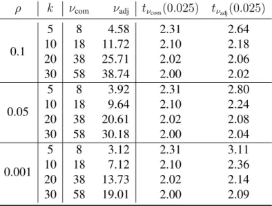
Table 5: Comparison between the complete data DF(νcom)and the average estimates of
adjusted DF (νadj), over 10000 simulation runs, used by MI, when the two intervention
groups have different missingness mechanisms and different covariate effects on outcome in the data generating model for outcome (scenario 4). The last two columns show the upper 2.5% points of thet−distribution withνcomandνadjDF, respectively.
ρ k νcom νadj tνcom(0.025) tνadj(0.025)
0.1 5 8 4.58 2.31 2.64 10 18 11.72 2.10 2.18 20 38 25.71 2.02 2.06 30 58 38.74 2.00 2.02 0.05 5 8 3.92 2.31 2.80 10 18 9.64 2.10 2.24 20 38 20.61 2.02 2.08 30 58 30.18 2.00 2.04 0.001 5 8 3.12 2.31 3.11 10 18 7.12 2.10 2.36 20 38 13.73 2.02 2.14 30 58 19.01 2.00 2.09
for the outcome. These results also imply that cluster mean imputation, as proposed by Taljaard [8] (described in Section 4.2 ), is not valid under CDM assumption unless the two intervention groups have the same missingness mechanisms and there is no inter-action between intervention and baseline covariate in the outcome model. The bias in average intervention effect estimates could be in either direction. But, in this paper, we always have downward bias in the reported intervention effect estimates. This is because we considered a positive correlation between baseline covariate and outcome in the data generation process, and a positive association between baseline covariate and probability of missingness in outcomes. As a result, a large value of outcome has higher chance of being missing compared to a low value of outcome. In our simulations the degree of bias was high if the two intervention groups had different covariate effects on outcome and
it goes up if, in addition, the two intervention groups have different missingness mecha-nisms (see Table 3 and Table 4). LMM and MI gave unbiased estimates of intervention effect under all the four considered scenarios, provided that an interaction of intervention and baseline covariate was included in the model to allow for different covariate effects on outcome in the two intervention groups (scenario 3 and 4).
The LMM and MI had similar empirical average estimated standard errors of the in-tervention effect estimates. The LMM gave coverage probabilities close to nominal level except for very smallρ and small k, where it showed slightly overcoverage. However, while LMM with νcom gave good coverage, MI using νadj gave overcoverage, and this
can be attributed to it used a smaller DF. The average estimates ofνadj, used by MI, over
10,000 simulations runs andνcomfor scenario 4 are presented in Table 5. Results showed
that the estimates ofνadjare smaller compared toνcom.
7
Discussion and Conclusion
In this paper, we aimed to investigate the validity of the unadjusted and adjusted cluster-level analyses, and linear mixed model for analysing CRTs, where the outcomes are con-tinuous and only outcomes are missing under covariate dependent missingness assump-tion. We used complete records analysis and multiple imputation for handling the missing outcomes. The contributions of the paper can be summarised as follows:
First, we found that both the unadjusted and adjusted cluster-level analyses are in gen-eral biased using CRA unless there is no interaction between intervention and baseline covariate in the data generating model for outcome; and the missingness mechanism is the same between the interventions groups, which is arguably unlikely to hold in practice.
Cluster-level analysis is used by many researcher to analyse CRTs because of its sim-plicity. We therefore caution researchers that these methods may commonly give biased inferences in CRTs with missing outcomes. However, we note that these two methods are unbiased with full data, even when there is an interaction between baseline covariate and intervention in the true data generating model for outcome.
Second, cluster mean imputation has been previously recommended as a valid ap-proach for handling missing outcomes in CRTs. We found that cluster mean imputation gave invalid inferences under covariate dependent missingness assumption unless miss-ingness mechanism is the same between the intervention groups and there is no interaction between intervention and baseline covariate in the data generating model for outcome.
Third, the LMM using CRA gave unbiased estimates of intervention effect regardless of whether missingness mechanisms are the same or are different between the intervention groups and whether there is an interaction between intervention and baseline covariate in the data generating model for the outcome, provided that an interaction between inter-vention and baseline covariate was included in the model when such interaction exists in truth.
Finally, we compared the results of LMM using CRA with the results of MI. As expected, we found that MI gave unbiased intervention effects estimates regardless of whether missingness mechanisms are the same or are different in the two intervention groups and whether there is an interaction between intervention and baseline covariate. The LMM and MI had similar empirical standard errors of the estimates of intervention effects. However, MI using adjusted degrees of freedom estimates gave overcoverage for the nominal 95% confidence interval. This is due to underestimation of adjusted degrees
of freedom used by MI compared to complete data degrees of freedom. Groenwoldet al.
[20] showed that that there is little to be gained by using MI over LMM in the absence of auxiliary variables. Moreover, when missingness is confined to outcomes, LMM fitted using maximum likelihood are fully efficient and valid under MAR.
Throughout this paper, we have assumed covariate dependent missingness mechanism in a continuous outcome, which is an example of MAR as our baseline covariate was fully observed. In practice, we cannot identify on the basis of the observed data which missingness assumption is appropriate [14, 26]. Therefore, sensitivity analyses should be performed [26, Ch. 10] to explore whether our inferences are robust to the primary working assumption regarding the missingness mechanism. Furthermore, we focused on studies with only one individual-level covariate; the methods described can be extended for more than one covariates.
In conclusion, in the absence of auxiliary variables, LMM can be recommended as the primary analysis approach for CRTs with missing outcomes if one is willing to make baseline covariate dependent missingness assumption for outcomes.
Appendices
A
Unadjusted cluster-level analysis using CRA
The mean of the observed outcomes in a particular cluster can be written as
¯ Yijobs = Pmij1 l Rijl mij X l=1 RijlYijl = P1 lRijl mij X l=1
Rijl(αi+βiXijl+δij +ijl)
= αi+βi 1 P lRijl mij X l=1 RijlXijl+δij+ 1 P lRijl mij X l=1 Rijlijl = αi+βiX¯ijobs+δij + 1 P lRijl mij X l=1 Rijlijl, whereX¯obs ij = (1/ P lRijl) Pmij
l=1RijlXijl is the observed mean of the baseline covariate
Xin the(ij)th cluster. The expected value ofX¯obs
ij across the clusters in theith interven-tion group will be the true mean ofX among those individuals with observed outcomes. Letµxi1 denote the true mean of the baseline covariate X in theith intervention group
among those individuals with observed outcomes. Then
E Y¯ijobs=αi+βiµxi1+E 1 P lRijl mij X l=1 Rijlijl !
LetRij = (Rij1, Rij2, . . . , Rijmij)be the vector of missing data indicators for the(ij)th cluster. Then E P1 lRijl mij X l=1 Rijlijl ! = E " E P1 lRijl mij X l=1 Rijlijl Rij !# = E " 1 P lRijl mij X l=1 RijlE ijl Rij # = 0, (A.1)
sinceijl’s are independent ofRijl’s and E(ijl) = 0. Therefore, we have
E Y¯ijobs=αi+βiµxi1.
The variance ofY¯ij can be written as
Var Y¯ijobs = βi2Var X¯ijobs +σb2+Var P1 lRijl mij X l=1 Rijlijl ! = βi2σx2¯i1 +σ2b +Var P1 lRijl mij X l=1 Rijlijl ! , σ2 ¯
xi1 is the variance of the cluster specific means of X among those with observed out-comes.
Now Var Pmij1 l Rijl mij X l=1 Rijlijl ! = Var " E P1 lRijl miij X l=1 Rijlijl Rij !# +E " Var P1 lRijl mij X l=1 Rijlijl Rij !# = 0 +E " 1 (P lRijl) 2 mij X l=1 RijlVar ijl Rij # , using (A.1) = σw2E 1 P lRijl = σ 2 w ηi , (A.2) where E 1/ Pmij l Rijl = 1/ηi (say) . Therefore, Var Y¯ijobs =βi2σx2¯ i1 +σ 2 b + σ2 w ηi .
The observed mean of theith intervention group is calculated as
¯ Yiobs = 1 ki ki X j=1 ¯ Yijobs Then E Y¯iobs=αi+βiµxi1. and Var Y¯iobs = 1 ki βi2σx2¯ i1 +σ 2 b + σ2 w ηi .
values is given by
ˆ
θobs = ¯Y1obs−Y¯2obs.
Then E ˆ θobs = (α1 +β1µx11)−(α2+β2µx21) = (α1 +β1µx)−(α2+β2µx) +β1(µx11−µx)−β2(µx21−µx) = µ1−µ2+β1(µx11−µx)−β2(µx21−µx). and Varθˆobs = 1 k1 β12σx112¯ +σb2+σ 2 w η1 + 1 k2 β22σx212¯ +σb2+ σ 2 w η2 = 2 X i=1 1 ki βi2σx2¯ i1 +σ 2 b + σ2 w ηi ,
B
Adjusted cluster-level analysis using CRA
The mean of observed residuals of a particular cluster is given by
¯ ˆ ij obs = Pmij1 l Rijl mij X l=1 Rijlˆijl = P1 lRijl mij X l=1 Rijl Yijl−Yˆijl = P1 lRijl mij X l=1
Rijl(αi+βiXijl+δij +ijl−γ−λXijl)
= αi+ (βi−λ) 1 P lRijl mij X l=1 RijlXijl+δij + 1 P lRijl mij X l=1 Rijlijl−γ = αi+ (βi−λ) ¯Xijobs+δij + 1 P lRijl mij X l=1 Rijlijl−γ Then E ¯ ˆ ij obs =αi+ (βi−λ)µxi1−γ and Var ¯ ˆ ij obs = (βi−λ)2σx2¯i1 +σ 2 b + σ2 w ηi ,
using the results (A.1) and (A.2). The mean of observed residuals of theith intervention group can be written as
¯ ˆ i obs = 1 ki ki X j=1 ¯ ˆ ij obs Then E¯ˆi obs =αi + (βi−λ)µxi1−γ
and Var¯ˆi obs = 1 ki (βi−λ) 2 σx2¯i1 +σb2+σ 2 w ηi .
The baseline covariate adjusted estimator of intervention effect, based on observed values, is given by ˆ θadjobs= ¯ˆ1 obs −¯ˆ2 obs Then Eθˆadjobs = (α1 + (β1−λ)µx11−γ)−(α2+ (β2−λ)µx21−γ) = (α1 +β1µx)−(α2 +β2µx) +β1(µx11−µx)−β2(µx21−µx) +λ(µx21−µx11) = µ1−µ2+β1(µx11−µx)−β2(µx21−µx) +λ(µx21−µx11) and
Varθˆadjobs = 1
k1 (β1−λ) 2 σx112¯ +σb2+σ 2 w η1 + 1 k2 (β2−λ) 2 σx212¯ +σb2+σ 2 w η2 = 2 X i=1 1 ki (βi−λ) 2 σx2¯i1 +σ2b + σ 2 w ηi
which tends to zero as(k1, k2)tend to infinity.
C
List of Abbreviations
ABB Approximate Bayesian Bootstrap
CL(adj) Adjusted Cluster-level Analysis
CL(unadj) Unadjusted Cluster-level Analysis
CRA Complete Records Analysis
CRTs Cluster Randomised Trials
DF Degrees of Freedom
ICC Intraclass Correlation Coefficient
LMM Linear Mixed Model
MAR Missing At Random
MCAR Missing Completely At Random
MI Multiple Imputation
MNAR Missing Not At Random
Acknowledgements
The authors thank the anonymous reviewers for their comments and constructive sugges-tions which led to an improvement over the earlier version of the manuscript.
Funding
A Hossain was supported by the Economic and Social Research Council (ESRC), UK, via Bloomsbury Doctoral Training Centre (ES/J5000021/1). K Diaz-Ordaz was funded by Medical Research Council (MRC) career development award in Biostatistics (MR/L011964/1). J W Bartlett was supported by MRC fellowship (MR/K02180X/1) while a member of the Department of Medical Statistics, London School of Hygiene & Tropical Medicine (LSHTM).
References
[1] Murray DM, Blitstein JL. Methods to reduce the impact of interclass correlation in group-randomised trials. Evaluation Review. 2003;27:79–103.
[2] Donner A, Klar N. Design and Analysis of Cluster Randomization Trials in Health Research. Arnold, London; 2000.
[3] Murray DM. Design and Analysis of Group- Randomized Trials. Oxford University Press, New York; 1998.
[4] Hayes RJ, Moulton LH. Cluster Randomised Trials. CRC Press, Taylor & Francis Group; 2009.
[5] Wood AM, White IR, Thompson SG. Are missing outcome data adequately han-dled? A review of published randomized controlled trials in major medical journals. Clinical Trials. 2004;1(4):368–376.
[6] Sterner JA, White IR, Carlin JB, Spratt M, Royston P, Kenward MG, et al. Multiple imputation for missing data in epidemiological and clinical research: potential and pitfalls. BMJ. 2009;339:157–160.
[7] Diaz-Ordaz K, Kenward MG, Cohen A, Coleman CL, Eldridge S. Are missing data adequately handled in cluster randomised trials? A systematic review and guide-lines. Clinical Trials. 2014;11(5):590–600.
[8] Taljaard M, Donner A, Klar N. Imputation Strategies for Missing Continuous Out-comes in Cluster Randomized Trials. Biometrical journal. 2008;50(3):329–345. [9] Gail MH, Tan WY, Piantadosi S. Tests for no treatment effect in randomised clinical
trials. Biometrika. 1988;75(1):57–64.
[10] Hernandez AV, Steyerberg EW, Habbema JD. Covariate adjustment in randomized controlled trials with dichotomous outcomes increases statistical power and reduces sample size requirements. Journal of Clinical Epidemiology. 2004;57(5):454–460. [11] Hubbard AE, Ahern J, Fleischer NL, Van der Laan M, Lippman SA, Jewell N, et al.
To GEE or not to GEE: comparing population average and mixed models for estimat-ing the associations between neighborhood risk factors and health. Epidemiology. 2010;21(4):467–474.
[12] Little RJA, Rubin DB. Statistical Analysis with Missing Data. 2nd Edition. John Wiley & Sons, New Jersey.; 2002.
[14] White IR, Carlin JB. Bias and efficiency of multiple imputation compared with complete-case analysis for missing covariate values. Statistics in Medicine. 2010;29(28):2920–2931.
[15] Bartlett JW, Carpenter JR, Tilling K, Vansteelandt S. Improving upon the ef-ficiency of complete case analysis when covariates are MNAR. Biostatistics. 2014;15(4):719–730.
[16] Rubin DB. Multiple Imputation for Nonresponse in Surveys. John Wiley & Sons , New York; 1987.
[17] Barnard J, Rubin DB. Small-sample degrees of freedom with multiple imputation. Biometrika. 1999;86(4):948–955.
[18] Andridge RR. Quantifying the impact of fixed effects modeling of clusters in multi-ple imputation for cluster randomized trials. Biometrical Journal. 2011;53(1):57–74. [19] Rubin DB, Schenker N. Multiple imputation for interval estimation from simple random samples with ignorable nonresponses. Journal of the American Statistical Association. 1986;81(394):366–374.
[20] Groenwold RH, Donders AR, Roes KC, Harrell FE, Moons KG. Dealing with miss-ing outcome data in randomized trials and observational studies. American Journal of Epidemiology. 2012;175(3):210–217.
[21] Kenward MG, Roger JH. Small sample inference for fixed effects from restricted maximum likelihoods. Biometrics. 1997;53:983–997.
[22] Ukoumunne OC, Carlin JB, Gulliford MC. A simulation study of odds ratio esti-mation for binary outcomes from cluster randomized trials. Statistics in Medicine. 2007;26(18):3415–3428.
[23] Ma J, Thabane L, Kaczorowski J, Chambers L, Dolovich L, Karwalajtys T, et al. Comparison of Bayesian and classical methods in the analysis of cluster randomized controlled trials with a binary outcome: the Community Hypertension Assessment Trial (CHAT). BMC Medical Research Methodology. 2009;9:37.
[24] Quartagno M, Carpenter J. jomo: A package for Multilevel Joint Modelling Mul-tiple Imputation; 2015. Available from: http://CRAN.R-project.org/ package=jomo.
[25] Bates D, Maechler M, Bolker B, Walker S. lme4: Linear mixed-effects models us-ing Eigen and S4; 2014. Available from: http://CRAN.R-project.org/ package=lme4.
[26] Carpenter JR, Kenward MG. Multiple Imputations and its Applications. John Wiley & Sons; 2013.