Memorial Sloan-Kettering Cancer Center
Memorial Sloan-Kettering Cancer Center, Dept. of Epidemiology
& Biostatistics Working Paper Series
Year Paper
Integrative Clustering of Multiple Genomic
Data Types using a Joint Latent Variable
Model with Application to Breast and Lung
Cancer Subtype Analysis
Ronglai Shen
∗Adam Olshen
†Marc Ladanyi
‡∗Memorial Sloan-Kettering Cancer Center, Dept. of Epidemiology and Biostatistics,
†Memorial Sloan-Kettering Cancer Center, Dept. of Epidemiology and Biostatistics,
‡Memorial Sloan-Kettering Cancer Center, Dept. of Pathology, [email protected]
This working paper is hosted by The Berkeley Electronic Press (bepress) and may not be commer-cially reproduced without the permission of the copyright holder.
http://biostats.bepress.com/mskccbiostat/paper18
Integrative Clustering of Multiple Genomic
Data Types using a Joint Latent Variable
Model with Application to Breast and Lung
Cancer Subtype Analysis
Ronglai Shen, Adam Olshen, and Marc Ladanyi
Abstract
The molecular complexity of a tumor manifests itself at the genomic, epige-nomic, transcriptomic, and proteomic levels. Genomic profiling at these multi-ple levels should allow an integrated characterization of tumor etiology. How-ever, there is a shortage of effective statistical and bioinformatic tools for truly integrative data analysis. The standard approach to integrative clustering is sep-arate clustering followed by manual integration. A more statistically powerful approach would incorporate all data types simultaneously and generate a sin-gle integrated cluster assignment. We developed a joint latent variable model for integrative clustering. We call the resulting methodology iCluster. iCluster incorporates flexible modeling of the associations between different data types and the variance-covariance structure within data types in a single framework, while simultaneously reducing the dimensionality of the data sets. Likelihood-based inference is obtained through the Expectation-Maximization algorithm. We demonstrate the iCluster algorithm using two examples of joint analysis of copy number and gene expression data, one from breast cancer and one from lung can-cer. In both cases, we identified subtypes characterized by concordant DNA copy number changes and gene expression as well as unique profiles specific to one or the other in a completely automated fashion. In addition, the algorithm dis-covers potentially novel subtypes by combining weak yet consistent alteration patterns across data types. R code to implement iCluster can be downloaded at http://www.mskcc.org/mskcc/html/85130.cfm.
Integrative Clustering of Multiple Genomic Data Types
using a Joint Latent Variable Model with Application to
Breast and Lung Cancer Subtype Analysis
Ronglai Shen
Department of Epidemiology and Biostatistics,
Memorial Sloan-Kettering Cancer Center, New York, NY 10065, U.S.A.
Adam B. Olshen
Department of Epidemiology and Biostatistics and Helen Diller Family Comprehensive Cancer Center, University of California, San Francisco, CA 94143, U.S.A.,
Marc Ladanyi
Department of Pathology and Human Oncology and Pathogenesis Program, Memorial Sloan-Kettering Cancer Center, New York, NY 10065, U.S.A.
Abstract
The molecular complexity of a tumor manifests itself at the genomic, epigenomic, transcriptomic, and proteomic levels. Genomic profiling at these multiple levels should allow an integrated characterization of tumor etiology. However, there is a shortage of effective statistical and bioinformatic tools for truly integrative data analysis. The standard approach to integrative clustering is separate clustering followed by manual integration. A more statistically powerful approach would incorporate all data types simultaneously and generate a single integrated cluster assignment. We developed a joint latent variable model for integrative clustering. We call the resulting methodology
iCluster. iCluster incorporates flexible modeling of the associations between different
data types and the variance-covariance structure within data types in a single frame-work, while simultaneously reducing the dimensionality of the data sets. Likelihood-based inference is obtained through the Expectation-Maximization algorithm. We demonstrate the iCluster algorithm using two examples of joint analysis of copy num-ber and gene expression data, one from breast cancer and one from lung cancer. In both cases, we identified subtypes characterized by concordant DNA copy number changes
and gene expression as well as unique profiles specific to one or the other in a completely automated fashion. In addition, the algorithm discovers potentially novel subtypes by combining weak yet consistent alteration patterns across data types. R code to imple-ment iCluster can be downloaded at http://www.mskcc.org/mskcc/html/85130.cfm.
1
Introduction
In recent years genomic profiling of multiple data types in the same set of tumors has gained prominence. In a breast cancer study relating DNA copy number to gene expression,
Pol-lack et al. (2002) estimated that 62% of highly amplified genes demonstrate moderately or
highly elevated gene expression, and that DNA copy number aberrations account for about 10-12% of the global gene expression changes at the messenger RNA (mRNA) level. Hyman
et al.(2002) observed similar results in breast cancer cell lines. MicroRNAs, which are small
noncoding RNAs that repress gene expression by binding mRNA target transcripts, provide another mechanism of gene expression regulation. Over 1000 microRNAs are predicted to exist in humans, and they are estimated to target one-third of all genes in the genome (Lewis
et al., 2005). The NCI/NHGRI-sponsored Cancer Genome Atlas (TCGA) pilot project is a
coordinated effort to explore the entire spectrum of genomic alternations in human cancer to obtain an integrated view of such interplays. The group recently published an interim analysis of DNA sequencing, copy number, gene expression and DNA methylation data in a large set of glioblastomas (TCGA, 2008).
In this study, we will refer to any genomic data set involving more than one data type measured in the same set of tumors as multiple genomic platform (MGP) data. Identify-ing tumor subtypes by simultaneously analyzIdentify-ing MGP data is a new problem. The current approach to subtype discovery across multiple types is to separately cluster each type and then to manually integrate the results. An ideal integrative clustering approach would allow joint inference from MGP data and generate a single integrated cluster assignment through simultaneously capturing patterns of genomic alterations that are: 1) consistent across mul-tiple data types; 2) specific to individual data types; or 3) weak yet consistent across data sets that would emerge only as a result of combining levels of evidence. Therefore, the goal of this study is to develop such an integrative framework for tumor subtype discovery.
There are two major challenges to the development of a truly integrative approach. First, to capture both concordant and unique alterations across data types, separate modeling of the covariance between data types and the variance-covariance structure within data types is needed. Most of the existing deterministic clustering methods cannot be easily adapted in this way. For example, Qin (2008) performed a hierarchical clustering of the correlation matrix between gene expression and microRNA data. Similarly, Lee et al. (2008) applied a biclustering algorithm on the correlation matrix to integrate DNA copy number and gene ex-pression data. In both cases, the goal was to identify correlated patterns of change given the two data types. While identifying correlated patterns is sufficient for studying the regulatory
mechanism of gene expression via copy number changes or epi-genomic modifications, it is not suitable for integrative tumor subtype analysis where both concordant and unique alter-ation patterns may be important in defining disease subgroups. This will be demonstrated in our data examples. In addition, properly separating covariance between data types and variance within data types facilitates probabilistic inference for data integration.
Second, dimension reduction is key to the feasibility and performance of integrative clus-tering approaches. Methods that rely on pairwise correlation matrices are computationally prohibitive with today’s high resolution arrays. Dimension reduction techniques such as principal component analysis (PCA) (Alteret al., 2000; Holteret al., 2000) and nonnegative matrix factorization (NMF) (Brunet et al., 2004) have been proposed for use in combina-tion with clustering algorithms. These methods work well for a single data type. However, simultaneous dimension reduction of multiple correlated data sets is beyond the capabilities of these algorithms.
Tipping and Bishop (1999) showed that principal components can be computed through maximum-likelihood estimation of parameters under a Gaussian latent variable model. In their framework, the correlations among variables are modeled through the latent variables of a substantially lower dimension space while an additional error term is added to model the residual variance. Using this as a building block, we propose a novel integrative clus-tering method called iCluster that is based on a joint latent variable model. The main idea behind iCluster is that tumor subtypes can be modeled as unobserved (latent) variables that can be simultaneously estimated from copy number data, mRNA expression data, and other available data types. It is a conceptually simple and computationally feasible model that allows simultaneous inference on any number and type of genomic data sets. Further-more, we develop a sparse solution of the iCluster model through optimizing a penalized complete-data log-likelihood using the EM algorithm (Dempster et al., 1977). A lasso-type regularization method (Tibshirani , 1996) is used in the penalized complete-data likelihood. The resulting model continuously shrink the coefficients for non-informative genes toward zero, and thus leading to reduced variance and better clustering performance. Moreover, a variable selection strategy emerges (since the coefficients for some of the genes will be exactly zero under lasso penalty), which helps pinpoint important genes.
The paper is organized as follows. In Section 2.1, we discuss the K-means clustering algorithm and a global optimal solution for the K-means problem through PCA. In Section 2.2, we formulate the K-means problem as a Gaussian latent variable model and show the maximum likelihood-based solution and its connection with the PCA solution. Then in Section 2.3, we extend the latent variable model to allow multiple data types for the purpose of integrative clustering. A sparse solution is derived in Section 2.4. We demonstrate the method using two data sets from published studies in the Results Section.
2
Methods
2.1
Eigengene K-means Algorithm
We start the investigation with the K-means clustering algorithm. In standard K-means, given an initial set of K cluster assignments and the corresponding cluster centers, the procedure iteratively moves the centers to minimize the total within-cluster variance. For purposes of exposition, we assume the data are gene expression, although they could be any type of genomic measurements. Let X denote the mean-centered expression data of dimension p×n with rows being genes and columns being samples. Given a partition C
of the column space of X and the corresponding cluster mean vectors {m1,· · · ,mK}, the
sample vectors X = {x1,· · · ,xn} are assigned cluster membership such that the sum of
within-cluster squared distances is minimized: min K X k=1 X C(i)=k kxi−mkk2. (1)
The cluster centers are subsequently recalculated successively based on the current partition. The algorithm iterates until the assignments do not change.
One of the main criticisms of K-means clustering is that the algorithm is sensitive to the choice of starting points; it can iterate to local minima rather than the global maximum. However, it has been recently shown that a better optimization scheme for K-means arises through principal component analysis (Zha et al., 2001). To see this, let Z = (z1,· · ·,zK)′
with the kth row being the indicator vector of cluster k normalized to have unit length:
z′k= (0,· · · ,0,√1 nk ,· · ·√1 nk | {z } nk ,0,· · ·,0), (2)
wherenk is the number of samples in clusterk and PKk=1nk =n. The objective is to obtain
an optimal solution of the cluster assignment matrixZ such that the within-cluster variance is minimized. Let X′X be the Gram matrix of the samples. The K-means loss function in
(1) can be expressed as
trace(X′X)−trace(ZX′XZ′),
which is the total variance minus the between-cluster variance. Since the total variance is a constant given the data, it follows that minimizing (1) is equivalent to maximizing the between-cluster variance
max
ZZ′=IK
trace(ZX′XZ′). (3)
Now consider a continuous Z∗ that satisfies all the conditions of Z except for the discrete
structure. In other words,z∗
by the square-root of the cluster size). Then the above is equivalent to the eigenvalue decom-position ofS. Therefore a closed-form solution of (3) isZˆ∗ =E, whereE= (e
1,· · · ,eK)′ are
the eigenvectors corresponding to the K largest eigenvalues from the eigenvalue decomposi-tion of S. As a result, Zˆ∗ is the solution to the relaxed trace maximization problem of (3).
A later publication by Ding and He (2004) pointed out the redundancy in Z such that the K-means solution can be defined by the first K−1 eigenvectors. The eigenvectors lie in a low-dimensional latent space where the original data are projected onto each of the firstK−1 principal directions such that the total variance is maximized. As a result, any distinct sub-group structures will be automatically embedded in this set of orthogonal directional vectors. Note that although the continuous parameterization ofZcauses some loss in interpretabil-ity of the cluster indicator matrix, it is a necessary condition for the closed-form optimal solution to the K-means problem. The discrete structure inZand its interpretability can be easily restored by a simple mapping by a pivoted QR decomposition or a standard K-means algorithm invoked on Z∗. Zha et al. (2001) found similar performance by the two methods
for recovering the class indicator matrix. For simplicity, in what comes later we use K-means for this final step. Finally, since we are in the genomic data context, we refer to the algorithm described in this section as eigengene K-means, and it yields the eigengene solutionZˆE.
2.2
A Gaussian Latent Variable Model Representation
Now we consider a Gaussian latent variable model representation of the eigengene K-means clustering:
X = WZ +ε, (4)
where X is the mean-centered expression matrix of dimension p×n (no intercept), Z = (z1,· · · ,zK−1)′ is the cluster indicator matrix of dimension (K−1)×n as defined in Section
2.1, W is the coefficient matrix of dimension p×(K −1), and ε=(ε1,· · · , εp)′ is a set of
independent error terms with zero mean and a diagonal covariance matrix Cov(ε) = Ψ
where Ψ= diag(ψ1,· · · , ψp). The fundamental concepts of model (4) are: 1) it differs from
a regular regression model in that (z1,· · · ,zK−1) are treated as latent variables representing
the true molecular tumor subtypes to be discovered; and 2) in dimension reduction terms,
W is the projection matrix that maps the gene×array space of the original data matrix X
onto an eigengene×eigenarray subspace spanned by the firstK −1 principal directions. Now consider a continuous parameterizationZ∗ ofZand make the additional assumption
that Z∗ ∼ N(0,I) and ε
∼ N(0,Ψ). Then a likelihood-based solution to the K-means
problem is available through model (4). The inference will be based on the posterior mean of
Z∗ given the data. Tipping and Bishop (1999) established a connection between the Gaussian
latent variable model and PCA under anisotropicerror model with a scalar covariance matrix
Ψ = σ2I. Then it was shown that by plugging in the maximum likelihood estimate of W
particular,
ˆ
E[Z∗|X] = (Λ−σ2I)1/2Λ−1/2E, (5)
whereEdenotes the eigengene matrix as defined before. It is clear the posterior mean yields the same eigengene K-means solution Zˆ∗ =E if the residual error σ2 is assigned the value
zero. However, the subspace ˆE[Z∗|X] obtained through maximum likelihood approach will
notgenerally correspond to the principal subspace obtained through PCA. Such a link occurs only under the isotropic error model.
The motivation for formulating the K-means problem as a Gaussian latent variable model is two-fold: 1) it provides a probabilistic inference framework; and 2) the latent variable model has a natural extension to multiple data types. In the next section, we propose a joint latent variable model for integrative clustering.
2.3
iCluster: A Joint Latent Variable Model-Based Clustering
Method
The basic concept of iCluster is to jointly estimate Z = (z1,· · · ,zK−1)′, the latent tumor
subtypes, from, say, DNA copy number data (denoted byX1, a matrix of dimensionp1×n),
DNA methylation data (denoted byX2, a matrix of dimensionp2×n), mRNA expression data
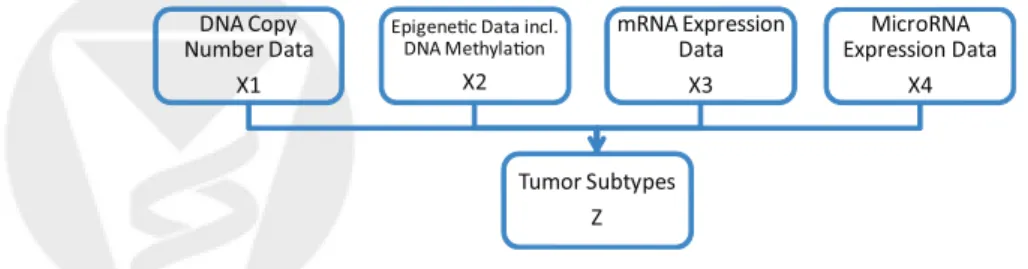
(denoted by X3, a matrix of dimensionp3×n), and so forth (Figure 1). The mathematical
form of the integrative model is
X1 = W1Z +ε1
X2 = W2Z +ε2
...
Xm = WmZ +εm,
(6)
where m is the number of genomic data types available for the same set of samples. We assume each data set is row centered and therefore intercept terms are not included in the models. In (6), Z is the latent component that connects the m-set of models, inducing
de-Tumor Subtypes Z DNA Copy
Number Data X1
Epigene!c Data incl. DNA Methyla!on X2 mRNA Expression Data X3 MicroRNA Expression Data X4
Figure 1: The integrative model. The concept is to formulate the tumor subtypes as the joint latent variable Z that needs to be simultaneously estimated from multiple genomic data types measured on the same set of tumors.
pendencies across the data types measured on the same set of tumors. On the other hand, the independent error terms(ε1,· · · , εm), in which each has mean zero and diagonal
covari-ance matrixΨi, represent the remaining variances unique to each data type after accounting
for the correlation across data types. Lastly, (W1,· · · ,Wm) denote the coefficient matrices.
In dimension reduction terms, they embed a simultaneous data projection mechanism that maximizes the correlation between data types.
To derive a likelihood-based solution of (6), we use a latent continuous parameterization that further assumes Z∗ ∼ N(0,I). The error term is ε
∼ N(0,Ψ), which has a diagonal
covariance matrix Ψ = diag(ψ1,· · · , ψP
ipi). The marginal distribution of the integrated
data matrix X= (X1,· · · ,Xm)′ is then multivariate normal with mean zero and covariance
matrix Σ = WW′ +Ψ, where W = (W
1,· · · ,Wm)′. The corresponding log-likelihood
function of the data is
ℓ(W,Σ) = −n 2 m X i=1 piln(2π) + ln det(Σ) +tr(Σ−1G) ! , (7)
where Gis the sample covariance matrix of the following form
G= G11 G12 · · · G1m G21 G22 · · · G2m ... ... . .. ... Gm1 Gm2 · · · Gmm . (8)
We employ the EM algorithm to obtain the maximum likelihood estimates of Wand Ψ. In the EM framework, we deal with the complete-data log-likelihood
ℓc(W,Ψ) =− n 2 nXm i=1 piln(2π) + ln det(Ψ) o − 12ntr((X−WZ∗)′Ψ−1(X−WZ∗)) +tr(Z∗′Z∗)o. (9)
This is a much more efficient approach than directly maximizing the marginal data likelihood in (7). It does not require explicit evaluation of the sample covariance matrices in (8), which would call for O(nPip2
i) operations and thus be computationally prohibitive.
Finally, the problem of p >> n is exacerbated in our model by the multiple high-dimensional data sets. A sparse solution toW is desirable. In the next Section, we derive a sparse solution to solve the iCluster model via penalizing the complete-data log-likelihood.
2.4
A Sparse Solution
We write the penalized complete data log-likelihood as
whereJλ(W) is a penalty term onWwith a nonnegative regularization parameterλ. Various
types of penalties can be employed. In this study, we use a lasso type (L1-norm) penalty
(Tibshirani , 1996) that takes the form
Jλ(W) = λ m X i=1 K−1 X k=1 pi X j=1 |wikj|. (11)
We derive the E-step and the M-step with respect to the penalized complete-data log-likelihood. The E-step involves computing the objective function
Qp(W,Ψ|W(t),Ψ(t)) = EZ∗|X,W(t)
,Ψ(t)[ℓc,p(W,Ψ)],
which is the expected value of the complete-data log-likelihood with respect to the distribu-tion of Z∗ given X under the current estimates (W(t),Ψ(t)). This involves computing the
following quantities given the current parameter estimates:
E[Z∗|X] =W′Σ−1X and E[Z∗Z∗′
|X] =I−W′Σ−1W+E[Z∗|X]E[Z∗|X]′. (12)
The E-step provides a simultaneous dimension reduction by mapping the original data ma-trices of joint dimensions (p1,· · · , pm)×n to a substantially reduced subspace represented
byZ∗ of dimension (K−1)×n.
The M-step is to update the parameter estimates by maximizing Qp subject tokwkk= 1
for all k. This leads to the following estimate of Ψ:
Ψ(t+1) = 1 ndiag
XX′−W(t)E[Z∗|X]X′ (13)
and the lasso estimate of W:
W(lassot+1) = sign(W(t+1)) |W(t+1)| −λ+, (14)
where W(t+1) = (XE[Z∗|X]′) (E[Z∗Z∗′
|X])−1. This is followed by a normalization step
wk/kwkk2 for all k, where kwkk2 denotes theL2 norm of the vector wk that takes the form qP
jw2jk. The algorithm iterates between the E-step and the M-step until convergence.
Once ˆE[Z∗|X] is obtained, a final step to recover the class indicator matrix is to invoke a
standard K-means on ˆE[Z∗|X]. We denote this solution as Zˆ
iCluster.
The lasso-type penalty results in sparse estimates ofW in which many of the coefficients are shrunken toward zero. The variance of the model is thus reduced, leading to better clustering performance though the bias-variance trade-off. The lasso also renders a variable selection mechanism owing to the L1 penalty that shrinks some coefficients to exactly zero. As a result, one can pinpoint which genes contribute to which subtype by finding the genes with non-zero loadings on the kth latent factor z
k. This will be demonstrated in the data
2.5
Model Selection Based on Cluster Separability
Let ˆB∗ = ˆE[Z∗|X]′Eˆ[Z∗|X] be ordered such that samples belonging to the same clusters
are adjacent. Then ˆB∗ has a diagonal block structure and can be used to assess cluster
separability. We standardize the elements of ˆB∗ to be b
ij/
p
biibjj for i = 1,· · · , n and
j = 1,· · ·, n, and impose a non-negative constraint by setting negative values to zero. Then perfect cluster separability (non-overlapping subclasses) would lead to an exact diagonal block matrix with diagonal blocks of ones for samples belonging to the same cluster and off-diagonal blocks of zeros for samples in different clusters. As cluster separability decreases, ˆB∗
increasingly deviates from the “perfect” diagonal block structure. We thus define a deviance measure d as the sum of absolute differences between Bˆ∗ and a “perfect” diagonal block
matrices of 1s and 0s. The proportion of deviance is defined as POD=d/n2 so that POD is
between 0 and 1. Small values of POD indicate strong cluster separability, and large values of POD indicate poor cluster separability. In the data examples, we show the utility of ˆB∗
matrix plots (we call them cluster separability plots) and associated the POD statistic for model selection, which includes estimating the number of clustersKand the lasso parameter
λ.
3
Results
3.1
Subtype Discovery in Breast Cancer
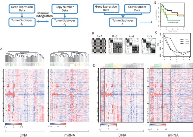
Pollack et al. (2002) studied 37 primary breast cancers and 4 breast cancer cell lines for DNA copy number and mRNA expression on the same cDNA microarrays that contain 6,691 genes. Figure 2A shows the pair of heatmaps displaying the alteration patterns in the DNA (left panel) and in the mRNA (right panel) on chromosome 17. Samples are arranged by separate hierarchical clustering output. Clearly the two dendrograms are substantially differ-ent. Although the leftmost clusters share members that carry the HER2/ERBB2 amplicon profile near 17q12, they are not identical. This is a problem inherent to separate clustering approaches that fail to account for the correlation between the two data sets. On the other hand, mixing breast tumors and cell line samples, the four cell line samples (BT474, T47D, MCF7, and SKBR3, indicated in red text) should be distinguished as a separate “subtype” from the rest of the tumor samples. This is clearly the case in the gene expression data, but it is not recapitulated in the DNA copy number data. This contrast shows the importance of capturing unique patterns specific to one data type.
Figure 2B-E show results of a unified set of cluster assignments from iCluster on the same data. Non-sparse (λ = 0) and sparse solutions (λ = 0.01 and 0.2) were generated. Figure 2B includes cluster separability plots described in Section 2.3 under the sparse solution given λ = 0.2. Clearly, K = 4 gives the best diagonal block structure. This is confirmed in Figure 2C where the 4-cluster sparse solution (λ = 0.2) minimized the POD statistic among a range of K and λ values. Figure 2D displays the heatmaps of the same data used
Gene Expression Data Tumor Subtypes Z Copy Number Data Gene Expression Data Tumor Subtypes Z1 Manual integra on Copy Number Data Tumor Subtypes Z2
NORWAY.10NORWAY.12NORWAY.57NORWAY.26NORWAY.101NORWAY.53STANFORD.
A
NORWAY.47STANFORD.
2
NORWAY.100NORWAY.17NORWAY.39NORWAY.104NORWAY.61NORWAY.65NORWAY.112STANFORD.14NORWAY.14 STANFORD.38STANFORD.17STANFORD.35
BT474SKBR3MCF7T47D
NORWAY.109NORWAY.111NORWAY.56NORWAY.41
STANFORD.23
NORWAY.7
STANFORD.16NORWAY.19NORWAY.15NORWAY.48NORWAY.11 STANFORD.24NORWAY.18NORWAY.27NORWAY.16NORWAY.102
NORWAY.53NORWAY.61STANFORD.2STANFORD.
A
BT474
NORWAY.26NORWAY.101NORWAY.57
SKBR3
NORWAY.47NORWAY.10NORWAY.11NORWAY.27NORWAY.109NORWAY.41NORWAY.65NORWAY.17NORWAY.18NORWAY.14NORWAY.16NORWAY.100STANFORD.35STANFORD.38NORWAY.111NORWAY.112NORWAY.102NORWAY.104STANFORD.17STANFORD.24
NORWAY.7NORWAY.39
T47D
NORWAY.12
MCF7
STANFORD.14NORWAY.48
STANFORD.23NORWAY.15NORWAY.19NORWAY.56
STANFORD.16
<−2 0 >2 <−1 0 >1
A
B
D
DNA mRNA DNA mRNA
1 7p 13 17p 12 17 p11 17q 11 17q 12 17q 21 1 7q2 2 17 q2 3 17 q2 4 17 q2 5 1 7p1 3 17 p1 2 1 7p1 1 1 7q1 1 1 7q1 2 1 7q 21 17q 22 17 q2 3 17 q24 17q 25 1 7p 13 1 7p 12 1 7p 11 17q 11 1 7q 12 17q 21 17q 22 1 7q 23 17 q2 4 17 q25 17p 13 17 p12 1 7p1 1 17q 11 17 q1 2 17q 21 1 7q 22 17 q2 3 17 q2 4 1 7q2 5 C BT474MCF7SKBR 3 T47DNORWAY.2 6 NORWAY.4 7 NORWAY.5 3 NORWAY.5 7 NORWAY.6 1 NORWAY.101STAN FORD. 2 STAN FORD. A NORWAY.1 5 NORWAY.1 9 NORWAY.4 1 NORWAY.4 8 NORWAY.5 6 NORWAY.109STAN FORD.16 STAN FORD.23 NORWAY.7NORWAY.1 0 NORWAY.1 1 NORWAY.1 2 NORWAY.1 4 NORWAY.1 6 NORWAY.1 7 NORWAY.1 8 NORWAY.2 7 NORWAY.3 9 NORWAY.6 5
NORWAY.100NORWAY.102NORWAY.104NORWAY.111NORWAY.112STAN
FORD.14 STAN FORD.17 STAN FORD.24 STAN FORD.35 STAN FORD.38 <−2 0 >2 BT474MCF7SKBR 3 T47DNORWAY.2 6 NORWAY.4 7 NORWAY.5 3 NORWAY.5 7 NORWAY.6 1 NORWAY.101STAN FORD. 2 STAN FORD. A NORWAY.1 5 NORWAY.1 9 NORWAY.4 1 NORWAY.4 8 NORWAY.5 6 NORWAY.109STAN FORD.16 STAN FORD.23 NORWAY.7NORWAY.1 0 NORWAY.1 1 NORWAY.1 2 NORWAY.1 4 NORWAY.1 6 NORWAY.1 7 NORWAY.1 8 NORWAY.2 7 NORWAY.3 9 NORWAY.6 5
NORWAY.100NORWAY.102NORWAY.104NORWAY.111NORWAY.112STAN
FORD.14 STAN FORD.17 STAN FORD.24 STAN FORD.35 STAN FORD.38 <−1 0 >1 E 0 20 40 60 80 0.0 0.2 0.4 0.6 0.8 1.0 Time in Months Surv ival Probability HER2 subtype K=2 K=3 K=4 K=5 2 3 4 5 6 0.15 0.25 0.35 0.45 K POD 2 3 4 5 6 0.15 0.25 0.35 0.45 2 3 4 5 6 0.15 0.25 0.35 0.45 λ=0 λ=0.01 λ=0.2
Figure 2: Results from separate clustering (left panel) and integrative clustering (right panel) using the Pollack data. A. Heatmaps of copy number (DNA) and gene expression (mRNA) on chromosome 17. Samples are arranged by separate hierarchical clustering on each data type. B. Cluster separability plots. C. Model selection based on POD measure. A 4-cluster sparse solution (λ = 0.2) was chosen. D. Heatmaps on the same data as in A with samples arranged by the integrated cluster assignment under the sparse iCluster model. E. Kaplan-Meier plots of the subclasses identified via the integrative clustering. The HER2/ERBB2
subtype showed poor survival.
in Figure 2A but with samples rearranged by their iCluster membership. In a completely automated fashion, the 4 cell lines were separated as cluster 1 (red). The HER2/ERBB2
subtype emerged as Cluster 2 (green) and showed coordinated amplification in the DNA and overexpression in the mRNA. This subtype was associated with poor survival as shown in Figure 2E. Cluster 3 was a potentially novel subtype derived only as a result of combining evidence across the two data sets. It represents a subset of tumors characterized by weak yet consistent amplifications toward the end of the q-arm of chromosome 17. Finally, cluster 4 did not show any distinct patterns, though a pattern may have emerged if there were additional data types. As mentioned in Section 2.4, the lasso-type penalty in the sparse iCluster solution renders variable selection as part of the outcome. Supplementary Table 1
lists the selected subset of genes associated with each of the subtypes.
3.2
Lung Cancer Subtypes Jointly Defined by Copy Number and
Gene Expression Data
We also analyzed a set of 91 lung adenocarcinomas from Memorial Sloan-Kettering Cancer Center, which is a subset of the samples in Chitale et al. (2009). The iCluster method was applied to perform integrative clustering on copy number and gene expression data. The copy number data were segmented using the CBS algorithm (Olshen et al., 2004;
Venkatra-man et al., 2007). The segment means were used as the input for integration to reduce the
noise level. Variance filtering based on gene expression was performed so as to focus on the most variable set of 2,782 genes.
Using chromosomes 8 and 12 as examples, we compared the iCluster results with those obtained by separate hierarchical clustering. Cluster 1 in Figure 3A is characterized by a broad region of 8p loss evident in the copy number heatmap and the corresponding under-expression in the under-expression heatmap. In contrast, this 8-p loss cluster is less well defined by separate clustering in Figure 3B. When annotated with somatic mutation status, this cluster shows significant enrichment of EGFR mutations (mutation panel on top of the heatmap). Specifically, 33% of the tumors in cluster 1 carry EGFRmutation, while 16%, 0%, and 18% of the tumors in cluster 2, 3, and 4 respectively, are EGFRmutant samples (Fisher’s exact test P=0.03). Another interesting observation made apparent by iCluster is that samples in cluster 4 show a similar but somewhat diluted pattern of copy number aberrations when compared to cluster 1. These samples may be related to cluster 1 but with lower tumor content, which may account for the 18% EGFR mutations in this cluster, the second highest among the four clusters. Chitale et al. (2009) describe the association between chromosome 8p loss and EGFR mutation in further details. When studying the genes within the broad region of 8p loss, they discovered a striking association between EGFR mutation and con-cordant DUSP4 deletion and underexpression. DUSP4 is known to be involved in negative feedback control of EGFR signaling. Notably, the sparse solutions consistently showed bet-ter clusbet-ter separability than the non-sparse solution as evidenced by Figure 3C.
Chromosome 12 is another interesting example. Cluster 2 in Figure 3D is characterized by the well-known 12q14-15 amplicon that includes oncogenes such as CDK4 and MDM2. Again, the sparse solution improves the cluster separability substantially from the non-sparse solution (Figure 3F). Interestingly, the non-sparse model selected only 24 DNA probes that contributed to the clustering, which is consistent with the observation that there are relatively few aberrations other than the small region of 12q gain in the DNA. Note, however, that genomic alteration patterns are often chromosome-specific (8p-loss and 12q-gain); They do not always occur in the same set of patients. Therefore, the results change when multiple chromosomes are combined (see Supplementary Figure 1).
A. Chr8 integrative clustering
B. Chr8 separate hierarchical clustering
D. Chr12 integrative clustering
E. Chr12 separate hierarchical clustering
DNA mRNA DUSP4.deleted PTEN TP53 ERBB2 PIK3CABRAF STK11 KRAS EGFR 2 3 4 5 6 7 8 0.15 0.25 0.35 0.45 K POD 2 3 4 5 6 7 8 0.15 0.25 0.35 0.45 2 3 4 5 6 7 8 0.15 0.25 0.35 0.45 λ=0 λ=0.05 λ=0.1 2 3 4 5 6 7 8 0.15 0.25 0.35 0.45 K POD 2 3 4 5 6 7 8 0.15 0.25 0.35 0.45 2 3 4 5 6 7 8 0.15 0.25 0.35 0.45 λ=0 λ=0.05 λ=0.1 C. Model selection (chr8) F. Model selection (chr12) DUSP4.deleted PTENTP53 ERBB2 PIK3CABRAF STK11 KRAS EGFR DUSP4.deleted PTEN TP53 ERBB2 PIK3CABRAF STK11 KRAS EGFR DUSP4.deletedPTEN TP53 ERBB2 PIK3CABRAF STK11 KRAS EGFR
Figure 3: Lung cancer subtypes for chromosome 8 and 12. A. Heatmap of DNA copy number (left) and mRNA expression (right) on chromosome 8. Columns are tumors arranged by the 3 subclasses obtained by iCluster. Rows are genes ordered by genomic position. On top of the heatmaps are gray-dot panels indicating mutation status of several well-known lung cancer genes. B. Separate hierarchical clustering of the same data on chromosome 8 used in A. C. Model selection based on the POD measure. A 4-cluster sparse solution (λ = 0.05) was chosen that selected 301 mRNA probes and 126 DNA probes from a total of 642 probes. D. iCluster output on chromosome 12. Tumor samples are arranged by the 6 subclasses obtained by iCluster. E. Separate hierarchical clustering of the same data on chromosome 12 used in D. F. Model selection based on the POD statistic. A 6-cluster sparse solution (λ = 0.1) was chosen that selected 408 mRNA probes and 24 DNA probes from a total of 1038 probes.
4
Discussion
Despite the ever-increasing volume of multiple genomic platform (MGP) data resulting from the Cancer Genome Atlas project and other studies, there is a shortage of effective integra-tive methods. Researchers often resort to heuristic approaches where “manual integration” is performed after separate analysis of individual data types, and it is unlikely two inves-tigators would perform manual integration in the same manner. Manual integration may require a considerable amount of prior knowledge about the underlying disease. In contrast,
the iCluster method developed here generates a single integrated cluster assignment based on simultaneous inference from multiple data types. In both the breast and lung cancer data examples, we have shown that iCluster aligns concordant DNA copy number aberrations and gene expression changes. In some cases, potentially novel subclasses are revealed only by combining weak yet consistent evidence across data types.
In this study, we applied iCluster to integrate copy number and gene expression data. The joint latent variable model is completely scalable to include additional data types. Next-generation sequencing is emerging as an appealing alternative to microarrays for inferring RNA expression levels (mRNA-Seq), DNA-protein interactions (ChIP-Seq), DNA methyla-tion, and so on. Although we focus here on array data, our integrative framework could be generalized to next-gen sequencing data after proper modifications of the error terms to model count data based on mapped reads.
Acknowledgments
We thank Drs. Colin Begg, Glenn Heller, and Richard Olshen for helpful comments. We thank the reviewers for their constructive comments, which we used to improve the manuscript. This research is supported in part by Cancer Center Support Grant P30 CA008748.
References
Alter, O., Brown, P.O. and Botstein, D. (2000). Singular value decomposition for genome-wide expression data processing and modeling.
Proceedings of the National Academy of Sciences,97, 10101–10106.
Brunet, J.P., Tamayo, P., Golub, T.R. and Mesirov, J.P. (2004). Metagenes and molecular pattern discovery using matrix factorization.
Proceedings of the National Academy of Sciences,101, 4164–4169.
Olshen A.B., Venkatraman E.S., Lucito R., and Wigler M. (2004). Circular binary segmentation for the analysis of array-based DNA copy number data.Biostatistics,5, 557–72.
Venkatraman E.S. and Olshen A.B. (2007). A faster circular binary segmentation algorithm for the analysis of array CGH data.
Bioinformatics,23, 657–63.
Chitale D., Gong Y., Taylor B.S., Broderick S., Brennan C., Somwar R., Golas B., Wang L., Motoi N., Szoke J., Reinersman J.M., Major J., Sander C., Seshan E.V., Zakowski M.F., Rusch V., Pao W., Gerald W., and Ladanyi M. (2009). An integrated genomic analysis of lung cancer reveals loss ofDUSP4inEGFR-mutant tumors.Oncogene,28, 2773–83.
Dempster, A.P., Laird, N.M. and Rubin, D.B. (1977). Maximum Likelihood from Incomplete Data via the EM Algorithm.Journal of the Royal Statistical Society: Series B (Statistical Methodology),39, 1–38.
Ding, C.H.Q. and He, X. (2004). K-means clustering via principal component analysis. InICML, vol. 69 of ACM International Conference Proceeding Series, ACM.
Holter, N.S., Mitra, M., Maritan, A.et al.(2000). Fundamental patterns underlying gene expression profiles: Simplicity from complexity.
Proceedings of the National Academy of Sciences,97, 8409–8414.
Hyman, E., Kauraniemi, P., Hautaniemi, S.et al.(2002). Impact of DNA amplification on gene expression patterns in breast cancer.
Kool, M., Koster, J., Bunt, J.et al.(2008). Integrated genomics identifies five medulloblastoma subtypes with distinct genetic profiles, pathway signatures and clinicopathological features.PLoS ONE,3, e3088–e2102.
Lee, H., Kong, S.W. and Park, P.J. (2008). Integrative analysis reveals the direct and indirect interactions between DNA copy number aberrations and gene expression changes.Bioinformatics,24, 889–896.
Lewis, B.P., Burge, C.B. and Bartel, D.P. (2005). Conserved seed pairing, often flanked by adenosines, indicates that thousands of human genes are microrna targets.Cell,120, 15–20.
Pollack, J.R., Sørlie, T., Perou, C.M.et al.(2002). Microarray analysis reveals a major direct role of DNA copy number alteration in the transcriptional program of human breast tumors.Proceedings of the National Academy of Sciences,99, 12963–12968. Qin, L.X. (2008). An Integrative Analysis of microRNA and mRNA Expression - A Case Study.Cancer Informatics,6, 369–379. TCGA (2008). Comprehensive genomic characterization defines human glioblastoma genes and core pathways.Nature,455, 1061–1068. Tipping, M.E. and Bishop, C.M. (1999). Probabilistic principal component analysis.Journal of the Royal Statistical Society: Series
B (Statistical Methodology),61, 611–622.
Zha, H., He, X., Ding, C.H.Q., Gu, M. and Simon, H.D. (2001). Spectral Relaxation for K-means Clustering. InNIPS, 1057–1064, MIT Press.
Tibshirani, R. (1996). Regression shrinkage and selection via the lasso. InJournal of the Royal Statistical Society: Series B (Statistical Methodology),58, 267–288.
Tibshirani, R., Walther, G. and Hastie, T. (2000). Estimating the number of clusters in a dataset via the gap statistic.Journal of the Royal Statistical Society: Series B (Statistical Methodology),63, 411–423.
Rand, W.M. (1971). Objective criteria for the evaluation of clustering method.Journal of the American Statistical Association,66, 846–885.
Dudoit, S. and Fridlyand, J. (2002). A prediction-based resampling method for estimating the number of clusters in a dataset.Genome Biology,3, 1–21.
Fallah, S., Tritchler, D. and Beyene, J. (2008). Estimating number of clusters based on a general similarity matrix with application to microarray data.Statistical Applications in Genetics and Molecular Biology,7, Art. 24.