SFB 649 Discussion Paper 2007-027
Long Memory Persistence
in the Factor of Implied
Volatility Dynamics
Wolfgang Härdle*
Julius Mungo*
* Humboldt-Universität zu Berlin, Germany
This research was supported by the Deutsche
Forschungsgemeinschaft through the SFB 649 "Economic Risk". http://sfb649.wiwi.hu-berlin.de ISSN 1860-5664 SFB 649, Humboldt-Universität zu Berlin
S
FB
6
4
9
E
C
O
N
O
M
I
C
R
I
S
K
B
E
R
L
I
N
Long Memory Persistence in the Factor of
Implied Volatility Dynamics
Wolfgang Karl H¨
ardle
1, Julius Mungo
21CASE – Center for Applied Statistics and Economics, Humboldt-Universit¨at zu Berlin, Spandauer Straße 1, 10178 Berlin, Germany
2CASE – Center for Applied Statistics and Economics, Humboldt-Universit¨at zu Berlin, Spandauer Straße 1, 10178 Berlin, Germany; e-mail: [email protected]; phone: +49(0)30 2093-5654
Abstract
The volatility implied by observed market prices as a function of the strike
and time to maturity form an Implied Volatility Surface (IV S). Practical
applications require reducing the dimension and characterize its dynamics through a small number of factors. Such dimension reduction is summarized
by a Dynamic Semiparametric Factor Model (DSF M) that characterizes the
IV S itself and their movements across time by a multivariate time series of
factor loadings. This paper focuses on investigating long range dependence in the factor loadings series. Our result reveals that shocks to volatility per-sist for a very long time, affecting significantly stock prices. For appropriate representation of the series dynamics and the possibility of improved fore-casting, we model the long memory in levels and absolute returns using the class of fractional integrated volatility models that provide flexible structure to capture the slow decaying autocorrelation function reasonably well.
JEL classification: C14, C32, C52, C53, G12
Keywords: Implied Volatility, Dynamic Semiparametric Factor Modeling, Long Memory, Fractional Integrated Volatility Models
Acknowledgement: This research was supported by the Deutsche Forschungs-gemeinschaft through the SFB 649 ‘Economic Risk’
1
Introduction
As a measure of the standard deviation of the daily range of price move-ments, volatility is an important determinant of the riskiness of an asset, a crucial parameter in derivative pricing such as options. Findings across several asset markets have reported high persistence of volatility shocks and that over sufficiently long periods of time, volatility is typically stationary with ”mean reverting” behavior, Bollerslev and Jubinski (1999). Such series are characterized by distinct but nonperiodic cyclical patterns and their be-havior is such that current values are not only influenced by immediate past values but values from previous time periods, allowing for persistence or long memory. Long memory describes the correlation structure of a series at long lags.
It is well known that the volatility implied by observed option prices as a function of the strike and time to maturity form an Implied Volatility
Sur-face (IV S). For each day the IV S forms a high dimensional object that has
unknown stochastic behavior that needs to be analyzed. For practical appli-cations such as in risk management, it is desirable to reduce the dimension of this object and characterize its dynamics through a small number of factors. Such dimension reduction may be summarized by a Dynamic
Semiparamet-ric Factor Models (DSF M) that characterize theIV S and their movements
across time by a multivariate time series of factor loadings, Borak et al. (2005), Fengler et al. (2007) and Borak et al. (2007).
TheDSF Ms approximate the implied volatility surface by regressing log-implied volatility on a two-dimensional covariate containing moneyness and
time-to-maturity. To introduce this model, denote by Yt,j = log{σˆt,j(κ, τ)},
the log-implied volatility where t = 1, . . . , I is an index of time, in this case
the number of the day, and j = 1, . . . , Jt is the number of IV observations
on day t. Let Xt,j = (κt,j, τt,j) be a two-dimensional covariate where κt,j is a
moneyness matrix andτt,j denotes time-to-maturity. Moneyness is defined as
κt,j = Kt,j
Ft,j where Kt,j is a strike andFt,j =Ste
(rt,j,τt,j) the underlying futures
price belonging to the option trade (t, j). The model is expressed as:
Yt,j = K
X
k=0
zt,kmk(Xt,j) +εt,j (1)
wherezt,0 = 1,mkare smooth basis functions (k = 0, . . . , K) andzt,kare time
dependent weights or factor loadings. The IV S is assumed to be a weighted
the stochastic behavior of the factor loadings, zt,k. Approximations of the
factor loadings are obtained by fitting model (1) to the implied volatility
ob-servations and the functionsmkare estimated by orthogonal series estimators
so that they have zero correlations among each other, Borak et al. (2005).
The factor loadings zt = (zt,1, . . . , zt,K)> forms an unobserved multivariate
time series.
The estimates zbt,k and mbk are obtained in (1) as minimizers of the
fol-lowing least squares criterion:
I X t=1 Jt X j=1 Z ( Yt,j− K X k=0 b zt,kmbk )2 Kh(u−Xt,j)du, (2)
where Kh denotes a two-dimension kernel function, chosen as a product of
one-dimensional kernels Kh(u) = kh1(u1)× kh2(u2), where h = (h1, h2)
>
are bandwidths and kh(v) = k(h−1v)/his a one-dimensional kernel function.
The minimization procedure is iterative, searching through all functionsmbk:
R2 −→ R (k = 0, ..., K) and time series zbtk ∈ R (t = 1, ..., I;k = 1, ..., K).
The estimation procedure can be seen as a combination of functional princi-pal component analysis, nonparametric curve estimation and backfitting for
additive models. The DSF M therefore simultaneously estimate the factor
functions and fits the surface.
This paper applies theDSF M on the GermanDAX index market from
04.01.1999 to 25.02.2003. Figure 1 displays the implied volatility surface
from the DSF M fit for the DAX-Option on 2 May 2000, with moneyness
between 0.8 and 1.12 and time to maturity between 0 and 0.5 years. Figure
2 shows three volatility-driving factors that could be interpreted in terms of
level, slope and curvature factor. z1 governs movements in the general level,
z2 is largely associated with changes in the slope and z3 is closely related to
dynamic changes in the curvature of the IVS.
The aim of this paper is to investigate dependence in the factor loadings of implied volatility strings because information on persistence can guide the search for economic explanation of the movements in asset returns as well as in risk management applications. Several research involving the autocor-relation functions of various volatility measures (squared, log-squared and absolute returns) have reported decay at a very slow mean-reverting hyper-bolic rate, Ding et al. (1993), Bollerslev and Wright (2000) and Sibbertsen (2004). Our analysis follow this line of research on long range dependence investigation and modeling.
0.14 0.23 0.32 0.41 0.50 0.80 0.88 0.96 1.04 1.12 -1.47 -1.31 -1.16 -1.00 -0.85 Time to maturity
log implied volatility
moneyness
Figure 1: Implied volatility surface from DSFM fit for the DAX-Option on
2 May 2000, with moneyness between 0.8 and 1.12 and time to maturity
between 0 and 0.5 years.
1999 2000 2001 2002 2003
0.5
1
1.5
First loading series: Z1
1999 2000 2001 2002 2003 -0.3 -0.2 -0.1 0 0.1
Second loading series: Z2
1999 2000 2001 2002 2003 -10 -5 0 5 10
Third loading series: Z3
Figure 1: Factor Loading Time Series from Dynamic Semiparametric Model for Implied
Volatility String Dynamics.
Figure 2:Factor Loading Time Series from Dynamic Semiparametric Model for Implied Volatil-ity String Dynamics (left column).
14
Figure 2: Time series plots in levels of three loading series from a DSFM fit
for the DAX-Option analyzed from 04.01.1999−25.02.2003
First, we consider model independent tests for stationarity, I(0) against
fractional alternatives I(d). We apply the rescaled variance test (V /S) of
Giraitis et al. (1999) that uses the heteroscedastic and autocorrelation
con-sistent (HAC) estimator of the variance, Newey and West (1987) for
nor-malization and the semiparametric (LobRob) test of Lobato and Robinson
(1998), that does not depend on a specific parametric form of the spectrum in the neighborhood of the zero frequency. We also apply the log-periodogram
regression estimator (GP H) of Geweke and Porter-Hudak (1983) and the
Gaussian Semiparametric estimator (GSP) of Robinson (1995a) in
estimat-ing the degree of long memory in the factor loadestimat-ings series. Results are indicative of long-range dependence in the factor loadings series in levels and
absolute returns. The first factor, z1 can be interpreted as highly
persis-tent and influences all options similarly, irrespective of maturity. The second
factor z2 gradually diminishes for longer maturities and the third factor z3
governs large volatility changes in relatively short maturities.
Second, for appropriate representation of the series dynamics and the possibility of improved forecasting, we model long memory in volatility using the ARF IM A, F IGARCH and HY GARCH models. These models pro-vide flexible structure that captures slow decaying autocorrelation reasonably well. In comparison, models in absolute returns have better performance, confirming the findings of Ding et al. (1993), that absolute returns are most appropriate indicator to represent the long memory volatility processes. Our results imply that shocks to the volatility will persist for long time, affecting
the DAX stock prices significantly.
Such dependence or persistence will have importance economic conse-quences for short-term trading and long range investment strategies. Better option pricing may results from models that price and hedge derivative secu-rities when there is prior information on long-memory volatility in terms of expectation on the potential level of volatility and the rate at which volatil-ity changes. In the presence of long memory, Granger and Joyeux (1980), Geweke and Porter-Hudak (1983) have shown the possibility for improved price forecasting performance within a linear time series framework than with traditional procedures. Option pricing have also been shown to be sig-nificantly different when standard models are applied as compared to models allowing for long memory.
By applying the GARCH, EGARCH, F IEGARCH and IEGARCH
models, Bollerslev and Mikkelsen (1996) have shown that the price of an
option increases with the degree of integration. This means that GARCH
for the IGARCH model. For long memory alternative, Herzberg and
Sib-bertsen (2004) have shown that prices for the F IGARCH,HY GARCH are
inbetween the GARCH and IGARCH prices. In addition to documented
studies of the economic implications of long memory, Cheung and Lai (1995), Wilson and Okunev (1999), revealed that portfolio diversification decisions in the case of strategic asset allocation may become extremely sensitive to the investment horizon. There may be diversification benefits in the short and medium term, but not if the assets are held together over the long term if long memory is present. e.g., in a market that exhibits antipersistence, asset prices tend to reverse its trend in the short term thus creating short-term trading opportunities. In addition Mandelbrot (1971) has shown that in the presence of long memory the arrival of new market information cannot be fully arbitraged away. It is also known that the possibility of speculative profits as a result of superior long-range dependence model forecast would cast doubt on the basic tenets of market efficiency.
Motivated by evidence of long range dependence in the factor loadings levels and absolute returns, we perform estimation and prediction using the
ARF IM A,F IGARCH andHY GARCH models that are known to provide flexible structure to capture slow decaying autocorrelation reasonably well
than with traditional ARM A procedures.
The rest of our work is structured as follows. Section 2, introduces
fractional integration and Long-memory processes. Here we examine some methodology for testing and estimating long range dependence that we apply in our analysis. Section 3 introduces the structure of the class of models we apply to analyze the long memory in the factor loading series. In section 4 we report and discuss our results for the series in levels and absolute returns. A summary of our analysis results and conclusions is given in section 5.
2
Fractional integration and long-memory
The framework of fractional integration yields convenient modeling of long range dependence, Granger and Joyeux (1980), Baillie (1996). A time series
process zt is integrated of order d, I(d) if
(1−L)dzt =εt (3)
where εt ∈ I(0) and L is the lag operator (Lzt = zt−1). The non-integer
parameter d is the difference parameter and (1−L)d is the fractional filter
defined by its binomial expansion (1−L)d=P∞
j=0
Γ(j−d) Γ(−d)Γ(j+1)L
R∞
0 t
z−1e−tdt is the gamma function. The autocorrelation function of such a
series is given by
ρk =
Γ(1−d)Γ(k+d)
Γ(d)Γ(k+ 1−d) ∼Ck
2d−1 (4)
for d in the range of (0,0.5), where C is a strictly positive constant. In
such case zt is said to exhibit long memory. For 0 < d < 0.5, the series
is stationary. For d = 0, the series is an I(0) process and said to have no
long-memory. For 0.5 < d < 1 the process is mean reverting as there is
no long run impact of an innovation to future values of the process. In the
case where 0 < d <1, not only the immediate past value of zt influence the
current value, but also values from previous time periods as well. The sum over the autocorrelation does not converge, so that it is a suitable model for long memory, Granger and Joyeux (1980).
2.1
Tests and estimators of long memory processes
We consider two model independent tests for stationarity, I(0) against
frac-tional alternatives I(d). The tests include the rescaled variance test (V /S)
of Giraitis et al. (1999) that uses the heteroscedastic and autocorrelation
consistent (HAC) estimator of the variance, Newey and West (1987) for
nor-malization and the semiparametric (LobRob) test of Lobato and Robinson
(1998), that does not depend on a specific parametric form of the spectrum in the neighborhood of the zero frequency.
The Rescaled Variance testis applied by centering theKP SSstatistic
based on the partial sum of the deviations from the mean:
V /S(q) = 1 T2σˆ2 T(q) T X k=1 ( k X j=1 (zj−zT) )2 − 1 T ( T X k=1 k X j=1 (zj−zT) )2 (5)
where Sk = Pkj=1(zj − zT) are the partial sums of the observations and
ˆ σ2 T(q) = ˆγ0+ 2 Pq j=1
1− 1+jqγˆj,is the heteroscedastic and autocorrelation
consistent (HAC) estimator of the variance, (q < T). γˆ0 is the variance
of the process, and the sequence {γˆj}qj=1 denotes the autocovariances of the
process up to the order q. Giraitis, Kokoszka and Leipus (2000) have shown
that this statistic can detect long range dependence in the volatility for the
The Semiparametric test is based on the approximation of the spec-trum of a long memory process. This test allows to discriminate between
d > 0 and d < 0. In the univariate case the test statistic for I(0) against
I(d) is given by tLobRob = p (m)Cb1 b C0 (6)
with Cbk = m1 Pjm=1ζjkI(λj) and ζj = log(j)− m1 Pmi=1log(i), where
I(λ) = 2πT1 PT t=1zte itλ 2
, (i = √−1) is the estimated periodogram. λj =
2πj
T , j = 1, . . . , m << [T /2] is a degenerate band of Fourier frequencies
with bandwidth parameter m. Under the null hypothesis the test statistic is
asymptotically normally distributed. If the statistic is in the lower fractile of the standardized normal distribution, the series exhibit long-memory whilst if in the upper fractile of that distribution, the series is antipersistent.
To estimate the memory parameter d, we apply two frequently used
es-timators, the log-periodogram regression estimator (GP H) of Geweke and
Porter-Hudak (1983) and the Gaussian Semiparametric estimator (GSP) of
Robinson (1995a).
The log-periodogram regression estimator is based on the
peri-odogram of a time series zt, (t= 1, . . . , T) defined by
I(λj) = 1 2πT T X t=1 zte−iλt 2 (7)
where λj = 2Tπj, j = 1, . . . , m (m is a positive integer). The memory
para-meter d is estimated from a linear regression of the logI(λj) on a constant
and the variable Xj = log
4 sin2(λj/2) : b dGP H =− Pm j=1(Xj−X¯) log{I(λj)} 2Pm j=1(Xj−X¯) (8)
We consider only harmonic frequencies λj = 2Tπj, (thejth Fourier frequency)
with j ∈ (l, m], where l is a trimming parameter discarding the lowest
fre-quencies and m is a bandwidth parameter. The cut-off parameter ensures
robustness of the estimator. For the Gaussian case with d ∈ (−0.5,0.5),
the estimator is consistent and asymptotically normal with standard error of
π/√24m, Robinson (1995b).
Validity of the GP H estimator for an enlarged interval has been
[0.5,0.75), where the time series is nonstationary, asymptotic Normality and
consistency is preserved as in the original interval (−0.5,0.5), while for values
ofdin the interval [0.75,1) the estimator is still consistent. Deo and Hurvich
(2001) have shown that this estimator is also valid for some non-Gaussian time series.
The Gaussian Semiparametric estimator is based on the
approxi-mation, limλi→0+f(λi) = Cλ
−2d
i of a long memory process in the Whittle
approximate maximum likelihood estimator, LW(θ). For m∗ = [T2], an
ap-proximation to the Gaussian likelihood, Beran (1994) is given by
LW(θ) =− 1 2π m∗ X j=1 logfθ(λj) + IT(λj) fθ(λj) (9)
for a given parametric spectral density fθ(λ). Estimating dis by solving the
minimization, arg min C,d L(C, d) = 1 m m X j=1 ( log(Cλ−j2d) + I(λj) Cλ−j2d )
where I(λj) is the periodogram evaluated for a degenerated range of m
har-monic frequencies λj = 2Tπj, j = 1, . . . , m << [T2], where [.] represents the
integer part operator, bounded by the bandwidth parameter m, which
in-creases with the sample size T but more slowly. This bandwidth m must
satisfy m1 + mT → 0 as T → ∞. If m = [T2], this estimator is a Gaussian
estimator for the parametric model f(λ) = Cλ−2d.
An estimator ford is given by
ˆ dGSP = arg min d ( log 1 m m X j=1 I(λj) Cλ−j2d ! − 2d m m X j=1 log(λj) ) . (10)
Robinson (1995a) showed that √m( ˆdGSP −d)
d
→ N(0,1/4) and is valid in
the presence of some form of conditional heteroscedasticity, Robinson and Henry (1999). In general, Phillips and Shimotsu (2004) have shown that the ranges of consistency and asymptotic normality for the model type in (3) are
thesame as those of the GP H estimator.
3
Long Memory Models
Several studies have dealt with models that provide useful ways of analyzing the relationships between the conditional mean and variance of a process
ex-hibiting long memory and slow decay in its levels. In our analysis we consider
an autoregressive fractional integrated moving average (ARF IM A) process
model, Granger and Joyeux (1980), Hosking (1981), the (F IGARCH),
Bail-lie et al. (1996), a combination of fractional integrated process for the mean
with regular GARCH process for conditional variance and the HYperbolic
GARCH, (HY GARCH) of Davidson (2004).
The ARFIMA(p,d,q)model represented as
Φ(L)(1−L)d(zt−µ) = Θ(L)εt (11)
where εt ∼ i.i.d(0, σε2) extends the integration order of the conventional
ARM A model to a non-integer value between 0 and 1. Φ(L) = 1−φ1L− φ2L2− · · · −φpLp and Θ(L) = 1 +θ1L+θ2L2+· · ·+θqLq are the
autoregres-sive and moving average polynomials in the lag operator L respectively. d
is the long memory parameter and (1−L)d is the fractional difference filter
as defined in equation 3. The ARF IM A process displays persistence for
0< d <0.5 and anti-persistence for −0.5< d <0. For |d|>0.5, the process is non-stationary as it has finite variance.
In our application, the values forpandqare chosen such that the ordered
pair (p, q) minimizes theAIC criterion. We estimate the model parameters
µ,φ,θ and dby maximum likelihood approach of Doornik and Ooms (2004)
that allows for (break-) regressors in the mean and structural changes in the variance, and by non-linear least squares estimation method of Beran (1994)
that is asymptotically efficient in the presence of GARCH errors.
The FIGARCH(p,δ,q) model of Baillie et al. (1996) given as
Φ(L)(1−L)dεt2 =ω+ Θ(L)νt (12)
where νt = ε2t −σ2t combine the fractional integrated process for the mean
with regular GARCH process for the conditional variance. The conditional
variance can be represented as
σ2t = ω 1−θ(L) + 1− φ(L)(1−L) δ 1−θ(L) ε2t (13)
with 0 ≤δ≤1. Theδ inF IGARCH does not have the same interpretation
of persistence as din ARF IM A. The fractional differencing operator in the
ARF IM A model applies to the constant term in the mean equation while inF IGARCH it does not apply toω in the variance equation. We base our
analyis on the F IGARCH parametrization proposed by Chung (1999),
where σ2 is the unconditional variance of εt. The conditional variance is formulated as σt2 =σ2+ 1− φ(L)(1−L) δ 1−θ(L) (ε2t −σ2) (15)
For p = q = 1, Chung (1999) shows that σ2 > 0 and 0 ≤ φ
1 ≤ θ1 ≤ 1
is a sufficient condition for positive σ2
t. When δ = 0 or 1, the F IGARCH
model nests the GARCH(p, q) and IGARCH processes respectively. The
IGARCH model is a short memory process having no variance and while the F IGARCH has shortest memory with δ > 0 closest to 1. If δ > 0 the F IGARCH is a non-stationary long memory process, otherwise is a stationary long memory process, Laurent and Peters (2002). The fractional difference filter is defied by,
(1−L)δ = ∞ X j=0 Γ(δ+ 1) Γ(j + 1)Γ(δ−j+ 1)L j (16) = 1−δL− 1 2δ(1−δ)L 2− 1 6δ(1−δ)(2−δ)L 3−. . . (17) = 1− ∞ X j=1 Cj(δ)Lj (18)
such thatC1(δ) = δ,C2(δ) = 12δ(1−δ), etc. By construction,P∞
j=1Cj(δ) = 1
for any δ, belonging to same class type models as the IGARCH.
The hyperbolic GARCH model, HYGARCH(p,α,d,q) of Davidson
(2004) extends the conditional variance of the F IGARCH(p, δ, q) model by
introducing weights to the difference operator in equation 12 such that (1−
L)d=
(1−α) +α(1−L)d
. The parametrization ofHY GARCH(p, α, d, q)
models is given by σ2t = ω 1−θ(L) + " 1− φ(L) 1 +α(1−L)d 1−θ(L) # ε2t (19)
where α are weights to (1 − L)d. The parameters α and d are assumed
positive. The HY GARCH(p, α, d, q) nest GARCH models (for α = 0),
IGARCH (for α=d= 1) and F IGARCH (for α= 1 or logα= 0). When
4
Empirical Analysis
The factor loadings series data are obtained from DSFM for implied
volatil-ity on the GermanDAX index market from January 1999 to February 2003
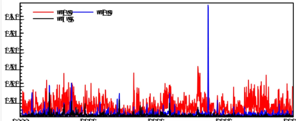
(data available at, http://sfb649.wiwi.hu-berlin.de/fedc). Table 1 presents descriptive statistics. Plots of sample autocorrelation functions, spectrum and periodogram (on log-log plane) are shown in Figure 3. The autocorre-lation are positive and decay hyperbolically to zero as the lag increases. A linear relationship in the periodogram on log-log plane indicates the presence of self-similarities, the fluctuations in a power-law fashion. Figure 4 shows time series plots in absolute returns of three factor loadings series.
Since unit root tests are known to perform relatively poorly in
distinguish-ing betweenI(1) and theI(d) alternatives ford <1, Diebold and Rudebusch
(1991), we apply model independent tests, V /S and LobRob forI(0) against
I(d) alternatives. With no data driven guideline for the choice of truncation
lags m, we use different values (m = 2,3,5,7,10,20,50) in theV /S test and
(m= 30,50,150,200,300) in LobRob test.
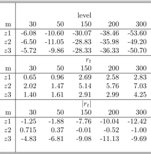
Results in Tables 2 and 3 for the V /S and LobRob tests respectively
in-dicate long-range dependence in all three factor loadings levels. For absolute
returns, the tests indicate long momory in |z1| and|z3|while antipersistence
could not be rejected in |z2|. Both tests results reject long memory for all
factor loadings returns.
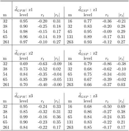
Table 4 shows the ˆdGP H and ˆdGSP estimates of d for the series in levels,
returns and absolute returns. To evaluate the sensitivity of results for the ˆ
dGP H estimator, we report estimates of d for bandwidth m = Tα where
α = 0.5,0.525,0.575,0.60,0.80 and T = 1052 is the sample size. For the
GSP estimator the bandwidth is chosen such thatm= [T4],[T8],[16T ],[32T],[64T].
Results for series in levels show 0.5 ≤ d < 1; for the return series most
estimates from ˆdGP H and ˆdGSP are in −0.5≤d < 0 while estimates of d for
the absolute returns are within 0≤d <0.5.
To guarantee that the long memory diagnosis is not a consequence of
occasional or structural break such as the 11th September, 2001 terrorist
at-tack on the World Trade Center, we use subsamples of the data to examine whether long run dependencies can be uncovered, Anderson and Bollerslev
(1998). This approach is possible given that the value of d is not affected
by temporal aggregation, Bollerslev and Wright (2000). Results, not pre-sented here indicate long memory for short span of the data in levels and absolute returns. This therefore suggest that long memory is an inherent
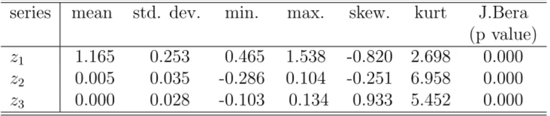
series mean std. dev. min. max. skew. kurt J.Bera (p value)
z1 1.165 0.253 0.465 1.538 -0.820 2.698 0.000
z2 0.005 0.035 -0.286 0.104 -0.251 6.958 0.000
z3 0.000 0.028 -0.103 0.134 0.933 5.452 0.000
Table 1: Summary statistics for factor loadings times series on the German
DAX index market from January 1999 to February 2003, a sample of 1039
observations. 0 50 100 150 200 250 300 lag 0 0.5 1 acf ACF-z1 0 0.1 0.2 0.3 0.4 0.5 frequency 0 0.1 0.2 0.3 0.4 density Spectrum-z1 -4 -3 -2 -1 0 1 X -5 0 5 Y log-log Periodogram z1 0 50 100 150 200 250 300 lag 0 0.5 1 acf ACF-z2 0 0.1 0.2 0.3 0.4 0.5 frequency 0 2 4 6 density*E-3 Spectrum-z2 -4 -3 -2 -1 0 1 X -5 0 5 Y log-log Periodogram z2 0 50 100 150 200 250 300 lag 0 0.5 1 acf ACF-z3 0 0.1 0.2 0.3 0.4 0.5 frequency 0 1 2 3 4 5 density*E-3 Spectrum-z3 -4 -3 -2 -1 0 1 X -5 0 5 Y log-log Periodogram z3
Figure 3: Plots of sample autocorrelation functions (lag length 300), spectrum
and periodogram (in the log-log plane) of the factor loadings series.
characteristics of the factor loading series.
To summarize, our analysis suggest long-range dependence in loading
levels as well as in absolute returns forz1 andz3. In general no long memory
in returns was detected and evidence of antipersistence in the absolute returns
forz2 could not be ruled out. We therefore interpret that there is quite some
correlation structure in the loadings in levels as well as in absolute returns. This implies some degree of persistence and the expectation of a slow decay in impulse responses. We also observe that the long range dependence is different for each factor loading such that it could be interpreted in terms of a long term, middle long term and short term impact on the dynamics
of IV S. The first factor loading, z1 is highly persistent and influences all
options similarly, irrespective of maturity. The impact of the second factor
loading, z2 gradually diminishes for longer maturities, while the third factor
Data Plot 02/14/07 20:21:23 Page: 1 of 1 1999 2000 2001 2002 2003 0.05 0.10 0.15 0.20 0.25 0.30 |z1| |z3| |z2|
Figure 4: Time series plots of the three factor loading series in absolute
returns from 04.01.1999−25.02.2003 level m 2 3 5 7 10 20 50 z1 4.63 3.29 2.22 1.68 1.24 0.68 0.32 z2 3.77 2.89 1.99 1.54 1.15 0.65 0.31 z3 3.54 2.68 1.82 1.38 1.02 0.57 0.27 rt m 2 3 5 7 10 20 50 z1 0.02 0.02 0.03 0.03 0.04 0.05 0.06 z2 0.00 0.01 0.01 0.01 0.01 0.02 0.03 z3 0.01 0.01 0.02 0.02 0.03 0.03 0.04 |rt| m 2 3 5 7 10 20 50 z1 0.24 0.21 0.19 0.15 0.13 0.09 0.07 z2 0.05 0.05 0.05 0.04 0.05 0.04 0.04 z3 0.84 0.78 0.72 0.64 0.56 0.44 0.28
Table 2: The rescaled variance V /S test for I(0) against I(d) for series in
levels, return (rt) and absolute return (|rt|). q is the truncation lag. If the
evaluated statistics are over the critical value, 0.1869 for I(0), we fail to reject the alternative hypothesis that the series display long memory.
level m 30 50 150 200 300 z1 -6.08 -10.60 -30.07 -38.46 -53.60 z2 -6.50 -11.05 -28.83 -35.98 -49.20 z3 -5.72 -9.86 -28.33 -36.33 -50.70 rt m 30 50 150 200 300 z1 0.65 0.96 2.69 2.58 2.83 z2 2.02 1.47 5.14 5.76 7.03 z3 1.40 1.61 2.91 2.99 4.25 |rt| m 30 50 150 200 300 z1 -1.25 -1.88 -7.76 -10.04 -12.42 z2 0.715 0.37 -0.01 -0.52 -1.00 z3 -4.83 -6.81 -9.08 -11.13 -9.69
Table 3: tLobRob: Semiparametric test for I(0) of a time series against
long-memory and antipersistence for factor loadings in levels, return (rt) and
ab-solute return(|rt|). Short memory is rejected against long-memory if the test
statistic is in the lower tail of the standard normal distribution. If the test statistic is in upper tail of the standard normal distribution, short memory is rejected against antipersistent.
b dGP H: z1 dbGSP : z1 m level rt |rt| m level rt |rt| 32 0.95 -0.20 0.31 16 0.77 -0.36 -0.21 38 0.90 -0.25 0.18 32 0.83 -0.20 0.28 54 0.98 -0.15 0.17 65 0.95 -0.09 0.29 65 0.96 -0.14 0.19 131 0.89 -0.17 0.31 261 0.97 -0.10 0.27 263 0.93 -0.12 0.27 b dGP H: z2 dbGSP : z2 m level rt |rt| m level rt |rt| 32 0.69 -0.63 -0.09 16 0.79 -0.86 -0.38 38 0.73 -0.52 0.02 32 0.68 -0.62 -0.10 54 0.84 -0.35 -0.04 65 0.75 -0.34 -0.01 65 0.85 -0.39 -0.05 131 0.67 -0.39 -0.02 261 0.70 -0.40 -0.00 263 0.66 -0.37 0.03 b dGP H: z3 dbGSP : z3 m level rt |rt| m level rt |rt| 32 0.95 -0.24 0.33 16 0.68 -0.50 0.69 38 0.85 -0.32 0.31 32 0.86 -0.27 0.38 54 0.99 -0.16 0.36 65 0.84 -0.24 0.35 65 0.90 -0.23 0.35 131 0.83 -0.22 0.21 261 0.84 -0.22 0.17 263 0.85 -0.17 0.17
Table 4: The Log periodogram (dˆGP H) and the Gaussian semiparametric
(dˆGSP) estimates of d for levels, returns and absolute returns. Bandwidth
m for GP H estimator is m = Tα with α = 0.5,0.525,0.575,0.60,0.8 and
T = 1052is the sample size. For theGSP estimator the bandwidth is chosen
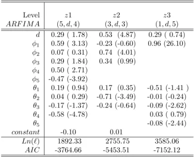
Level z1 z2 z3 ARF IM A (5, d,4) (3, d,3) (1, d,5) d 0.29 ( 1.78) 0.53 (4.87) 0.29 ( 0.74) φ1 0.59 ( 3.13) -0.23 (-0.60) 0.96 (26.10) φ2 0.07 ( 0.31) 0.74 (4.01) φ3 0.29 ( 1.84) 0.34 (0.99) φ4 0.50 ( 2.71) φ5 -0.47 (-3.92) θ1 0.19 ( 0.94) 0.17 (0.35) -0.51 (-1.41 ) θ2 0.04 ( 0.29) -0.71 (-3.49) -0.01 (-0.24) θ3 -0.17 (-1.37) -0.24 (-0.64) -0.09 (-2.62) θ4 -0.58 (-4.78) 0.03 ( 0.79) θ5 -0.08 (-2.44) constant -0.10 0.01 Ln(`) 1892.33 2755.75 3585.06 AIC -3764.66 -5453.51 -7152.12
Table 5: ARFIMA estimation of factor loading series in levels, z1, z2 and
z3 from 04.01.1999 to 25.02.2003. The φ coefficients correspond to the au-toregressive part and the θ coefficients to the moving average part. t-value of the estimated parameters in brackets, Ln(`) is the log-likelihood and (AIC) Akaike Information Criterion.
4.1
Long Memory Models Application
For appropriate representation of the factor loadings series dynamics and the possibility of improved forecasting, we model the long memory in levels and
absolute returns using the ARF IM A, F IGARCH and HY GARCH
mod-els. These models are known to describe volatility reasonably well and pro-vide flexible structure that captures slow decaying autocorrelation functions.
Estimation results with ARF IM A model for series in levels and absolute
returns are reported in Tables 5 and 6 respectively. Estimates ofdare highly
significant across all time series in levels. Thet-statistic are highly significant
to reject the null hypothesis (H0 :d = 0) at 1% significance level. Results for
absolute returns |z2| does confirm earlier tests results in that antipersitence
in |z2|may not be rejected.
Estimation results for the F IGARCH(1, δ,1) and HY GARCH(1, d,1)
models are reported in Tables 7 and 8 respectively. We assume the Student-t
distribution because it can appropriately account for leptokurticity exhibited
by high frequency financial data, Pagan (1996). Under student-t distributed
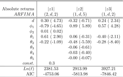
es-Absolute returns |z1| |z2| |z3| ARF IM A (2, d,2) (1, d,5) (1, d,2) d 0.30 ( 4.73) -0.32 (-0.71) 0.24 ( 2.34) φ1 -0.79 (-4.65) 0.89 ( 5.89) 0.57 ( 4.28) φ2 0.01 ( 0.02) θ1 0.61 ( 2.90) 0.06 (-0.31) -0.40 (-2.11) θ2 -0.22 (-1.09) -0.48 (-5.59) -0.28 (-8.40) θ3 -0.06 (-0.61) θ4 -0.03 (-0.40) θ5 -0.00 (-0.07) const. 0.3 Ln(`) 2381.53 2913.99 3927.21 AIC -4753.06 -5813.98 -7846.42
Table 6: ARFIMA estimation of factor loading series in absolute returns,
|z1|, |z2| and |z3| from 04.01.1999 to 25.02.2003. The φ coefficients cor-respond to the autoregressive part and the θ coefficients to the moving av-erage part. t-value of the estimated parameters in brackets, Ln(`) is the log-likelihood and (AIC) Akaike Information Criterion.
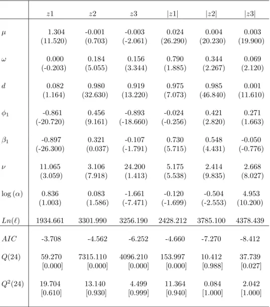
timates indicate long-memory in levels and absolute returns. Besides, the
student-t distribution parameter, ν are significantly different from zero,
in-dicating strong fat tail phenomena. Estimates, δ >0 in F IGARCH models
suggest non-stationary long memory characteristics in levels and absolute re-turns for the first and third factor loadings series, whereas the second series (δ < 0) indicate a stationary long memory behavior. We assess models fit
through the log-likelihood, Ln(`), the Akaike Information Criterion, (AIC)
and the performance of the Box-Pierce (Q2) statistic for testing remaining
se-rial correlation in the squared standardized residuals, McLeod and Li (1983). TheF IGARCH andHY GARCH models perform well in describing the
high persistence existing in the conditional variance. The Q2(24) statistics
suggests that the F IGARCH model can better capture the autocorrelations
in the conditional variance for the series in levels while the HY GARCH is
more appropriate in the case of absolute returns. TheF IGARCH models
re-port higher loglikelihood values for the series in levels while theHY GARCH
values are higher for absolute returns. Moreover, models in absolute returns produce better fit than those in levels, which confirms the findings of Ding et al. (1993), that absolute returns are the most appropriate indicators to represent the long memory volatility processes.
1999 2000 2001 2002 2003 0.6 0.8 1.0 1.2 1.4
ARFIMA(5,0.29,4) fit z1 series PcGive Graphics 17:38:41 25-Jan-2007
1999 2000 2001 2002 2003 -0.025 0.000 0.025 0.050 0.075 0.100 0.125 0.150 0.175
ARFIMA(2,0.3,2) forecasts |z1| series PcGive Graphics 18:51:37 25-Jan-2007
1999 2000 2001 2002 2003 -0.25 -0.20 -0.15 -0.10 -0.05 0.00 0.05
0.10 ARFIMA(3,0.53,3) fit z2 series
PcGive Graphics 14:01:43 31-Jan-2007
1999 2000 2001 2002 2003 0.00 0.05 0.10 0.15 0.20 0.25 0.30
ARFIMA(1,-0.32,5) forecasts |z2| series
PcGive Graphics 19:01:26 25-Jan-2007
1999 2000 2001 2002 2003 -0.100 -0.075 -0.050 -0.025 0.000 0.025 0.050 0.075 0.100 0.125
ARFIMA(1,0.29,5) fit z3 series
PcGive Graphics 14:17:27 31-Jan-2007
1999 2000 2001 2002 2003 0.00 0.01 0.02 0.03 0.04 0.05 0.06 0.07
ARFIMA(1,0.24,2) forecasts |z3| series
PcGive Graphics 19:08:58 25-Jan-2007
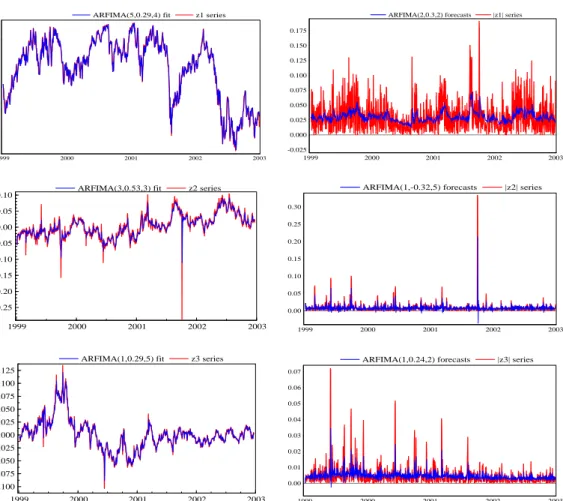
Figure 5: Actual series (red) and in-sample fit (blue) for the estimated
ARF IM A(p, d, q) model in levels and absolute returns. Time interval from
04.01.1999−25.02.2003, with 1039 observations.
We examine the in-sample fit of theARF IM Amodel for the series in
lev-els and absolute returns, Figure 5 as well as the conditional variance forecast
in levels, Figure 6 and absolute returns, Figure 7 for the F IGARCH and
HY GARCH models. Table 9 show in-sample forecast performance evaluated
on the basis of the Root Mean Square Error (RM SE) and the Mean Absolute
Prediction Error (M AP E). The main findings are that theF IGARCH and
HY GARCH models show better forecast performance than the ARF IM A
model and seems to successfully achieve the aim of modeling the long memory behavior of volatility in a parsimonious way.
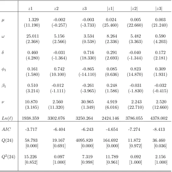
z1 z2 z3 |z1| |z2| |z3| µ 1.329 -0.002 -0.003 0.024 0.005 0.003 (11.190) (-0.257) (-3.733) (25.460) (22.660) (21.240) ω 25.011 5.156 3.534 8.264 5.482 0.590 (2.368) (2.566) (0.538) (2.336) (3.363) (4.203) δ 0.460 -0.031 0.716 0.291 -0.040 0.172 (4.280) (-1.364) (18.330) (2.693) (-1.344) (2.181) φ1 0.161 0.742 -0.865 0.085 0.823 0.309 (1.580) (10.100) (-14.110) (0.636) (14.870) (1.931) β1 0.510 -0.012 -0.261 0.248 -0.031 -0.032 (3.214) (-1.111) (-3.965) (1.586) (-1.830) (-0.415) ν 10.870 2.560 30.965 4.919 2.243 2.520 (3.185) (11.320) (1.349) (6.016) (22.710) (12.660) Ln(`) 1938.359 3302.076 3250.264 2424.146 3786.055 4378.002 AIC -3.717 -6.404 -6.243 -4.654 -7.274 -8.413 Q(24) 58.793 19.167 4095.820 164.692 11.872 36.460 [0.000] [0.691] [0.000] [0.000] [0.972] [0.036] Q2(24) 15.226 0.097 7.319 11.789 0.092 2.156 [0.852] [1.000] [0.998] [0.961] [1.000] [1.000]
Table 7: F IGARCH estimation of the factor loading series in levels and
absolute returns with t statistics in parentheses. Significance is at 5% level. Estimation is with the Student distribution with ν degrees of freedom. Ln(`)
is the value of the maximized likelihood. Q(24)andQ2(24)are the Box-Pierce statistic for remaining serial correlation in the standardized and squared stan-dardized residuals respectively, using 24 lags with p-values in square brackets. The critical value at significant level of 5% is 36.4 .
z1 z2 z3 |z1| |z2| |z3| µ 1.304 -0.001 -0.003 0.024 0.004 0.003 (11.520) (0.703) (-2.061) (26.290) (20.230) (19.900) ω 0.000 0.184 0.156 0.790 0.344 0.069 (-0.203) (5.055) (3.344) (1.885) (2.267) (2.120) d 0.082 0.980 0.919 0.975 0.985 0.001 (1.164) (32.630) (13.220) (7.073) (46.840) (11.610) φ1 -0.861 0.456 -0.893 -0.024 0.421 0.271 (-20.720) (9.161) (-18.660) (-0.256) (2.820) (1.663) β1 -0.897 0.321 -0.107 0.730 0.548 -0.050 (-26.300) (0.037) (-1.791) (5.715) (4.431) (-0.776) ν 11.065 3.106 24.200 5.175 2.414 2.668 (3.059) (7.918) (1.413) (5.538) (9.835) (8.027) log (α) 0.836 0.083 -1.661 -0.120 -0.504 4.953 (1.003) (1.586) (-7.471) (-1.699) (-2.553) (10.200) Ln(`) 1934.661 3301.990 3256.190 2428.212 3785.100 4378.439 AIC -3.708 -4.562 -6.252 -4.660 -7.270 -8.412 Q(24) 59.270 7315.110 4096.210 153.997 10.412 37.739 [0.000] [0.000] [0.000] [0.000] [0.988] [0.027] Q2(24) 19.704 13.140 4.499 11.364 0.084 2.042 [0.610] [0.930] [0.999] [0.940] [1.000] [1.000]
Table 8: HY GARCH estimation of the factor loading series in levels and
ab-solute returns witht statistics in parentheses. Significance is at5% level. Es-timation is with the Student-t distribution with ν degrees of freedom. log (α)
is the log of weight α, to the difference operator(1−L)d. Ln(`) is the value of the maximized likelihood. Q(24) and Q2(24) are the Box-Pierce statistic for remaining serial correlation in the standardized and squared standardized residuals respectively, using 24 lags with p-values in square brackets.
G@RCH Forecasting 01/27/07 17:09:20 Page: 1 of 1 100 200 300 400 500 600 700 800 900 1000 0.0 0.5 1.0 100 200 300 400 500 600 700 800 900 1000 0.0025 0.0050 0.0075
FIGARCH (1,0.46,1) Cond. Var. Forecasts for z1
G@RCH Forecasting 01/31/07 19:32:52 Page: 1 of 1 0 100 200 300 400 500 600 700 800 900 1000 0.0 0.5 1.0 1.5 0 100 200 300 400 500 600 700 800 900 1000 0.0025 0.0050 0.0075
HYGARCH (1,0.89,1) Cond. Var. Forecasts for z1
G@RCH Forecasting 01/31/07 16:59:08 Page: 1 of 1 0 100 200 300 400 500 600 700 800 900 1000 -0.50 -0.25 0.00 0 100 200 300 400 500 600 700 800 900 1000 0.000 0.025 0.050 0.075
FIGARCH (1,-0.03,1) Cond. Var. Forecasts for z2
G@RCH Forecasting 01/31/07 18:07:59 Page: 1 of 1 0 100 200 300 400 500 600 700 800 900 1000 -0.25 0 100 200 300 400 500 600 700 800 900 1000 0.01 0.02 0.03
0.04 HYGARCH (1,0.98,1) Cond. Var. Forecasts for z2
G@RCH Forecasting 01/31/07 18:54:23 0 100 200 300 400 500 600 700 800 900 1000 -0.1 0 100 200 300 400 500 600 700 800 900 1000 0.0005 0.0010 0.0015 0.0020
FIGARCH (1,0.29,1) Cond. Var. Forecasts for z3
G@RCH Forecasting 01/28/07 10:03:25 0 100 200 300 400 500 600 700 800 900 1000 1100 -0.1 0.0 0.1 0.2 0 100 200 300 400 500 600 700 800 900 1000 0.0025 0.0050 0.0075
HYGARCH (1,0.91,1) Cond. Var. Forecasts for z3
Figure 6: Left-Right panels: F IGARCH andHY GARCH conditional
vari-ance forecast of factor loading in levels. Time interval from 04.01.1999−
25.02.2003, with 1039 observations.
G@RCH Forecasting 01/28/07 10:49:27 Page: 1 of 1 0 100 200 300 400 500 600 700 800 900 1000 -0.1 0.0 0 100 200 300 400 500 600 700 800 900 1000 0.002 0.004 0.006
FIGARCH (1,0.29,1) Cond. Var. Forecasts for |z1|
G@RCH Forecasting 01/28/07 10:38:39 Page: 1 of 1 0 100 200 300 400 500 600 700 800 900 1000 -0.1 0.0 0.1 0 100 200 300 400 500 600 700 800 900 1000 0.002 0.004 0.006
HYGARCH (1,0.97,1) Cond. Var. Forecasts for |z1|
G@RCH Forecasting 01/28/07 11:05:59 Page: 1 of 1 0 100 200 300 400 500 600 700 800 900 1000 -0.5 0.0 0 100 200 300 400 500 600 700 800 900 1000 0.000 0.025 0.050 0.075
FIGARCH (1,-0.04,1) Cond. Var. Forecasts for |z2|
G@RCH Forecasting 02/06/07 21:41:23 Page: 1 of 1 0 100 200 300 400 500 600 700 800 900 1000 0.0 0 100 200 300 400 500 600 700 800 900 1000 0.02 0.04
HYGARCH (1,0.98,1) Cond. Var. Forecasts for |z2|
G@RCH Forecasting 02/06/07 21:19:22 Page: 1 of 1 0 100 200 300 400 500 600 700 800 900 1000 -0.1 0.0 0 100 200 300 400 500 600 700 800 900 1000 0.001 0.002 0.003
FIGARCH (1,0.98,1) Cond. Var. Forecasts for |z3|
G@RCH Forecasting 01/28/07 11:42:19 0 100 200 300 400 500 600 700 800 900 1000 0.0 0.1 0 100 200 300 400 500 600 700 800 900 1000 0.0005 0.0010 0.0015
0.0020 HYGARCH (1,0.001,1) Cond. Var. Forecasts for |z3|
Figure 7: Left-Right panels: F IGARCH andHY GARCH conditional
vari-ance forecast of absolute returns. Time interval from04.01.1999−25.02.2003, with 1039 observations.
ARF IM A F IGARCH HY GARCH RM SE z1 0.026 0.171 0.171 z2 0.006 0.001 0.001 z3 0.005 0.001 0.001 |z1| 0.019 0.001 0.001 |z2| 0.007 0.001 0.001 |z3| 0.002 0.001 0.001 M AP E z1 3.180 0.991 0.991 z2 27.600 1.166 0.860 z3 68.720 2.837 9.413 |z1| 52.657 22.910 16.380 |z2| 70.577 1.892 2.409 |z3| 41.706 9.134 10.39
Table 9: In-sample performance of the five-step ahead forecast of the
esti-mated ARF IM A, F IGARCH and HY GARCH models for the factor load-ing series in levels and absolute returns. The measures of forecast accuracy are the Root Mean Square Error (RM SE)and the Mean Absolute Prediction Error (M AP E).
5
Conclusion
We present an empirical investigation of long memory dynamics in the fac-tors of Implied Volatility Strings. The factor loadings series are obtained
by applying a Dynamic Semiparametric Factor Model (DSF M) for implied
volatility strings on the German DAX index market. Long range
depen-dence in the factor loadings series is tested using the rescaled variance V /S
and the semiparametricLobRobtests. We estimated the degree of long
mem-ory based on the log-periodogram GP H regression estimator and the GSP
estimator based on the Whittle approximate maximum likelihood estimate. Results are indicative of long-range dependence in the factor loading series in levels and absolute returns. The factors can be interpreted in terms of a long term, middle long term and short term impact on the dynamics of
IV S. The first factor loading, z1 is highly persistent and influences all
op-tions similarly, irrespective of maturity. The impact of the second factor
loading, z2 gradually diminishes for longer maturities and the third factor
governs large volatility changes in relatively short maturities. Such depen-dence or persistence has importance implications for short-term trading and long range investment strategies. As a consequence, hedging strategies of a long position should take into consideration the long-memory effects in a short position in a call option. This would certainly provide more secure protection against negative effects of long-range persistence in volatility. On the other hand, better results could be obtained for models that price and hedge derivative securities when there is prior information on long-memory volatility in terms of expectation on the potential level of volatility and the rate at which volatility changes.
For an appropriate representation of the series dynamics and the possi-bility of improved forecasting, we model the long memory in volatility via
the class of flexible processes, the ARF IM A,F IGARCH and HY GARCH
models. Our results indicate that these models appear to capture the slow decaying autocorrelation function and therefore are applicable in mimicking the dynamics of the factor loadings. In comparison, models in absolute re-turns have better performance, confirming the findings of Ding et al. (1993), that absolute returns are the most appropriate indicator to represent the long memory volatility processes. It would be interesting to find out if there are persistent time scales that are of local importance or influence the fac-tor loading time series. Therefore, a possible extensions for future research would include studies on spectral analysis or wavelet transform to identify such persistent time scales. In addition, the resulting long range dependence and evidence of fat tail phenomenon also provides a natural extension to
investigate long memory value-at-risk. This would be useful to regulators, derivative market participants and practitioners whose interest is to reason-ably forecast stock market movements.
References
Anderson, T. and Bollerslev, T., (1998): Deutsche Mark-Dollar Volatility: Intraday Activity Patterns, Macroeconomic Announcements, and Long
Run Dependencies. Journal of Finance,53: 219–265.
Baillie, R. T., (1996): Long memory processes and fractional integration in
economics. Journal of Econometrics, 73: 5–59.
Baillie, R. T., Bollerslev, T., Mikkelson, H., (1996): Fractionally
Inte-grated Generalized Autoregressive Conditional Heteroskedasticity.Journal
of Econometrics,14: 3–30.
Beran, J., (1994): Statistics for long memory processes. Chapman & Hall,
New York.
Bhardwaj, G. and Swanson, N.R., (2004): An Empirical Investigation of the Usefulness of ARFIMA Models For Predicting Macroeconomic and
Financial Times series.Working paper, Rutgers University.
Bollerslev, T., (1987): A conditionally heteroskedastic time series model for
speculative prices and rates of returns.Review of Economics and Statistics,
69: 542-547.
Bollerslev, T. and Jubinski, D., (1999): Equity trading volume and volatility:
Latent information arrivals and common long-run dependencies. Journal
of Business and Economic Statistics, 17: 9 - 21.
Bollerslev, T. and Mikkelsen, H., (1996): Modelling and Pricing Long
Mem-ory in Stock Market Volatility. Journal of Econometrics, 73: 151 - 184.
Bollerslev, T., and Wright, J.H., (2000): Semiparametric estimation of
Long-memory volatility dependencies: The role of high-frquency data. Journal
of Econometrics,Vol.98, No.1, pp.81-106.
Borak, S., H¨ardle, W. and Fengler, M., (2005): DSFM fitting of Implied
Volatility Surfaces, Proceedings 5th International Conference on Intelligent System Design and Applications, IEEE Computer Society Number P2286, Library of Congress Number 2005930524.
Borak, S., H¨ardle, W., Mammen, E. and Park, B. U. (2007): Time series
modeling with semiparametric factor dynamics.SFB 649 Discussion Paper
2007-023, Humboldt-Universit¨at zu Berlin.
Brown, R.L., Durbin, J., and Evans, J.M., (1975): Techniques for testing
the constancy of regression relationship over time. Journal of the Royal
Statistical Society B, 37: 149 192.
Cheung, Y. W., and Lai, K. S., (1995): A search for long memory in
interna-tional stock market returns.Journal of International Money and Finance,
14, 597-615.
Chung, C. F., (1999): Estimating the Fractionally Integrated GARCH
Model.working paper, National Ta¨ıwan Univerity.
Davidson, J., (2004): Moments and memory properties of linear conditional
heteroskedasticity models, and a new model.Journal of Business and
Eco-nomic Statistics, 22, 16-29.
Deo, R. S. and Hurvich, C. M., (2001): On the Log Periodogram Regression Estimator of the Memory Parameter in Long Memory Stochastic Volatility
Models.Econometric Theory, 17(686-710).
Diebold, F.X. and Inoue, A., (2001): Long memory and Regime Switching.
Journal of Econometrics, 105, 131–159.
Diebold, F.X. and Rudebusch, G.D., (1991): On the Power of the
Dickey-Fuller Test Against Fractional Alternatives.Economic letters,35, 155–160.
Ding, Z. and Granger, C.W.J., (1996): Modelling Volatility Persistence of
Speculative Returns. A New Approach.Journal of Econometrics,73, 185–
215.
Ding, Z., Granger, C.W.J. and Engle, R.F, (1993): A long memory property
of stock market returns and a new model. Journal of Empirical Finance,
1, 83 - 106.
Doornik, J.A., (2006a): An Introduction to OxMetrics 4. A software System
for Data Analysis and Forecasting. Timberlake Consultant Ltd., first edn.
Doornik, J.A., Ooms, M., (2004): Inference and forecasting for ARFIMA
models with an Application to US and UK inflation. Studies in Nonlinear
Elliott, G., Rothenberg, T. J and Stock, J. H., (1996): Efficient tests for an
autoregressive unit root. Econometrica , 64, 813–836.
Fengler, M., H¨ardle, W. and Mammen, E., (2007): A Semiparametric
Fac-tor Model for Implied Volatility Surface Dynamics. Journal of Financial
Econometrics, Vol.5, No.2,000-000.
Geweke, Porter-Hudak (1983): The Estimation and Application of
Long-Memory Time Series Models.Journal of Time Series Analysis,4, 221-238.
Giacomini, E., Handel, M. and H¨ardle, W., (2006): Time Dependent
Rel-ative Risk Aversion. SFB 649, Discussion paper 2006-020,
Humboldt-Universit¨at zu Berlin.
Giraitis, L., Kokoszka, P. and Leipus, R., (2000): Stationary ARCH models:
Dependence structure and central limit theorem. Econometric Theory 16,
3-22.
Giraitis, L., Kokoszka, P. and Leipus, R., (2001): Testing for long memory in
the presence of a general trend. Journal of Applied Probability, 38, 1033–
1054.
Giraitis, L., Kokoszka, P., Leipus, R. and Teyssi`ere, G., (1999):
Semipara-metric Estimation of the Intensity of Long-Memory in Conditional
Het-eroskedasticity. G.R.E.Q.A.M., 99a24, Universite Aix-Marseille III.
Ghysels, E., Santa-Clara, P. and Valkanov (2004): Predicting Volatility:
Get-ting the Most out of Return Data Sampled at Different Frequencies.
Sci-entific Series, 2004s–19.
Granger, C.W.J., (1980): Long memory relationships and the aggregation of
dynamic models. Journal of Econometrics, 14: 261–279.
Granger, C.W.J. and Ding, Z., (1995): Some properties of absolute returns:
An alternative measure of risk.Annales d’E´conomie et de Statistique,40,
67 - 91.
Granger, C.W.J. and Ding, Z., (1996): Varieties of Long-Memory Models.
Journal of Econometrics, 73, 61–77.
Granger, C. W. J. and Joyeux, R., (1995): An introduction to long memory
times series models and fractional differencing. Journal of Time Series
Hall, P., H¨ardle, W., Kleinow, T. and Schmidt, P., (2000): Semiparametric Bootstrap Approach to Hypothesis Tests and Confidence Intervals for the
Hurst Coefficient.Statistical Inference for Stochastic Processes,3, 263-276.
Herzberg, M., Sibbertsen, P., (2004): Pricing of options under different
volatility models. Technical Report/ Universit¨at Dortmund, SFB 475,
Komplexit¨atsreduktion in Multivariaten Datenstrukturen, 2004,62.
Hillebrand, E., (2005): Neglecting parameter changes in GARCH models.
forthcoming. Journal of Econometrics, 129.
Hosking, J.R.M., (1981): Fractional Differencing. Biometrika, 68(1),
165-176.
Hurvich, C., Doe, R. and Brodsky, J., (1998): The Mean Square Error of Geweke and Porter-Hudak’s estimator of the Memory Parameter of a
Long-Memory time series. Journal of Time Series Analysis, 19, 19-46.
Laurent, S. and Peters, J. P., (2002): Garch 2.2: An Ox Package for
estimat-ing and forecastestimat-ing Various ARCH Models.Journal of Economic Surveys,
16(3), 447–485.
Lobato, I. and P.M. Robinson (1998): A Nonparametric Test for I(0).Review
of Economic Studies, 65(3), 475495.
Lobato, I. and N.E. Savin (1998): Real and Spurious Long-Memory
Proper-ties of Stock Market Data. Journal of Business and Economic Statistics,
16, 261-283.
MacKinnon, J. G., (1991): Critical values for cointegration tests.in C. W. J.
Granger R. F. Engle (eds),Long-Run Economic Relationships, Oxford
Uni-versity Press, Oxford.
McLeod, A. I. and Li, W. K., (1983): Diagnostic checking ARMA time series
models using squared residual autocorrelations. Journal of Time Series
Analysis, 4, 269-273.
Mandelbrot, B. B., (1971): When a price be arbitraged efficiently? a limit
to the validity of the random walk and Martingale models.Review of
Eco-nomics and Statistics,53, 225-236.
Mikosch, T., Starica, C., (2004): Nonstationarities in financial time series,
the long range dependence and the IGARCH effects. Review of Economics
Newey, W.K. and West, K.D., (1994): A Simple Positive Definite,
Het-eroskedasticity and Autocorelation Consistent Covariance Matrix.
Econo-metrica, 55, 703–705.
Newey, W.K. and West, K.D., (1994): Automatic lag selection in covariance
matrix estimation. Review of Economic Studies, 61, 631–653.
Pagan, A., (1996): The econometrics of financial markets.Journal of
Empir-ical Finance, 3, 15–102.
Phillips, P.C.B and Shimotsu, K., (2004): Local Whittle estimation in
non-stationary and unit root cases. Annals of Statistics, 32, 656–692.
Robinson, P.M., (1995a): Gaussian Semiparametric Estimation of
Long-Range Dependence.Annals of Statistics, 23, 1630-1661.
Robinson, P.M., (1995b): Log-Periodogram regression of time Series with
Long Range Dependence. Annals of Statistics, 23(3), 1048-1072.
Robinson, P.M., (2003): Long memory time series. In Robinson, P.M. (Ed.),
Times series with Long Memory.Oxford University Press, Oxford.
Robinson, P.M., Henry, M., (1999): Long and Short Memory Conditional
Heteroskedasticity in Estimating the Memory Parameter in Levels.
Eco-nomic Theory, 15, 299-336.
Ryd´en, T., Ter¨asvirta, T. and ˙Asbrink, S (1998): Stylized facts of daily
return series and hidden Markov model.Journal of Applied Econometrics,
13: 217-244.
Sibbertsen, P., (2004): Long-Memory in Volatilities of German Stock
Re-turns. Empirical Economics , 29, 477 - 488.
Tiao, G. C. (2001): Univariate Autoregressive Moving-Average Models. In Pena, D., Tiao, G.C. and Tsay, R.S. (eds.), A Course in Time Series Analy-sis.ew York (Wiley), Chapter 3.
Velasco, C., (1999): Gaussian Semiparametric Estimation of Non-Stationary
Time Series.Journal of Time Series Analysis,20: 87 127(41).
Velasco, C., (1999): Non-Stationary Log-periodogram Regresssion. Journal
of Econometrics,91: 325 - 371.
Wilson, P. J., and Okunev, J., (1999): Long-Term Dependencies and Long
Run Non-Periodic co-Cycles: Real Estate and Stock Markets. Journal of
SFB 649 Discussion Paper Series 2007
For a complete list of Discussion Papers published by the SFB 649, please visit http://sfb649.wiwi.hu-berlin.de.
001 "Trade Liberalisation, Process and Product Innovation, and Relative Skill Demand" by Sebastian Braun, January 2007.
002 "Robust Risk Management. Accounting for Nonstationarity and Heavy Tails" by Ying Chen and Vladimir Spokoiny, January 2007.
003 "Explaining Asset Prices with External Habits and Wage Rigidities in a DSGE Model." by Harald Uhlig, January 2007.
004 "Volatility and Causality in Asia Pacific Financial Markets" by Enzo Weber,
January 2007.
005 "Quantile Sieve Estimates For Time Series" by Jürgen Franke, Jean-Pierre Stockis and Joseph Tadjuidje, February 2007.
006 "Real Origins of the Great Depression: Monopolistic Competition, Union Power, and the American Business Cycle in the 1920s" by Monique Ebell and Albrecht Ritschl, February 2007.
007 "Rules, Discretion or Reputation? Monetary Policies and the Efficiency of Financial Markets in Germany, 14th to 16th Centuries" by Oliver Volckart, February 2007.
008 "Sectoral Transformation, Turbulence, and Labour Market Dynamics in Germany" by Ronald Bachmann and Michael C. Burda, February 2007. 009 "Union Wage Compression in a Right-to-Manage Model" by Thorsten
Vogel, February 2007.
010 "On σ−additive robust representation of convex risk measures for
unbounded financial positions in the presence of uncertainty about the market model" by Volker Krätschmer, March 2007.
011 "Media Coverage and Macroeconomic Information Processing" by Alexandra Niessen, March 2007.
012 "Are Correlations Constant Over Time? Application of the CC-TRIGt-test
to Return Series from Different Asset Classes." by Matthias Fischer, March 2007.
013 "Uncertain Paternity, Mating Market Failure, and the Institution of Marriage" by Dirk Bethmann and Michael Kvasnicka, March 2007.
014 "What Happened to the Transatlantic Capital Market Relations?" by Enzo Weber, March 2007.
015 "Who Leads Financial Markets?" by Enzo Weber, April 2007. 016 "Fiscal Policy Rules in Practice" by Andreas Thams, April 2007.
017 "Empirical Pricing Kernels and Investor Preferences" by Kai Detlefsen, Wolfgang Härdle and Rouslan Moro, April 2007.
018 "Simultaneous Causality in International Trade" by Enzo Weber, April 2007.
019 "Regional and Outward Economic Integration in South-East Asia" by Enzo Weber, April 2007.
020 "Computational Statistics and Data Visualization" by Antony Unwin, Chun-houh Chen and Wolfgang Härdle, April 2007.
021 "Ideology Without Ideologists" by Lydia Mechtenberg, April 2007.
022 "A Generalized ARFIMA Process with Markov-Switching Fractional Differencing Parameter" by Wen-Jen Tsay and Wolfgang Härdle, April 2007.
SFB 649, Spandauer Straße 1, D-10178 Berlin http://sfb649.wiwi.hu-berlin.de
SFB 649, Spandauer Straße 1, D-10178 Berlin http://sfb649.wiwi.hu-berlin.de
This research was supported by the Deutsche
023 "Time Series Modelling with Semiparametric Factor Dynamics" by Szymon Borak, Wolfgang Härdle, Enno Mammen and Byeong U. Park,
April 2007.
024 "From Animal Baits to Investors’ Preference: Estimating and Demixing of the Weight Function in Semiparametric Models for Biased Samples" by Ya’acov Ritov and Wolfgang Härdle, May 2007.
025 "Statistics of Risk Aversion" by Enzo Giacomini and Wolfgang Härdle,
May 2007.
026 "Robust Optimal Control for a Consumption-Investment Problem" by Alexander Schied, May 2007.
027 "Long Memory Persistence in the Factor of Implied Volatility Dynamics" by Wolfgang Härdle and Julius Mungo, May 2007.