This is an author-deposited version published in: http://oatao.univ-toulouse.fr/ Eprints ID: 8328
To link to this article: DOI: 10.1214/10-EJS576 URL: http://dx.doi.org/10.1214/10-EJS576
To cite this version:
Bigot, Jérémie and Gadat, Sébastien and Marteau,
Clément
Sharp template estimation in a shifted curves model. (2010)
Electronic Journal of Statistics, vol. 4. pp. 994-1021. ISSN 1935-7524
O
pen
A
rchive
T
oulouse
A
rchive
O
uverte (
OATAO
)
OATAO is an open access repository that collects the work of Toulouse researchers and makes it freely available over the web where possible.
Any correspondence concerning this service should be sent to the repository administrator: [email protected]
Sharp template estimation in a shifted curves model
Jérémie Bigot, Sébastien Gadat & Clément Marteau Institut de Mathématiques de Toulouse Université de Toulouse et CNRS (UMR 5219)
31062 Toulouse, Cedex 9, France
{Jeremie.Bigot,Sebastien.Gadat,Clement.Marteau}@math.univ-toulouse.fr, August 3, 2010
Abstract
This paper considers the problem of adaptive estimation of a template in a randomly shifted curve model. Using the Fourier transform of the data, we show that this problem can be transformed into a linear inverse problem with a random operator. Our aim is to approach the estimator that has the smallest risk on the true template over a finite set of linear estimators defined in the Fourier domain. Based on the principle of unbiased empirical risk minimization, we derive a nonasymptotic oracle inequality in the case where the law of the random shifts is known. This inequality can then be used to obtain adaptive results on Sobolev spaces as the number of observed curves tend to infinity. Some numerical experiments are given to illustrate the performances of our approach.
Keywords: Template estimation, Curve alignment, Inverse problem, Random operator, Oracle inequality, Adaptive estimation.
1
Introduction
1.1 Model and objectives
The goal of this paper is to study a special class of linear inverse problems with a random operator. We consider the problem of estimating a curve f, called template or shape function, from the observations ofnnoisy and randomly shifted curvesY1, . . . Yncoming from the following
Gaussian white noise model:
dYj(x) =f(x−τj)dx+ǫdWj(x), x∈[0,1], j= 1, . . . , n (1.1)
where Wj are independent standard Brownian motions on [0,1], ǫ represents a level of noise
common to all curves, the τj’s are unknown random shifts independent of the Wj’s, f is the
unknown template to recover, and nis the number of observed curves that may be let going to infinity to study asymptotic properties. This model is realistic in many situations where it is reasonable to assume that the observed curves represent replications of almost the same process and when a large source of variation in the experiments is due to transformations of the time axis. Such a model is commonly used in many applied areas dealing with functional data such as neuroscience (see e.g. Isserles, Ritov and Trigano (2008)) or biology (see e.g. Ronn (1998)). A well known problem in functional data analysis is the alignment of similar curves that differ by a time transformation to extract their common features, and (1.1) is a simple model where
f represents such common features (see Ramsay and Silverman (2002), Ramsay and Silverman (2005) for a detailed introduction to curve alignment problems in statistics).
The function f :R→Ris assumed to be of period1 so that the model (1.1) is well defined, and the shifts τj are supposed to be independent and identically distributed (i.i.d.) random
the paper, it is supposed that the density g is known. Estimating f can be seen as an inverse problem with a random operator. Indeed, the template f is not observed directly, but through
nindependent realizations of the random operator Aτ :L2per([0,1])→L2per([0,1]) defined by
Aτ(f)(x) =f(x−τ), x∈[0,1],
whereL2
per([0,1])denotes the space of squared integrable functions on[0,1]with period 1, andτ
is random variable with densityg. The additive Gaussian noise makes this problem ill-posed, and Bigot and Gadat (2010) have shown that estimating f in such models is in fact a deconvolution problem where the densityg of the random shifts plays the role of the convolution operator. For theL2 risk on [0,1], Bigot and Gadat (2010) have derived the minimax rate of convergence for the estimation of f over Besov balls as n tends to infinity. This minimax rate depends both on the smoothness of the template and on the decay of the Fourier coefficients of the densityg. This is a well known fact for standard deconvolution problem in statistics, see e.g. Fan (1991), Donoho (1995), but the results in Bigot and Gadat (2010) represent a novel contribution and a new point of view on template estimation in inverse problems with a random operator such as (1.1). This appears also to be a new setting in the field of inverse problem with partially known operators as considered in Cavalier and Hengartner (2005), Efromovich and Koltchinskii (2001), Hoffmann and Reiß (2008), Marteau (2006) and Cavalier and Raimondo (2007).
However, the approach followed in Bigot and Gadat (2010) is only asymptotic, and the main goal of this paper is to derive non-asymptotic results to study the estimation of f by keeping fixed the number nof observed curves.
1.2 Fourier Analysis and an inverse problem formulation
Supposing that f ∈L2per([0,1]), we denote byθk its kth Fourier coefficient, namely:
θk=
Z 1 0
e−2ikπxf(x)dx.
In the Fourier domain, the model (1.1) can be rewritten as
cj,k :=
Z 1 0
e−2ikπxdYj(x) =θke−i2πkτj+ǫzk,j (1.2)
where zk,j are i.i.d. NC(0,1) variables, i.e. complex Gaussian variables with zero mean and
such that E|zk,j|2 = 1. This means that the real and imaginary parts of the zk,j ’s are Gaussian variables with zero mean and variance 1/2. Thus, we can compute the sample mean of the kth
Fourier coefficient over thencurves as ˜ ck := 1 n n X j=1 ck,j =θkγ˜k+ ǫ √ nξk, (1.3) where ˜ γk:= 1 n n X j=1 e−i2πkτj, (1.4) and the ξk’s are i.i.d. complex Gaussian variables with zero mean and variance 1. The Fourier
coefficients ˜ck in equation (1.3) can be viewed as observations coming from a statistical inverse
problem. Indeed, the standard sequence space model of an ill-posed statistical inverse problem is (see Cavalier, Golubev, Picard and Tsybakov (2002) and the references therein)
ck =θkγk+σzk, (1.5)
where theγk’s are eigenvalues of a known linear operator,zkare random noise variables and σis
is to recover the coefficients θk from the observations ck under various conditions on the decay
to zero of theγk’s as|k| →+∞. A large class of estimators for the problem (1.5) can be written
as ˆ θk=λk ck γk ,
where λ= (λk)k∈Z is a sequence of reals called filter. Various estimators of this form have been
studied in a number of papers, and we refer to Cavalier et al. (2002) for more details. In a sense, we can view equation (1.3) as a linear inverse problem (with σ = √ǫ
n) with a
stochastic operator whose eigenvalues ˜γk = n1Pjn=1e−i2πkτj are random variables that are not observed. Nevertheless, it is supposed that the density g of the shifts is known. Therefore, one can compute the expectation γk of the random eigenvaluesγ˜k given by
γk:=Eγ˜k=E e−i2πkτ= Z +∞ −∞ e−i2πkxg(x)dx.
Hence, if we assume that the density gof the random shifts is known, estimation of the Fourier coefficients of f can be obtained by a deconvolution step of the form
ˆ θk=λk ˜ ck γk , (1.6)
where ˜ck is defined in (1.3) and λ= (λk)k∈Z is a filter whose choice will be discussed later on.
Theoretical properties and optimal choices for the filter λ are presented in the case where the coefficientsγk are known. Such a framework is commonly used in inverse problems such as (1.5)
to obtain consistency results and to study asymptotic rates of convergence, where it is generally supposed that the law of the additive error is Gaussian with zero mean and knownvariance σ2, see e.g Cavalier et al. (2002). In model (1.1), the random shifts may be viewed as a second source of noise and for the theoretical analysis of this problem the law of this other random noise is also supposed to be known.
Recently, some papers have addressed the problem of regularization with partially known operator. For instance, Cavalier and Hengartner (2005) consider the case where the eigenvalues are unknown but independently observed. They deal with the model:
ck=γkθk+ǫξk, ˜γk=γk+σηk, ∀k∈N, (1.7)
where (ξk)k∈Nand(ηk)k∈N denote i.i.d standard gaussian variables. In this case, each coefficient θk can be estimated by γ˜−k1ck. Similar models have been considered in Cavalier and Raimondo
(2007), Marteau (2006) or Marteau (2009). In a more general setting, we may refer to Efromovich and Koltchinskii (2001) and Hoffmann and Reiß (2008).
In this paper, our framework is slightly different in the sense that the operator is stochastic, but the regularization is operated using deterministic eigenvalues. Hence the approach followed in the previous papers is no directly applicable to model (1.1). We believe that estimatingf and deriving convergence rates in model (1.1) without the knowledge of g remains a difficult task, and this paper is a first step to address this issue.
1.3 Previous work in template estimation and shift recovery
The problem of estimating the common shape of a set of curves that differ by a time trans-formation is usually referred to as the curve registration problem, and it has received a lot of attention in the literature over the last two decades. Among the various methods that have been proposed, one can distinguish between landmark-based approaches which aim at aligning common structural points of the curves (typically locations of extrema) see e.g Gasser and Kneip (1992), Gasser and Kneip (1995), Bigot (2006), and nonparametric modeling of the warping functions to align a set of curves see e.g Ramsay and Li (2001), Wang and Gasser (1997), Liu
and Müller (2004). However, in these papers, studying consistent estimates of the common shape
f as the number of curves ntends to infinity is generally not considered.
In the simplest case of shifted curves, various approaches have been developed. Self-modelling regression methods proposed by Kneip and Gasser (1988) are semiparametric models where each observed curve is a parametric transformation of a common regression function. Such models are usually referred to as shape invariant models and estimation in this setting is usually done by iterating the following two steps: estimation of the parameters of the transformations (here the shifts) given a reference curve, and nonparametric estimation of a template by aligning the observed curves given a set of known transformation parameters. Kneip and Gasser (1988) studied the consistency of such a two steps procedure in an asymptotic framework where both the number of functionsn and the number of observed points per curves grows to infinity. Due to the asymptotic equivalence between the white noise model and nonparametric regression with an equi-spaced design (see Brown and Low (1996)), such an asymptotic framework in our setting would correspond to the case where both n tends to infinity and ǫ is let going to zero. In this paper we prefer to focus only on the case wherenmay be let going to infinity, and to leave fixed the level of additive noise in each observed curve.
Based on a model with curves observed at discrete time points, semiparametric estimation of the shifts and the shape function is proposed in Gamboa, Loubes and Maza (2007) and Vimond (2010) as the number of observations per curve grows, but with a fixed number n of curves. A generalization of this approach for the estimation of scaling, rotation and translation parameters for two-dimensional images is also proposed in Bigot, Gamboa and Vimond (2009), but also with a fixed number of observed images. Semiparametric and adaptive estimation of a shift parameter in the case of a single observed curve in a white noise model is also considered by Dalalyan, Golubev and Tsybakov (2006) and Dalalyan (2007). Estimation of a common shape for randomly shifted curves and asymptotic innis considered in Ronn (1998) from the point of view of semiparametric estimation when the parameter of interest is infinite dimensional.
However, in all the above cited papers rates of convergence or oracle inequalities for the estimation of the template are generally not studied. Moreover, our procedure differs from the approaches classically used in curve registration as our estimator is obtained in only one very simple step, and it is not based on an alternative scheme between estimation of the shifts and averaging of back-transformed curves given estimated values of the shifts parameters.
Finally, note that Castillo and Loubes (2009) and Isserles et al. (2008) consider a model similar to (1.1), but they rather focus on the the estimation of the density g of the shifts as n
tends to infinity. Using such an approach could be a good start for studying the estimation of the templatef without the knowledge ofg. However, we believe that this is far beyond the scope of this paper, and we prefer to leave this problem open for future work.
1.4 Organization of the paper
In Section 2, we consider an estimator of the shape function f using monotone filters when the eigenvalues γk are known. Based on the principle of unbiased risk minimization developed
by Cavalier et al. (2002), we propose a data-based choice for the filter λ in (1.6). Then, we derive an oracle inequality showing that the resulting estimator has a risk close to an ideal one when choosing λ over a class of monotone filters. In Section 3, as an example, we study the case of projection filters. This gives an estimator based on the Fourier transform of the curves with a data-based choice of the frequency cut-off. We study its asymptotic properties in terms of minimax rates of converge over Sobolev balls. Finally in Section 4, a detailed simulation study is proposed to illustrate the numerical properties of such estimators. All proofs are deferred to a technical section at the end of the paper.
2
Estimation of the common shape
In the following, we assume that the Fourier coefficients γk are known. In this situation it is
possible to choose a data-dependent filter λ⋆ that mimics the performances of an optimal filter
λ0 called oracle that would be obtained if we knew the true template f. The performances of this filter are related to the performances of the filterλ0 via an oracle inequality. In this section, most of our results are non-asymptotic and are thus related to the approach proposed in Cavalier et al. (2002) to study standard statistical inverse problems via oracle inequalities.
2.1 Smoothness assumptions for the density g
In a deconvolution problem, it is well known that the difficulty of estimating f is quantified by the decay to zero of theγk’s as|k| →+∞. Depending how fast these Fourier coefficients tend
to zero as |k| →+∞, the reconstruction of f will be more or less accurate. This phenomenon was systematically studied by Fan (1991) in the context of density deconvolution. In this paper, the following type of assumption on gis considered:
Assumption 2.1 The Fourier coefficients ofghave a polynomial decay i.e. for some realβ ≥0, there exists two constants Cmax ≥Cmin>0 such that for all k∈Z
Cmin|k|−β ≤ |γk| ≤Cmax|k|−β. (2.1)
2.2 Risk decomposition
Recall that an estimator of the θk’s is given by θˆk = λkγ−k1˜ck, k ∈ Z, see equation (1.6),
where λ = (λk)k∈Z is a real sequence. Examples of commonly used filters include projection
weights λk = 11|k|≤j for some integer j, and the Tikhonov weights λk = 1/(1 + (|k|/ν2)ν1) for some parameters ν1 >0 and ν2 >0. Based on the θˆk’s, one can estimate the signal f using the
Fourier reconstruction formula
ˆ fλ(x) = X k∈Z ˆ θke−2ikπx.
The problem is then to choose the sequence (λk)k∈Z in an optimal way with respect to an
appropriate risk. For a given filter λ we use the classical ℓ2-norm to define the risk of the estimatorθˆ(λ) = (ˆθk)k∈Z R(θ, λ) =Eθkθˆ(λ)−θk2 2 =Eθ X k∈Z |θˆk−θk|2 (2.2)
Note that analyzing the above risk (2.2) is equivalent to analyze the mean integrated square risk R( ˆfλ, f) = Ekfˆλ−fk2 = ER01( ˆfλ(x)−f(x))2dx
. The following lemma gives the bias-variance decomposition ofR(λ, θ). A detailed proof can be found in Bigot and Gadat (2010).
Lemma 2.1 For any given nonrandom filter λ, the risk of the estimator θˆ(λ)can be decomposed as R(θ, λ) =X k∈Z (λk−1)2|θk|2 | {z } Bias + 1 n X k∈Z λ2k ǫ 2 |γk|2 | {z } V1 +1 n X k∈Z λ2k|θk|2 1 |γk|2 − 1 | {z } V2 (2.3)
For a fixed number of curvesnand a given shape functionf, the problem of choosing an optimal filter in a set of possible candidates is to find the best trade-off between low bias and low variance in the above expression. However, this decomposition does not correspond exactly to the classical bias-variance decomposition for linear inverse problems. Indeed, the variance term in (2.3) is the sum of two terms and differs from the classical expression of the variance for linear estimator in
statistical inverse problems. Using our notations, the classical variance term isV1 = ǫ 2 n X k∈Z λ2k |γk|2
and appears in most of linear inverse problems. However, contrary to standard inverse problems, the variance term of the risk also depends on the Fourier coefficientsθkof the unknown function
f to recover. Indeed, our dataγk−1˜ck are noisy observations of θk:
γk−1˜ck=θk+ ˜ γk γk − 1 θk+ ǫ √ nγ −1 k ξk. (2.4)
Hence, using the sequence (γk)k∈N instead of (˜γk)k∈N introduces an additional error. This
ex-plains the presence of the second termV2.
A similar phenomenon occurs with the model (1.7), although it is more difficult to quantify it. Indeed, in this setting:
˜ γk−1ck=θk+ γk ˜ γk − 1 θk+ǫ˜γk−1ξk, ∀k∈N. (2.5)
Hence, we also observe an additional term depending onθ. This term is controlled using a Taylor expansion but the quadratic risk cannot be expressed in a simple form. Let us stress that the difficulty of studying problem (2.5), when compared to our estimator (2.4), comes from the fact that in (2.5) there is a random term in the denominator. We refer to Marteau (2009) for a discussion with some numerical simulation and to Cavalier and Hengartner (2005), Efromovich and Koltchinskii (2001), Hoffmann and Reiß (2008), Marteau (2006) and Cavalier and Raimondo (2007).
2.3 An oracle estimator and unbiased estimation of the risk (URE)
Suppose that one is given a set Λ of cardinalityN ≥1 of possible candidate filters, that is Λ = (λj)
j∈{1,...,N}, with λj = (λjk)k∈Z, j = 1, . . . , N which satisfy some general conditions to
be discussed later on. In the case of projection filters, Λ can be for example the set of filters
λjk =11|k|≤j, k∈Zfor j= 1, . . . , N.
Given a set of filters Λ, the best estimator is defined as the filterλ0 (called oracle) which has the smallest riskR(θ, λ) overΛ, that is
λ0 := arg min
λ∈ΛR(θ, λ). (2.6) This filter is an ideal one because it cannot be computed in practice as the sequence of coefficients
θ is unknown. However, the oracle λ0 can be used as a benchmark to evaluate the quality of a data-dependent filter λ⋆ chosen in the set Λ. This is the main interpretation of the oracle inequality that we will develop in the next section.
2.4 Oracle inequalities for monotone filters
2.4.1 Definitions
First, let us introduce the following class of monotone filters: Λmon := ( λ= (λk)k∈Z:λk=λ−k, X k∈Z λ2k <+∞, 1≥λ0 ≥λ1≥. . .≥λm ≥. . .≥0 ) ,
In practice, the filters λin the set Λ are such that λk = 0 (or vanishingly small) for all k large
enough. Hence, for such choices of filters, numerical minimization of criterions such as (2.6) is feasible, since it only involves the computation of finite sums. Let us thus define the following threshold m0 beyond which all values of the filters λinΛ vanish
m0 = inf k:|γk|2 ≤ log2n n −1. (2.7)
Then,Λis supposed to be a finite set of cardinalityN of monotone filtersλwhich satisfiesλk= 0
as soon as|k| ≥m0, that is
Assumption 2.2 For N ≥ 1, Λ = (λj)j∈{1,...,N} ⊂ ΛNmon with λjk = 0 for |k| ≥ m0 and j= 1, . . . , N.
The choice of the filter λ⋆ will be obtained by minimization of a data-based criterion whose derivation is guided by the unbiased risk estimate (URE) minimization principle developed by Cavalier et al. (2002). Typically, one cannot minimize such a criterion over filters (λk)k∈Z of
infinite length. Indeed, each coefficient θk is estimated by γk−1˜ck where γk = Eγ˜k. Hence, the
ratio γk−1γ˜k should be as close as possible to 1. Since γk→0ask→+∞and the variance ofγ˜k
is equal to n1 + (1−n1)|γk|2, it is clear that large values of kshould be discarded. Bounds similar
to (2.7) on the maximum number of non-vanishing values for the filters are used in papers related to partially known operator, see for instance Cavalier and Hengartner (2005) or Efromovich and Koltchinskii (2001). This bounds have to be carefully chosen but are not of first importance. In general, estimating the operator is easier than estimating the function f.
In this paper, we have chosen to present an adaptive estimator based on the URE principle. Given the finite familyΛ, our aim is to select the best possible filter among this family. We are aware that different adaptive schemes are available in the literature. For instance, the penalized blockwise Stein’s rule (see Marteau (2006) and references therein) provides a filter for the model (1.5) leading to an oracle inequality among all monotone filters. In some sense, the generalization of such kind of result to our model would be more powerful. Nevertheless, we think that our approach is also interesting in this setting since it does not impose a particular regularization scheme. Moreover, the differences between model (1.5) and model (1.3) are easier to underline with our method.
2.4.2 Adaptive regularization scheme
Let us now explain how to compute an estimator U(Y, λ) of the risk R(θ, λ). First, recall that Lemma 2.1 yields the following expression of the quadratic riskR(θ, λ)
R(θ, λ) = X k∈Z (1−λk)2|θk|2 | {z } :=Bias +ǫ 2 n X k∈Z λ2k|γk|−2 | {z } :=V1 +1 n X k∈Z λ2k|θk|2 1 |γk|2 − 1 | {z } :=V2 ,
and suppose that it is possible to construct an estimator Θˆ2k of |θk|2 from the observations of
the shifted curves Y = (Yi)i=1...n. For any non-random filter λ satisfying Assumption 2.2, by
replacing |θk|2 in (2.3) by Θˆ2k, the above decomposition of the risk R(θ, λ) suggests to compute
a data-based criterion U(Y, λ) (depending only on (Y, λ)) of the form
U(Y, λ) := X |k|≤m0 (λ2k−2λk) ˆΘ2k+ ǫ2 n X |k|≤m0 λ2k|γk|−2+ 1 n X |k|≤m0 λ2k|γk|−2Θˆ2k. (2.8)
The criterion U(Y, λ) is thus an approximation of R(θ, λ)− kθk2
2. Then, for choosing a data-dependent filter λ⋆, the principle of URE, see Cavalier et al. (2002) for further details, simply suggests to minimize the criterion U(Y, λ) over λ∈Λ. Following the principle of URE, a data-dependent choice of λwould thus be given by
λ⋆:= arg min
λ∈ΛU(Y, λ). (2.9) In the following, we useΘˆ2
k=γk−2 h |˜ck|2−ǫ 2 n i
as an estimator of|θk|2. Remark thatEθΘˆ2k6=|θk|2.
rather use the principle of minimization of a risk estimate. Nevertheless, we will prove that this bias can be controlled, and that it is in some sense negligible compared toR(θ, λ).
Note that in for the computation ofU(Y, λ), we have taken into account all the terms (Bias,V1 andV2) in the decomposition of the riskR(θ, λ). Unfortunately, when usingΘˆ2k =γk−2
h
|c˜k|2−ǫ
2
n
i
as an estimator of |θk|2, minimization of such a criterion does not lead to satisfactory results.
This is due the term n1Pk∈Zλ2k|γk|−4|
n
|c˜k|2− ǫ
2
n
o
in (2.8) which is an estimation of the variance term V2 in the decomposition (2.3) of the risk R(θ, λ). The main issue is that the study of this term requires a control of |γk|−4, and not only |γk|−2 as for the study of the classical variance
term V1 = ǫ
2
n
P
k∈Zλ2k|γk|−2 in standard inverse problem. Nevertheless, by definition (2.7), one
has that logn2(n)γk−2 ≤ 1 for all |k| ≤ m0. Therefore, this suggests to rather consider filters minimizing a criterion of the form
U1(Y, λ) := X |k|≤m0 (λ2k−2λk)|γk|−2 |c˜k|2− ǫ2 n +ǫ 2 n X |k|≤m0 λ2k|γk|−2 +log 2(n) n X |k|≤m0 λ2k|γk|−4 |˜ck|2− ǫ2 n . (2.10)
Alternatively, following Cavalier and Hengartner (2005), it is sometimes possible to neglect the error generated by the use of an approximation of the unknown random eigenvalues ˜γk by
γk which yet corresponds to the termV2. Indeed, remark that one may findρ >0such that V2≤ 1 n X k∈Z λ2k|θk|2 |γk|2 ≤ 1 nkθk 2sup k∈Z λ2k|γk|−2≤ρkθk2 1 n X k∈Z λ2k|γk|−2=ρkθk2 V1 ǫ2.
Hence, depending on the values of ρ, ǫ2 and kθk2, the variance term V2 may be negligible compared to V1. In this case, one could rather consider the following criterion U0(Y, λ) derived from the decomposition on the classic quadratic risk (i.e. Bias +V1), and defined as
U0(Y, λ) := X |k|≤m0 (λ2k−2λk)|γk|−2 |˜ck|2− ǫ2 n +ǫ 2 n X |k|≤m0 λ2k|γk|−2. (2.11)
In the sequel, we summarize these two approaches by considering the more general criterion
Uα(Y, λ)given by Uα(Y, λ) := X k∈Z (λ2k−2λk)|γk|−2 |˜ck|2− ǫ2 n +ǫ 2 n X k∈Z λ2k|γk|−2+α log2n n X k∈Z λ2k|γk|−4 |˜ck|2− ǫ2 n . (2.12) where 0 ≤ α ≤ 1 is a parameter to be discussed. All the following results of the paper are given for any value of the parameter α in[0,1]. Following the URE principle, we will study the theoretical properties of the filters λ⋆
α ∈Λ defined as
λ⋆α = arg min
λ∈ΛUα(Y, λ). (2.13) for 0 ≤ α ≤ 1. Note that Uα(Y, λ) can be written as a penalized version of the empirical risk
U(Y, λ) defined in (2.8). Choosing the regularization parameter α is a data-driven way is a delicate problem in nonparametric statistics. Nevertheless, the following heuristic arguments can be given for a suitable choice of α. The presence of the additional penalized term V2 is due to the variability along the time axis (random translation) of the template f. When ǫis small compared to kθk2, the white noise deconvolution may be considered as negligible comparing to the alignment issue of the observed curves. the mean error will be larger when the signal to reconstruct possesses a large number of modes. Thus, in a framework with a smallǫand a large
kθk2, it may be reasonable to chooseα 6= 0. To the contrary, if the level of noiseǫis large, the model (1.1) can certainly be considered as being close to the standard white noise deconvolution problem. In this setting, setting α = 0 may be recommended. Moreover, an optimal choice of
α is certainly related to the number of observed curves n. The problem of choosing α is thus discussed in detail in Section 4 on numerical experiments.
2.4.3 Sharp estimator of the oracle risk
We are now able to propose an adaptive estimator of θ. In the following, α will belong to [0,1]and we denote by θα⋆ the estimator related to the filters λ⋆α defined in (2.13) that is
θ⋆k,α= ˜ck
γk
λ⋆k,α for θ⋆α= (θk⋆)k∈Z and λ⋆α = (λ⋆k,α)k∈Z. (2.14)
To simplify the notations, we omit the dependency of θ⋆α and λ⋆α on α, and write θ⋆ =θα⋆ and
λ⋆ =λ⋆α. Through a simple oracle inequality, the next theorem relates the performances ofθ⋆ to the ideal filterλ0 minimizing the riskR(θ, λ) overλ∈Λ. We denote by L
Λthe term introduced in Cavalieret al. (2002) which in some sense measure the complexity of the familyΛ. The proof of the theorem and a complete definition of LΛ are given in the Appendix.
Theorem 2.1 Suppose that Assumption 2.2 holds and that the density g satisfies Assumption 2.1. Let θ⋆ defined by (2.14). Then, there exists 0< γ
1 <1 such that, for all 0< γ < γ1,
Eθkθ⋆−θk2 ≤ (1 +h1(γ, n)) inf λ∈Λ " R(θ, λ) +αlog 2n n X k∈Z λ2k|γk|−2|θk|2 # + Γ(θ) (2.15) +C1 ǫ2 nLΛω kθk 2L Λγ−1+C2 log2n n ω (1−α)kθk 2log2(n)γ−1+Ce−γ2log1+τn ,
whereh1(γ, n)→0 asγ →0 andn→+∞,C1, C2 andτ >0 are suitable constants independent
of n, Γ(θ) = X |k|>m0 ǫ2{λ0k}2|γk|−2+ (1−(1−λ0k)2)θk2 , and ω(x) = max λ∈Λ supk λ 2 k|γk|−2118 > < > : X i λ2i|γi|−2≤xsup i λ2i|γi|−2 9 > = > ; ∀x >0.
Theorem 2.1 proves that the quadratic risk is comparable to the risk of the oracle up to some residual terms. Before explaining these terms, just a few words on the quantities in the infimum. First, if α = 0, then Eθkθ⋆−θk2 is comparable to R(θ, λ0) but the price to pay is a residual term of order log2(n)/n. In the case where α = 1, we reach the quadratic risk up to a log term. This lack of precision can be explained by the processes involved inU1(Y, λ), which are hardly controllable due to the dependency between the ˜γk. Previously, we have only given some
heuristic arguments on the wayα could be chosen. Theorem 2.1 presents results for all possible values ofαbetween 0and1. Therefore, the above theorem can give some hints on how choosing
α. However, let us recall that the choice of α is strongly related to the choice of a good penalty in our criteria. This is a classical issue in many statistical problems, but finding a data-based value for a regularization parameter is a delicate problem.
The function ω was initially introduced in Cavalier et al. (2002). Under Assumption 2.1, it is of order x2β for many kind of filters (spectral cut-off, Tikhonov, Landweber, etc...). Hence,
the two terms of (2.15) depending on ω are respectively of orderǫ2/nand log2(n)/n. They can be reasonably considered as negligible compared to R(θ, λ0)in many situations (see for instance Section 3 bellow). The same remark hold for the term Ce−γ2log1+τn, which tends to 0 faster than n−1.
We conclude this discussion with the term Γ(θ). This term measures the error associated to the truncation of the estimation at the orderm0. Consider for instance the particular case of a projection (or spectral cut-off) family: λjk =1{|k|≤j} for all j = 1, . . . , N. Denote by λj0 = λ
0 the oracle filter. Then,Γ(θ) = 0as soon as the oracle bandwidth j0 is smaller thanm0. In some sense, the control of(˜γk)k∈Z is easier than the estimation of (θk)k∈Z (no inversion to perform).
Hence, in many cases, Γ(θ) = 0. A similar discussion holds for other kind of filters.
3
Minimax rates of convergence for Sobolev balls
Let us now study the special case of projection filters. In this section, we prove that such estimators attain the minimax rate of convergence on many functional spaces. In particular, the termlog2(n)added in (2.12) to control the estimation of the variance termV2, and the maximal bandwidth m0 (2.7) have no influence on the performances of our estimator from a minimax point of view.
Let1≤p, q≤ ∞andA >0, and suppose that f belongs to a Besov ballBs
p,q(A)of radius A
(see e.g. Donoho, Johnstone, Kerkyacharian and Picard (1995) for a precise definition of Besov spaces). Bigot and Gadat (2010) have derived the following asymptotic minimax lower bound for the quadratic risk over a large class of Besov balls.
Theorem 3.1 Let 1 ≤p, q ≤ ∞ and A >0, let p′ =p∧2 and assume that: f ∈ Bs
p,q(A) and
s≥p′ (Regularity condition on f), g satisfies the polynomial decreasing condition (2.1) at rate
β on its Fourier coefficients (Regularity condition ong),s≥(2β+ 1)(1/p−1/2) ands≥2β+ 1 (Dense case). Then, there exists a universal constant M1 depending onA, s, p, q such that
inf ˆ fn sup f∈Bs p,q(A) Ekfˆn−fk2≥M1n2s+2β+1−2s , as n→ ∞,
where fˆn∈L2per([0,1]) denotes any estimator of the common shape f, i.e a measurable function
of the random processes Yj, j= 1, . . . , n
Therefore, Theorem 3.1 extends the lower bound n2s+2β+1−2s usually obtained in a classical deconvolution model to the more complicated model of deconvolution with a random operator derived from equation (1.1). Then, let us introduce the following smoothness class of functions which can be identified with a periodic Sobolev ball:
Hs(A) = ( f ∈L2per([0,1]) ;X k∈Z (1 +|k|2s)|θk|2 ≤A ) ,
for some constant A >0 and some smoothness parameter s >0, where θk =
R1
0 e−2ikπxf(x)dx. It is known (see e.g. Donohoet al. (1995)) that ifsis not an integer thenHs(A)can be identified
with a Besov ballBs
2,2(A′).
Let Λ = (λj)j∈{1,...,N}, with λjk = 11|k|≤j, k ∈ Z for j = 1, . . . , N and N ≤ m0 be a set of projection filters. In this case, the decomposition of the quadratic risk for the filter λj ∈Λis
R(θ, λj) = X |k|≥j |θk|2+ ǫ2 n X |k|≤j |γk|−2+ 1 n X |k|≤j |θk|2 1 |γk|2 − 1 ,
Assuming that s ≥ 2β + 1 and f ∈ Hs(A), then the classical choice λ⋆k = 1k≤j⋆ where j⋆ ∼
n2s+2β+11 yields that
R(θ, λ⋆)∼ inf
λ∈ΛR(θ, λ)∼n
−2s 2s+2β+1,
provided thatj⋆ ≤m0. It can be checked that the choice (2.7) implies that m0 ∼n
1
2β and thus for a sufficiently large n,the condition j⋆ ≤ m
0 is satisfied since n
1
2s+2β+1 << n 1
lower bound obtained in Theorem 3.1 we conclude that the quadratic risk infλ∈ΛR(θ, λ)decays asymptotically at the optimal (in the minimax sense) rate of convergence:
sup f∈Hs(A) inf λ∈ΛR(θ, λ)∼f∈supHs(A)λinf∈ΛR(θ, λ)∼n −2s 2s+2β+1.
Now, remark that for the estimator θα⋆ defined by (2.14), Theorems 2.1 yields that Eθkθα⋆ −θk2 =O inf λ∈ΛR(θ, λ) asn→+∞, for any 0≤α≤1,
since it can be checked that in the case of projection filters, the additional terms in the upper bound (2.15) are of the orderO(n11−ζ)for a sufficiently small positiveζ. Thus, for any0≤α≤1, the performances of the estimator θα⋆ is asymptotically optimal from the minimax convergence point of view.
4
Numerical experiments
The goal of this section on numerical experiments is to study the influence of the regularization parameter α used in the definition (2.12) of the criterion Uα(Y, λ). For sake of simplicity, we
study the case of projection filters Λ = (λj)
j∈{1,...,N}, with λjk =11|k|≤j, k ∈ Z for j = 1, . . . , N
and N = m0 even if our experiments could be extended to more complex filters. In this case the choice of a filter amounts to choose a frequency cut-off level 1 ≤ j ≤ m0. For λj ∈ Λ and
0≤α≤1, the criterion to minimize over 1≤j≤m0 is Uα(Y, j) :=− X |k|≤j |γk|−2 |c˜k|2− ǫ2 n +ǫ 2 n X |k|≤j |γk|−2+α log2n n X |k|≤j |γk|−4 |˜ck|2− ǫ2 n .
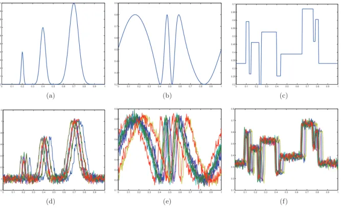
For the mean pattern f to recover, we consider the three test functions shown in Figure 1. Then, for each test function, we simulate n= 20 randomly shifted curves with shifts following a Laplace distributiong(x) = √1
2σexp
−√2|xσ|withσ = 0.1. Gaussian noise is then added to each curve. The level of the additive Gaussian noise is measured as the root of the signal-to-noise ratio (rsnr) defined as rsnr= ! R1 0(f(x)−f¯)2dx ǫ2 %1/2 where f¯= Z 1 0 f(x)dx.
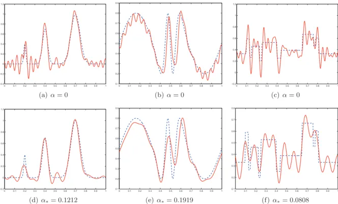
A sub-sample of 10 curves forrsnr= 7is shown in Figure 1 for each test function. The Fourier coefficients of the density g are given by γk = 1+2σ12π2k2 which corresponds to a degree of ill-posednessβ = 2. The condition (2.7) leads to the choicem0 = 32. An example of estimation by spectral cut-off by minimizing the criterion Uα(Y, j) with α = 0 is displayed in Figure 1. One
can see that the obtained estimators are rather oscillatory suggesting that the selected frequency cut-off is somewhat too large when takingα= 0.
These results illustrate the problem of choosing the value of α. To better understand the influence of this parameter, we present a short simulation study. The factors are the number of curves n = 20,50,100 and the signal-to-noise ratio rsnr = 3,7. For each combination of these two factors, we generate m = 1, . . . , M (with M = 100) independent replications of the above described simulations. For each replication m we compute the estimator θ∗α,m for α ranging on a fine grid of [0,1]. Then, since the templatef and its Fourier coefficients θare known, one can compute for each value ofα the following empirical mean squared error (MSE)
M SE(α) = 1 M M X m=1 kθ∗α,m−θk22.
0 0.1 0.2 0.3 0.4 0.5 0.6 0.7 0.8 0.9 1 0 0.1 0.2 0.3 0.4 0.5 0.6 0.7 0.8 0.9 1 (a) 0 0.1 0.2 0.3 0.4 0.5 0.6 0.7 0.8 0.9 1 0.2 0.3 0.4 0.5 0.6 0.7 0.8 0.9 (b) 0 0.1 0.2 0.3 0.4 0.5 0.6 0.7 0.8 0.9 1 0.2 0.25 0.3 0.35 0.4 0.45 0.5 0.55 0.6 0.65 0.7 (c) 0 0.1 0.2 0.3 0.4 0.5 0.6 0.7 0.8 0.9 1 −0.2 0 0.2 0.4 0.6 0.8 1 1.2 (d) 0 0.1 0.2 0.3 0.4 0.5 0.6 0.7 0.8 0.9 1 0.1 0.2 0.3 0.4 0.5 0.6 0.7 0.8 0.9 (e) 0 0.1 0.2 0.3 0.4 0.5 0.6 0.7 0.8 0.9 1 0.1 0.2 0.3 0.4 0.5 0.6 0.7 0.8 (f)
Figure 1: Test functions and an example of randomly shifted curves. First line: (a) Bumps, (b) Sine, (c) Blocks. Second line: sample of 10 curves out ofn= 20for each test function.
For each test function and each combination of the factors, we display in Figure 3 the curve
α → M SE(α). The value α∗ minimizing α → M SE(α) depends on the template to recover.
These simulations show thatα∗ tends to be smaller as the numbernof curves grows. The value of α∗ is also closer to zero when the signal-to-noise ratio decreases (which corresponds to high values of ǫ). This confirms the heuristic arguments developed in Section 2. If the level of noise
ǫis large compared tokθk2
2 (case of a low signal-to-noise ratio), then the model (1.1) is close to the standard white noise deconvolution problem. In this case, settingα= 0leads to satisfactory results which corresponds to taking the classical decomposition of the risk in standard inverse problems to do the estimation.
To conclude this section, let us consider the estimation by spectral cut-off by minimizing the criterion Uα(Y, j) with α = α∗ in the case n = 20 and rsnr = 7. This example is displayed
in Figure 1. One can see that the obtained estimators are much smoother than those obtained with the choice α = 0. This confirms the importance of the choice of α. However, finding a data-based value forα is clearly challenging and is an interesting topic for future work.
Appendix
This Appendix is divided in two parts. In the first part, we detail the scheme used for the proof of Theorem 2.1. The second part contains some technical lemmas. Throughout the proof,
C denote a generic positive constant whose value may change from line to line. We provide first some short definitions which will be used in the sequel. In some sense, these terms measure the complexity associated to the set of filtersΛ using the notations in Cavalieret al. (2002).
Definition 4.1 For each λ∈Λ, define
ρ(λ) = sup |k|≤m0 |γk|−2λk qP |i|≤m0|γi| −4λ4 i , ρΛ= max λ∈Λρ(λ),
0 0.1 0.2 0.3 0.4 0.5 0.6 0.7 0.8 0.9 1 −0.4 −0.2 0 0.2 0.4 0.6 0.8 1 1.2 (a)α= 0 0 0.1 0.2 0.3 0.4 0.5 0.6 0.7 0.8 0.9 1 0.1 0.2 0.3 0.4 0.5 0.6 0.7 0.8 0.9 (b)α= 0 0 0.1 0.2 0.3 0.4 0.5 0.6 0.7 0.8 0.9 1 −0.2 0 0.2 0.4 0.6 0.8 1 1.2 (c) α= 0 0 0.1 0.2 0.3 0.4 0.5 0.6 0.7 0.8 0.9 1 −0.2 0 0.2 0.4 0.6 0.8 1 1.2 (d)α∗= 0.1212 0 0.1 0.2 0.3 0.4 0.5 0.6 0.7 0.8 0.9 1 0.1 0.2 0.3 0.4 0.5 0.6 0.7 0.8 0.9 (e)α∗= 0.1919 0 0.1 0.2 0.3 0.4 0.5 0.6 0.7 0.8 0.9 1 0.1 0.2 0.3 0.4 0.5 0.6 0.7 0.8 (f)α∗= 0.0808
Figure 2: An example of template estimation (n= 20andrsnr= 7) with α= 0and α=α∗ for each test function.
0 0.1 0.2 0.3 0.4 0.5 0.6 0.7 0.8 0.9 1 2 4 6 8 10 12 14 x 10−3 n=20 n=50 n=100 (a) Bumps,rsnr= 7 0 0.1 0.2 0.3 0.4 0.5 0.6 0.7 0.8 0.9 1 2 3 4 5 6 7 8 9 10 x 10−3 n=20 n=50 n=100 (b) Sine,rsnr= 7 0 0.1 0.2 0.3 0.4 0.5 0.6 0.7 0.8 0.9 1 0.004 0.006 0.008 0.01 0.012 0.014 0.016 0.018 0.02 0.022 n=20 n=50 n=100 (c) Blocks,rsnr= 7 0 0.1 0.2 0.3 0.4 0.5 0.6 0.7 0.8 0.9 1 2 4 6 8 10 12 14 x 10−3 n=20 n=50 n=100 (d) Bumps,rsnr= 3 0 0.1 0.2 0.3 0.4 0.5 0.6 0.7 0.8 0.9 1 2 3 4 5 6 7 8 9 10 11 x 10−3 n=20 n=50 n=100 (e) Sine,rsnr= 3 0 0.1 0.2 0.3 0.4 0.5 0.6 0.7 0.8 0.9 1 0 0.005 0.01 0.015 0.02 0.025 n=20 n=50 n=100 (f) Blocks,rsnr= 3
Figure 3: Empirical Mean Square Error (MSE) over M = 100 simulations as a function of
α ∈[0,1] for n= 20,50,100 and rsnr= 7,3 for each test function: Bumps (first column), Sine (second Column), Blocks (third column).
S= max λ∈Λ |isup|≤m0|γi| −2λ2 i min λ∈Λ|isup|≤m0|γi| −2λ2 i , M =X λ∈Λ
For a brief discussion on these quantities, we refer to Cavalier et al. (2002). For all λ∈ Λ, we also introduce Rα(θ, λ)as Rα(θ, λ) = X |k|≤m0 (1−λk)2θ2k+ X |k|≤m0 λ2k|γk|−2+α log2(n) n X |k|≤m0 λ2k|θk|2|γk|−2+ X |k|>m0 |θk|2, (4.2)
which corresponds to an approximation of the quadratic risk. 4.1 Proof of Theorem 2.1
The proof uses the following scheme. The first step consists in computing the quadratic risk of θ⋆ and proving that it is close to R
α(θ, λ⋆). The aim of the second part is to show that
Uα(Y, λ⋆) is close to Rα(θ, λ⋆), even for a random filterλ⋆. Then, we use the fact thatλ⋆
min-imizes the criterion Uα(Y, λ⋆) over the filters in Λ and we compute the expectation of Uα(Y, λ)
for all deterministic λin order to obtain an oracle inequality. Step 1: remark that
Eθkθ⋆−θk2 = EθX k∈Z |θ⋆k−θk|2, = Eθ X |k|≤m0 |λ⋆kγk−1c˜k−θk|2+ X |k|>m0 |θk|2, = Eθ X |k|≤m0 λ⋆k˜γk γk − 1 θk+λ⋆kγ−k1 ǫ √ nξk 2 + X |k|>m0 |θk|2, = Eθ X |k|≤m0 λ ⋆ k ˜ γk γk − 1 2 |θk|2+ ǫ2 nEθ X |k|≤m0 {λ⋆k}2|ξk|2|γk|−2+ X |k|>m0 |θk|2 +2Eθ X |k|≤m0 ǫ √ nRe (λ⋆kγk−1γ˜k−1)θk×λ⋆k¯γk−1ξ¯k ,
where for a given z ∈ C, Re(z) denotes the real part of z and z¯ the conjugate of z. In the following, we denote byR˜(θ, λ) the commonly used risk in inverse problems, i.e.
˜ R(θ, λ) := X |k|≤m0 1−λk ˜ γk γk |θk| 2+ǫ2 n X |k|≤m0 λ2k|γk|−2+ X |k|>m0 |θk|2, ∀λ∈Λ.
ThenEθkθ⋆−θk2 can be rewritten as Eθkθ⋆−θk2 = EθR˜(θ, λ⋆) +ǫ 2 nEθ X |k|≤m0 |γk|−2{λ⋆k}2(|ξk|2−1) +2Eθ X |k|≤m0 ǫ √ nRe (λ ⋆ kγk−1γ˜k−1)θk×λ⋆kγ¯−k1ξ¯k , = EθR˜(θ, λ⋆) +A1+A2. (4.3) In order to bound A1, we follow the notations of Cavalieret al. (2002). Let us define
∆(λ) =LΛ ǫ2 n |ksup|≤m0λ 2 k|γk|−2 and ¯∆(λ) = log2(n) n |ksup|≤m0λ 2 k|γk|−2 for all λ∈Λ, (4.4)
where LΛ has been introduced in (4.1). Then, we apply the inequality (32) of Cavalier et al. (2002): there exists a universal constant C such that for anyγ >0
A1 := ǫ2 nEθ X |k|≤m0 |γk|−2{λ⋆k}2(|ξk|2−1)≤γ ǫ2 nEθ X |k|≤m0 {λ⋆k}2|γk|−2+Cγ−1Eθ∆(λ⋆). (4.5)
Now, consider a bound for A2 defined as A2:= 2Eθ X |k|≤m0 ǫ √ nRe (λ ⋆ kγ−k1˜γk−1)θk×λ⋆k¯γk−1ξ¯k .
We apply inequality(31) of Cavalier et al. (2002) to obtain for anyγ >0
A2 ≤γEθ
X
|k|≤m0
1−λ⋆kγ˜kγk−12|θk|2+Cγ−1Eθ∆(λ⋆). (4.6) Now, for allγ >0, inequalities (4.3), (4.5) and (4.6) yield
Eθkθ⋆−θk2 ≤(1 +γ)EθR˜(θ, λ⋆) +Cγ−1Eθ∆(λ⋆). (4.7) for some positive constant C. At last, we show that R˜(θ, λ⋆) is close to Rα(θ, λ⋆) defined in
(4.2). Remark that EθR˜(θ, λ⋆) = Eθ X |k|≤m0 (1−λ⋆k)2|θk|2+ ǫ2 nEθ X |k|≤m0 {λ⋆k}2|γk|−2+Eθ X |k|>m0 |θk|2 +Eθ X |k|≤m0 |1−λ⋆kγ˜kγk−1|2−(1−λ⋆k)2 |θk|2, = EθR0(θ, λ⋆) +Eθ X |k|≤m0 |θk|2{λ⋆k}2 ˜ γk γk − 1 2 | {z } :=B1 +2Eθ X |k|≤m0 λ⋆k(1−λ⋆k)Re 1− ˜γk γk |θk|2. | {z } :=B2
First, we apply the Lemma 4.1 withK =γ in order to boundB1. We obtain B1 ≤γ log2n n Eθ X |k|≤m0 {λ⋆k}2|γk|−2|θk|2+Ce−γlog 1+τ(n) ,
for someτ >0. ConcerningB2, we use the inequality2ab≤γa+γ−1bfor allγ >0and Lemma 4.1 withK =γ2 in order to obtain
B2 = 2 Eθ X |k|≤m0 λk⋆(1−λ⋆k)Re 1−γk−1γ˜k|θk|2, ≤ γEθ X |k|≤m0 (1−λ⋆k)2|θk|2+γ−1Eθ X |k|≤m0 {λ⋆k}2|θk|2|γk|−2|γk−γ˜k|2, ≤ γEθ X |k|≤m0 (1−λ⋆k)2|θk|2+γ log2(n) n Eθ X |k|≤m0 {λ⋆k}2|θk|2|γk|−2+Ce−γ 2log1+τ(n) .
Therefore, it follows that
EθR˜(θ, λ⋆) ≤ (1 +γ)EθR0(θ, λ⋆) + 2γlog 2(n) n Eθ X |k|≤m0 {λ⋆k}2|θk|2|γk|−2+Ce−γ 2log1+τ(n) , ≤ (1 + 2γ)EθRα(θ, λ⋆) + (1−α)γkθk2Eθ∆(¯ λ⋆) +Ce−γ2log1+τ(n). Using (4.7), we get Eθkθ⋆−θk2 ≤(1 + 2γ)2EθRα(θ, λ⋆) +Cγ−1Eθ∆(λ⋆) +C(1−α)γkθk2Eθ∆(¯ λ⋆) +Ce−γ2log1+τ(n). (4.8)
This concludes the Step 1.
Step 2: First, we write Uα(Y, λ⋆)in terms of Rα(θ, λ⋆). Remark that
Uα(Y, λ⋆) = X |k|≤m0 ({λ⋆k}2−2λ⋆k)|γk|−2 |˜ck|2− ǫ2 n + ǫ 2 n X |k|≤m0 {λ⋆k}2|γk|−2 +αlog 2(n) n X |k|≤m0 {λ⋆k}2|γk|−4 |˜ck| − ǫ2 n , = Rα(θ, λ⋆) + X |k|≤m0 ({λ⋆k}2−2λ⋆k)|γk|−2 |c˜k|2− ǫ2 n −(1−λ⋆k)2θk2 − X |k|≥m0 |θk|2+α log2(n) n X |k|≤m0 {λ⋆k}2 |γk|−4 |c˜k| − ǫ2 n − |γk|−2|θk|2 . (4.9)
Recall that for all k∈N
|˜ck|2 =|θk˜γk|2+ ǫ2 n|ξk| 2+ 2√ǫ nRe(θkγ˜kξ¯k), and |γk|−2|c˜k|2=|θk|2 ˜ γk γk 2 + ǫ 2 n|γk| −2|ξ k|2+ 2 ǫ √ n|γk| −2Re(θ k˜γkξ¯k).
Hence, equality (4.9) can be rewritten as
Rα(θ, λ⋆) = Uα(Y, λ⋆) +kθk2+ X |k|≤m0 (2λ⋆k− {λ⋆k}2)θk2 ! ˜ γk γk 2 −1 % +ǫ 2 n X |k|≤m0 (2λ⋆k− {λ⋆k}2)|γk|−2(|ξk|2−1) +2√ǫ n X |k|≤m0 (2λ⋆k− {λ⋆k}2)|γk|−2Re(˜γkθkξ¯k) +αlog 2(n) n X |k|≤m0 {λ⋆k}2 |γk|−2|θk|2− |γk|−4 |c˜k|2− ǫ2 n , = Uα(Y, λ⋆) +kθk2+C1+C2+C3+C4. (4.10) First consider the bound of C1. Thanks to Lemma 4.2
C1 := X |k|≤m0 (2λ⋆k− {λ⋆k}2)θk2 ! ˜ γk γk 2 −1 % , ≤ γEθRα(θ, λ⋆) + γ+ γ− 1 log2(n) Rα(θ, λ0) + (1−α)γkθk2Eθ∆(λ⋆) +(1−α)γ−1kθk2∆(¯ λ0) +Ce−γ2log1+τ(n).
Concerning C2, we use the inequality (36) of Cavalieret al. (2002). We get C2 := ǫ2 n X |k|≤m0 (2λ⋆k− {λ⋆k}2)|γk|−2(|ξk|2−1), ≤ 2γǫ 2 n X |k|≤m0 {λ⋆k}2|γk|−2+Cγ−1Eθ∆(λ⋆). (4.11)
Then, using Lemma 4.3 C3 := ǫ √ n X |k|≤m0 (2λ⋆k− {λ⋆k}2)|γk|−2Re(˜γkθkξ¯k) ≤ 3γEθR(θ, λ⋆) + 2γR(λ0, θ) +Cγ−1Eθ∆(λ⋆) +Cγ−1Eθ∆(λ0). (4.12) We are now interested in C4, the last residual term of (4.10). Thanks to the definition of˜ck:
C4 := log2n n Eθ X |k|≤m0 {λ⋆k}2|γk|−2 −|γk|−2|˜ck|2+ ǫ2 n|γk|− 2+|θ k|2 = log 2n n Eθ X |k|≤m0 {λ⋆k}2|γk|−2|θk|2 ! 1− ˜ γk γk 2% +ǫ 2 n log2n n Eθ X |k|≤m0 {λ⋆k}2|γk|−4(1− |ξk|2) −2log 2n n ǫ √ nEθ X |k|≤m0 {λ⋆k}2|γk|−4Re(θkγ˜kξ¯k), ≤ DγEθRα(θ, λ⋆) +DγRα(θ, λ0) +(1−α)γkθk2Eθ∆(λ⋆) + (1−α)γ−1kθk2∆(¯ λ0) +Ce−log1+τ(n), (4.13) for some D, C >0 independent ofǫ and n. Indeed, we can use essentially the same algebra as for the bound of the terms C1, C2 and C3 and the inequality
|γk|−2≤
n
log2n, ∀k≤m0.
Now, we are interested in the terms∆(.) and∆(¯ .)introduced in (4.4). For all λ∈Λ andx >0, we have sup |k|≤m0 λ2k|γk|−2 ≤ 1 x X |k|≤m0 λ2k|γk|−2+ sup |k|≤m0 λ2k|γk|−21n xsup|k|≤m0λ 2 k|γk|−2≥P|k|≤m0λ 2 k|γk|−2 o ≤ 1 x X |k|≤m0 λ2k|γk|−2+ω(x), (4.14)
where the function ω is introduced in Theorem 2.1. Hence, using (4.10)-(4.14) with a suitable choice forx, (1−Dγ)EθRα(θ, λ⋆) ≤ EθUα(Y, λ⋆) +kθk2+D γ+ γ− 1 log2(n) Rα(θ, λ0) +Ce−log 1+τ(n) +C1 ǫ2 nLΛω (1−α)kθk 2L Λγ−1+C2 log2n n ω (1−α)kθk 2log2(n)γ−1
Step 3: From the definition of λ⋆, we immediately get (1−Dγ)EθRα(θ, λ⋆) ≤ EθUα(Y, λ0) +kθk2+D γ+ γ− 1 log2(n) Rα(θ, λ0) +Ce−log 1+τ(n) +C1 ǫ2 nLΛω (1−α)kθk 2L Λγ−1+C2 log2n n ω (1−α)kθk 2log2(n)γ−1,
where λ0 denotes the oracle bandwidth. Step 4: Using that for all |k| ≤m0,Eθ
ˆ Θ2k= |θk|2 1− 1 n+nγ12 k ≤ |θk|2 1− 1 n +log21(n) it follows that EθUα(Y, λ0)≤ 1 + 1 log2(n) Rα(θ, λ0)− kθk2 .
4.2 Technical Lemmas
Lemma 4.1 For all K >0, we have Eθ X |k|≤m0 {λ⋆k}2 ˜ γk γk − 1 2 |θk|2 ≤K log2(n) n Eθ X |k|≤m0 {λ⋆k}2|γk|−2|θk|2+Ce−Klog 1+τ(n) ,
where C, τ denote positive constants independent of ǫand n.
PROOF. Let Q >0 a deterministic term which will be chosen later. Eθ X |k|≤m0 {λ⋆k}2 ˜ γk γk − 1 2 |θk|2 =Eθ X |k|≤m0 {λ⋆k}2|θk|2|γk|−2|˜γk−γk|2, ≤ QEθ X |k|≤m0 {λ⋆k}2|θk|2|γk|−2+Eθ X |k|≤m0 {λ⋆k}2|θk|2|γk|−2 |˜γk−γk|2−Q 11{|˜γk−γk|2>Q}. Thanks to (2.7) and the monotonicity of λ, we have
Eθ X |k|≤m0 {λ⋆k}2|θk|2|γk|−2 |˜γk−γk|2−Q 11{|˜γk−γk|2>Q} ≤ C n log2(n) X |k|≤m0 |θk|2Eθ |˜γk−γk|2−Q 11{|˜γk−γk|2>Q}. For all |k| ≤m0, using an integration by part
Eθ|˜γk−γk|2−Q11
{|γ˜k−γk|2>Q}=
Z +∞
Q
P(|γ˜k−γk|2 ≥x)dx.
Letx≥Q. A Bernstein type inequality provides
P(|˜γk−γk|2 ≥x) = P ! 1 n n X l=1 n e−2iπkτl−E[e−2iπkτl] o ≥ √ x % , ≤ 2 exp − (n √ x)2 2Pnl=1Var(e−2iπkτl) +n√x/3 , ≤ 2 exp − n 2x 2n+n√x/3 .
Hence, for all|k| ≤m0,
Eθ|˜γk−γk|2−Q11 {|γ˜k−γk|2>Q} ≤ Z +∞ Q exp − nx 2 +√x/3 dx, ≤ Z 36 Q expn−nx 4 o dx+ Z +∞ 36 exp−Cn√x dx≤ C ne −Qn/4,
where C denotes a positive constant independent of Q. Let K > 0. Choosing for instance
Q=n−1Klog2(n), we obtain Eθ X |k|≤m0 {λ⋆k}2 ˜ γk γk − 1 2 |θk|2 ≤ K log2(n) n Eθ X |k|≤m0 {λ⋆k}2|γk|−2|θk|2+C nm0 log2(n)e −Klog2 (n)/4, ≤ Klog 2(n) n Eθ X |k|≤|m0| {λ⋆k}2|γk|−2|θk|2+Ce−Klog 1+τ(n) ,
Lemma 4.2 Let λ⋆ defined in (2.13). For all deterministic filter λand 0< γ <1, we have
Eθ X |k|≤m0 |θk|2{λ⋆k}2 ! ˜ γk γk 2 −1 % ≤ γEθRα(θ, λ⋆) + γ+ γ− 1 log2(n) Rα(θ, λ0) +(1−α)γ−1kθk2∆(¯ λ0) + (1−α)γkθk2Eθ∆(¯ λ⋆) +Ce−γ2log1+τ(n). where C, τ denote positive constants independent of ǫand n.
PROOF. First, remark that Eθ X |k|≤m0 |θk|2{λ⋆k}2 ! ˜ γk γk 2 −1 % = Eθ X |k|≤m0 |θk|2{λ⋆k}2|γk|−2(|γ˜k−γk+γk|2− |γk|2), = Eθ X |k|≤m0 |θk|2{λ⋆k}2|γk|−2|˜γk−γk|2 +2Eθ X |k|≤m0 |θk|2{λ⋆k}2|γk|−2Re((˜γk−γk)¯γk) (4.15)
Letλ∈Λ be a deterministic filter, sinceEθγ˜k=γk for allk∈N, we can write that Eθ X |k|≤m0 |θk|2{λ⋆k}2|γk|−2Re((˜γk−γk)¯γk) =Eθ X |k|≤m0 |θk|2({λ⋆k}2−λ2k)|γk|−2Re((˜γk−γk)¯γk),
and simple algebra yields
|{λ⋆k}2−λ2k| ≤λ⋆k|1−λ⋆k|+λk|1−λk|+λ⋆k|1−λk|+λk|1−λ⋆k|,∀k∈N.
Next, the Young inequality implies that for allγ ∈]0; 1]: Eθ X |k|≤m0 |θk|2 {λ⋆k}2−λ2k|γk|−2Re((˜γk−γk)¯γk) (4.16) ≤ γ−1 X |k|≤m0 [{λ⋆k}2+{λk}2 |θk|2|γk|−2|γ˜k−γk|2+γ X |k|≤m0 |1−λk|2+|1−λ⋆k|2 |θk|2.
Hence, from equations (4.15) and (4.16), we obtain Eθ X |k|≤m0 |θk|2{λ⋆k}2 ! ˜ γk γk 2 −1 % ≤ (1 +γ−1)Eθ X |k|≤m0 |θk|2{λ⋆k}2|γk|−2|˜γk−γk|2+γ−1Eθ X |k|≤m0 |θk|2λ2k|γk|−2|γ˜k−γk|2 +γEθ X |k|≤m0 |1−λk|2+|1−λ⋆k|2 |θk|2.
A direct application of Lemma 4.1 provides, for all K >0 Eθ X |k|≤m0 |θk|2 ! ˜ γk γk 2 −1 % ≤ (1 +γ−1)Klog 2(n) n Eθ X |k|≤m0 |θk|2{λ⋆k}2|γk|−2+ γ−1 n X |k|≤m0 λ2k|θk|2|γk|−2(1− |γk|2) +2γEθ X |k|≤m0 [|1−λk|2+|1−λk⋆|2]|θk|2+Ce−Klog 1+τ(n) .
FixK =γ2 and remark that X |k|≤m0 |γk|−2|θk|2λ2k≤ kθk2 sup |k|≤m0 λ2k|γk|−2,∀λ∈Λ,
in order to conclude the proof of Lemma 4.2.
Lemma 4.3 Let λ⋆ the filter defined in (2.13). For all deterministic filter λand 0< γ <1, we have 2ǫ √ nEθ X |k|≤m0 2λ⋆k− {λ⋆k}2|γk|−2Re(θk˜γkξ¯k)≤2γR(θ, λ) +3γEθR(θ, λ⋆) +Cγ−1Eθ∆(λ⋆) +Cγ−1Eθ∆(λ) +Ce−log1+τ(n), for someτ >0.
PROOF. In the following, we first state the inequality
P !m0 \ k=1 ˜ γk γk ≤2 % ≥1−Cm0exp(−log2n), for some τ >0. Indeed
P !m0 [ k=1 ˜ γk γk >2 % ≤ m0 X k=1 P ˜ γk γk >2 ≤ m0 X k=1 P(|˜γk−γk|>|γk|), ≤ m0 X k=1 P |γ˜k−γk|> log2(n) n , ≤ Cm0exp(−log2n).
Then, for allγ >0, using the above result and inequality (35) of Cavalieret al. (2002), we obtain 2ǫ √ nEθ X |k|≤m0 2λ⋆k− {λ⋆k}2|γk|−2Re(θk˜γkξ¯k) ≤ γ X |k|≤m0 (1−λk)2|θk|2+ ǫ2 nEθ X |k|≤m0 λ2k|γk|−4|γ˜k|2 +γEθ X |k|≤m0 (1−λ⋆k)2|θk|2+ ǫ2 n X |k|≤m0 {λ⋆k}2|γk|−4|˜γk|2 +Cγ−1Eθ∆(λ⋆) +Cγ−1Eθ∆(λ), ≤ 4γ X |k|≤m0 (1−λk)2|θk|2+ ǫ2 nEθ X |k|≤m0 λ2k|γk|−2 +Ce−log1+τ(n) +4γEθ X |k|≤m0 (1−λ⋆k)2|θk|2+ ǫ2 n X |k|≤m0 {λ⋆k}2|γk|−2 +Cγ−1Eθ∆(λ⋆) +Cγ−1Eθ∆(λ). This concludes the proof.
References
Bigot, J. (2006). Landmark-based registration of curves via the continuous wavelet transform. Journal of Computational and Graphical Statistics,15(3), 542-564.
Bigot, J. and Gadat, S. (2010). A deconvolution approach to estimation of a common shape in a shifted curves model. Annals of statistics,to be published.
Bigot, J., Gamboa, F. and Vimond, M. (2009). Estimation of translation, rotation and scal-ing between noisy images usscal-ing the fourier mellin transform. SIAM Journal on Imaging Sciences, 2, 614-645.
Brown, L. D. and Low, M. G. (1996). Asymptotic equivalence of nonparametric regression and white noise. Ann. Statist.,24(6), 2384–2398.
Castillo, I. and Loubes, J.-M. (2009). Estimation of the distribution of random shifts deformation. Math. Methods Statist.,18(1), 21–42.
Cavalier, L., Golubev, G. K., Picard, D. and Tsybakov, A. B. (2002). Oracle inequalities for inverse problems. Ann. Statist., 30(3), 843–874. (Dedicated to the memory of Lucien Le Cam)
Cavalier, L. and Hengartner, N. W. (2005). Adaptive estimation for inverse problems with noisy operators. Inverse Problems,21(4), 1345–1361.
Cavalier, L. and Raimondo, M. (2007). Wavelet deconvolution with noisy eigenvalues. IEEE Trans. on Signal Processing, 55, 2414–2424.
Dalalyan, A. (2007). Penalized maximum likelihood and semiparametric second-order efficiency. Math. Methods of Statist.,16(1), 43-63.
Dalalyan, A., Golubev, G. and Tsybakov, A. B. (2006). Penalized maximum likelihood and semiparametric second-order efficiency. Ann. Statist.,34(1), 169-201.
Donoho, D. L. (1995). Nonlinear solution of linear inverse problems by wavelet-vaguelette decomposition. Appl. Comput. Harmon. Anal.,2(2), 101–126.
Donoho, D. L., Johnstone, I. M., Kerkyacharian, G. and Picard, D. (1995). Wavelet shrinkage: Asymptopia? J. Roy. Statist. Soc. Ser. B,57, 301–369.
Efromovich, S. and Koltchinskii, V. (2001). On inverse problems with unknown operators. IEEE Transactions on Information Theory,47(7), 2876-2894.
Fan, J. (1991). On the optimal rates of convergence for nonparametric deconvolution problems. Ann. Statist.,19, 1257–1272.
Gamboa, F., Loubes, J.-M. and Maza, E. (2007). Semi-parametric estimation of shifts. Electron. J. Stat.,1, 616–640.
Gasser, T. and Kneip, A. (1992). Statistical tools to analyze data representing a sample of curves. Ann. Statist.,20(3), 1266-1305.
Gasser, T. and Kneip, A. (1995). Searching for structure in curve samples. JASA, 90(432), 1179-1188.
Hoffmann, M. and Reiß, M. (2008). Nonlinear estimation for linear inverse problems with error in the operator. Annals of Statistics,38, 310-336.
Isserles, U., Ritov, Y. and Trigano, T. (2008). Semiparametric density estimation of shifts between curves. preprint.
Kneip, A. and Gasser, T. (1988). Convergence and consistency results for self-modelling regres-sion. Ann. Statist.,16, 82-112.
Liu, X. and Müller, H. (2004). Functional convex averaging and synchronization for time-warped random curves. JASA,99(467), 687-699.
Marteau, C. (2006). Regularization of inverse problems with unknown operator. Mathematical Methods of Statistics,15, 415-443.
Marteau, C. (2009). On the stability of the risk hull method for projection estimator. Journal of Statistical Planning and Inference,139, 1821-1835.
Ramsay, J. and Li, X. (2001). Curve registration. Journal of the Royal Statistical Society, Series B,63, 243-259.
Ramsay, J. and Silverman, B. (2002). Functional data analysis. New York: Spriner-Verlag: Lecture Notes in Statistics.
Ramsay, J. and Silverman, B. (2005). Applied functional data analysis. New York: Spriner-Verlag: Lecture Notes in Statistics.
Ronn, B. B. (1998). Nonparametric maximum likelihood estimation for shifted curves. JRSS B, 60, 351-363.
Vimond, M. (2010). Efficient estimation for a subclass of shape invariant models. Annals of statistics,38(3), 1885-1912.
Wang, K. and Gasser, T. (1997). Alignment of curves by dynamic time warping. Ann. Statist., 25(3), 1251-1276.