Semi-parametric Bayesian Inference of Accelerated Life Test Using Dirichlet Process Mixture Model

Mixture Model

A dissertation presented to the faculty of

the Russ College of Engineering and Technology of Ohio University

In partial fulfillment of the requirements for the degree

Doctor of Philosophy

Xi Liu December 2015

This dissertation titled

Semi-parametric Bayesian Inference of Accelerated Life Test Using Dirichlet Process Mixture Model

by XI LIU

has been approved for

the Department of Industrial and Systems Engineering and the Russ College of Engineering and Technology by

Tao Yuan

Associate Professor of Industrial and Systems Engineering

Dennis Irwin

ABSTRACT

LIU, XI, Ph.D., December 2015, Mechanical and Systems Engineering

Semi-parametric Bayesian Inference of Accelerated Life Test Using Dirichlet Process Mixture Model (100 pp.)

Director of Dissertation: Tao Yuan

Accelerated life testing (ALT) is commonly used to estimate the reliability of highly reliable products. This dissertation develops statistical models to predict useful life of nano devices with data collected under constant-stress ALT and step-stress ALT. As an example of nano devices, nc-MoOx embedded ZrHfO high-k dielectric thin film is studied with respect to its physical properties, failure mechanisms, and long-term stability. The devices used for ALT and reliability prediction demonstration have identical structure with this nc-MoOx embedded device.

This research develops a semi-parametric Bayesian method to analyze ALT. The model assumes a log-linear lifetime-stress relationship, without assuming any parametric form of the failure-time distribution. The Dirichlet Weibull mixture model is employed to model the failure-time distribution under a given stress level. The model is fitted with a simulation-based algorithm, which implements Gibbs sampling to analyze ALT data and predicts the failure-time distribution at a normal stress level.

Two practical examples related to the reliability of nanoelectronic devices are presented for constant-stress ALT, including one right-censored data and one complete data set. One right-censored practical example is demonstrated for simple step-stress

ALT. All three examples illustrate the capability of the proposed methodology to provide accurate prediction of the failure-time distribution at a normal stress level.

DEDICATION

This dissertation is dedicated to my dear father, Jianzhen Liu, and to my mother, Jinping Deng.

ACKNOWLEDGMENTS

Over the past five years of doctoral journey, I have received numerous encouragement and support from a great number of persons and institutions. My work cannot be completed without their support.

First and foremost, I would like to express my deepest appreciation to my advisor, Dr. Tao Yuan, for his continuous support and guidance throughout my graduate studies. I would never have been able to finish this dissertation without his persistent help and deep knowledge. I also would like to thank Dr. Yue Kuo, who has offered me the great opportunity to do tests in Thin Film Nano & Microelectronics Research Laboratory, Texas A&M University, for his support on this dissertation and for guiding me to the semiconductor devices’ field.

Next, I would like to thank Dr. Andrew Snow, Dr. David Koonce and Dr. Diana Schwercha, for serving my committee members and offering many insightful comments and suggestions to my research.

I am deeply grateful to Dr. Chia-Han Yang and Dr. Chi-Chou Lin for fabricating samples, teaching me the device concepts and mentoring me on testing and measurements. Thanks Minghao Zhu for the XPS and XRD analyzes. Thanks Dr. Saleem Z. Ramadan and Dr. Wen Luo for supplying me data sets as my practical examples.

Lastly, I would like to thank my family, for their continuous support, inspiration and love.

This dissertation was partially supported by National Science Foundation project CMMI-0926420 and CMMI-0926379.

TABLE OF CONTENTS Page Abstract ... 3 Dedication ... 5 Acknowledgments... 6 List of Tables ... 9 List of Figures ... 10 Chapter 1: Introduction ... 11

1.1 Motivation and Objective ... 11

1.2 Reliability and Related Functions ... 12

1.3 Accelerated Life Testing ... 14

1.4 Acceleration Model ... 16

1.5 Step-Stress Accelerated Life Testing ... 17

1.6 Commonly Used Estimation Method ... 19

1.6.1 Parametric method ... 20

1.6.2 Nonparametric Bayesian method ... 22

1.6.3 Dirichlet process mixture model ... 24

1.7 Nanocrystals Embedded High-k Device ... 27

1.8 Dissertation Overview ... 28

Chapter 2: Literature Review ... 29

2.1 Inference of Constant-Stress Accelerated Life Testing ... 29

2.1.1 Parametric estimation of constant-stress ALT ... 29

2.1.2 Semi-parametric estimation of constant-stress ALT ... 33

2.2 Inference of Step-Stress Accelerated Life Testing ... 36

2.2.1 Parametric estimation of step-stress accelerated life testing ... 36

2.2.2 Semi-parametric estimation of step-stress accelerated life testing ... 40

2.3 Dirichlet Process Mixture Model ... 41

Chapter 3: Problem Statement ... 44

3.1 Notations ... 44

3.3 Problem Description ... 45

3.3.1 Investigation of metal oxide nanodots-embedded ZrHfO high-k film ... 46

3.3.2 Development of simulation-based algorithm ... 46

3.3.3 Comparison between parametric Weibull log-linear ALT model and DP Weibull mixture ALT model ... 46

Chapter 4: Memory Functions of Molybdenum Oxide Nanodots Embedded ZrHfO High-k† _{... 47}

4.1 Fabrication of Nanocrystals Embedded ZrHfO High-k Device ... 47

4.2 Physical Properties of Nanocrystals Embedded ZrHfO high-k Device ... 48

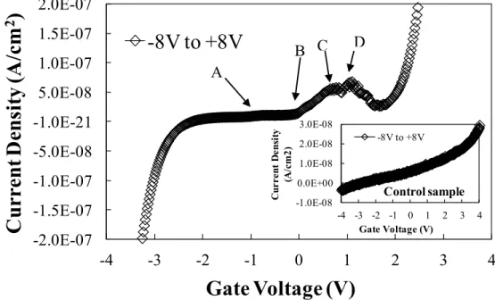
4.3 Charge Trapping and Detrapping Mechanisms ... 49

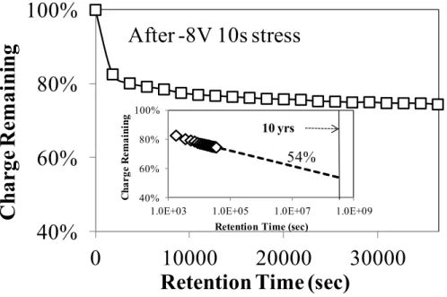
4.4 Charge Retention Capability ... 53

4.5 Conclusions ... 54

Chapter 5: Bayesian Analysis For Accelerated Life tests Using Dirichlet Process Weibull Mixture Model† ... 56

5.1 Methodologies ... 56

5.1.1 Dirichlet process Weibull mixture ALT model ... 56

5.1.2 Simulation-based model fitting ... 60

5.2 Illustrative Examples ... 69

5.2.1 Complete data set example ... 70

5.2.2 Right-censored data set example ... 74

5.3 Conclusions ... 76

Chapter 6: Bayesian Analysis For Simple Step-Stress Accelerated Life Testing ... 78

6.1 Methodologies ... 78

6.2 Illustrative Examples ... 81

Chapter 7: Conclusions ... 84

7.1 Memory Functions of MoOx Nanodots Embedded ZrHfO High-k ... 84

7.2 Prediction of CDF of Failure-Time Distribution at Normal Stress Level ... 84

7.3 Future Research ... 85

LIST OF TABLES

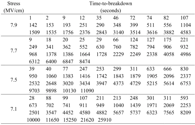
Page Table 5.1: Example 1: times-to-breakdown of MOS capacitors tested at four electrical

field stresses ...70 Table 5.2: Example 2: times-to-breakdown of nanocrystals-embedded high-k memories

tested at four voltage stresses ...75 Table 6.1: Times-to-breakdown of nanocrystals-embedded high-k memories under simple

LIST OF FIGURES

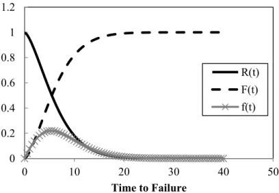
Page Figure 1.1: The reliability function, CDF and PDF of the Weibull distribution with= 1.5

and= 7 ...13

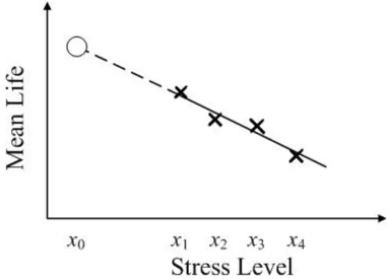
Figure 1.2: Accelerated life testing concept ...15

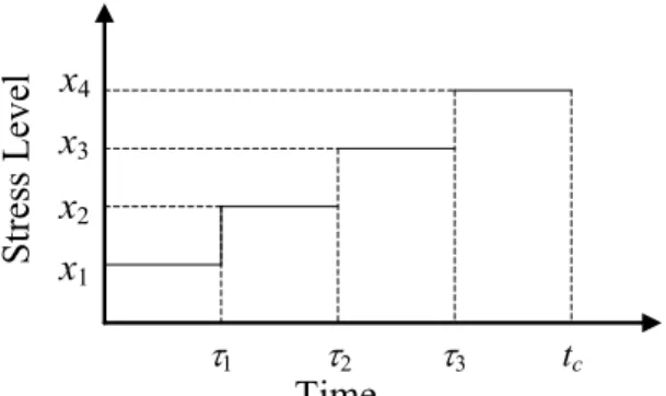
Figure 1.3: Step-stress accelerated life testing ...18

Figure 1.4: Cross-sectional view of nanocrystals embedded ZrHfO capacitor ...28

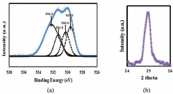
Figure 4.1: (a) XPS O 1s peak, and (b) XRD pattern of the MoOx embedded ZrHfO sample ...49

Figure 4.2: C-V hysteresis curves of the nc-MoOx embedded ZrHfO capacitor measured at 1MHz. The inset is the hysteresis curve of the control sample ...51

Figure 4.3: J-V curve of nc-MoOx embedded capacitor Vg swept from -8 V to +8 V. The inset is the J-V curve of control sample ...52

Figure 4.4: Retention property of holes trapped in the nc-MoOx embedded capacitor. The inset shows the extrapolation of the curve to 10 years projection. ...54

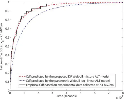
Figure 5.1: Example 1: predicted failure-time CDF at the normal stress x0 = 7.1MV/cm ...72

Figure 5.2: Example 1: estimation of failure-time CDF at 7.9 MV/cm ...74

Figure 5.3: Example 2: predicted failure-time CDF at the normal stress x0 = 7.1 V ...76

Figure 6.1: Trace plots of *, , and * ...82

CHAPTER 1: INTRODUCTION 1.1 Motivation and Objective

For the purpose of increasing competitive advantages, decreasing costs, and satisfying increasing customer expectations, manufacturers strive to design and produce highly reliable products. Consequently, the studies of reliability data analysis have been promoted. Quantitative methods to predict and assess product reliability are required to improve reliability of existing products and ensure the high reliability of new products [1]. The data obtained from life tests are commonly supplied to statistical method for reliability estimation [2]. Conventional lifetime data analysis assumes the failure time following certain parametric distributions such as exponential, Weibull, or log-normal and estimates the parameters of the distributions [3]. However, in some situations it may be difficult to choose the appropriate parametric model. For example, modern complex products may involve multiple failure modes and therefore simple lifetime distributions are not adequate to describe their failure mechanisms. For some new technologies such as nanotechnology, the failure mechanisms have not been well understood. Therefore, more flexible nonparametric methods are needed. In recent years, the development of Markov chain Monte Carlo (MCMC) methods for simulation-based implementation and analysis assures the feasibility of nonparametric data analysis [4].

This dissertation aims to assess the reliability under normal stress levels based on ALT using Bayesian models involving Dirichlet process mixture Models (DPMM). Both constant-stress ALT and step-stress ALT are studied in this work. The rest of this chapter

provides a brief background introduction of reliability and related functions, ALT, acceleration models, step-stress ALT, and commonly used estimation methods.

1.2 Reliability and Related Functions

The reliability is the probability that a system or component can perform its function under operation conditions for a specified period of time. It can be mathematically presented as:

R(t) = Pr{T ≥ t}, (1.1) where T is a random variable denoting the time to failure of a non-repairable device or the time to the first failure of a repairable device, and R(t) is called the reliability function of the failure-time distribution.

Denote F(t) as the cumulative distribution function (CDF) of the failure-time distribution, which is the probability that the lifetime is less than t, i.e.,

F(t)= 1-R(t) = Pr{T <t}. (1.2) If the CDF is a continuous function of t, a third function defined by the derivative of F(t) is used to describe the shape of the failure-time distribution. It is called the probability density function (PDF), and can be expressed as:

( ) ( ) ( ), dt t dR dt t dF t f   (1.3) where f(t) is a non-negative function.

Taking Weibull failure-time distribution as an example, its PDF, CDF, and reliability function can be written as:

             t t t f() 1exp _{, (1.4)}

, 1 exp ) ( / 0 1        t t e dt t t t F  _{ }       _ 

_

Figure 1.1 graphically shows these three functions when the time to failure follows the Weibull distribution with the shape parameter = 1.5 and the scale parameter = 7.

Figure 1.1. The reliability function, CDF and PDF of the Weibull distribution with= 1.5 and= 7.

Another important function, the failure rate or hazard rate function, is used to provide an instantaneous failure rate, which can be denoted as:

. ) ( ) ( } Pr{ ) ( ) ( lim ) ( 0 R t t f t T t t F t t F t h _t          (1.7) 0 0.2 0.4 0.6 0.8 1 1.2 0 10 20 30 40 50 Time to Failure R(t) F(t) f(t)

When h(t) is an increasing, constant, or decreasing function, the failure rate can be described as increasing (IFR), constant (CFR), or decreasing (DFR), respectively [5].

The mean time to failure (MTTF) and the median time to failure are commonly used as measures of the center of a failure-time distribution. The MTTF is the average length of time until failure, and can be defined as the expected value of T, i.e.,

MTTFE(T)





F(tp) = p, (1.9) then tp is called the pth percentile of the lifetime distribution, which means 100p% of the failures occur before time tp. If p=0.5, then t0.5 is the median time to failure. When the distribution is highly skewed, the median is preferentially used as the measure of the center location of a distribution. The median, t0.5, as well as the lower and upper 25% percentiles, t0.25 and t0.75, respectively, are important characteristics of a lifetime distribution.

1.3 Accelerated Life Testing

Reliability life testing is carried out to obtain failure information for the purpose of quantifying reliability [5]. Highly reliable products, such as electronic devices, usually have long lifetimes. Therefore, only very few failures can be obtained within reasonable time period under actual operating condition and it is difficult to obtain adequate failure-time data for statistical methods. One approach to solve this problem is to use ALT, in which the units are placed under higher than operational stress conditions to speed up the failure occurrence [2]. Classical stress includes voltage, current, humidity, temperature,

pressure, cycling rate or load [6]. Then the failure-time data collected at elevated stress levels are analyzed and extrapolated to predict the reliability at the normal stress level through an acceleration model. ALT is based on the fundamental principles that the unit under test will have the same failure mechanisms in a short time at a high stress level as it exhibits in a longer time at a lower stress level [7]. Figure 1.2 shows the basic concept of an ALT estimation which uses lifetime data collected from a four-level single-stress test to estimate mean life under normal stress. The variable xi denotes the stress level with x0 representing the normal stress. According to Dasgupta and Pecht [8], there are four categories of failure mechanisms: stress-strength, damage-endurance, challenge-response, and tolerance-requirement. The ALT is the most appropriate with the damage-endurance failure and some cases of tolerance-requirement failure [7].

Figure 1.2. Accelerated life testing concept.

The constant-stress ALT and the step-stress ALT are the two typical types of accelerated life testing. In constant-stress ALT each single unit is placed only under one

higher than normal stress level, while the step-stress ALT (SSALT) allows several stress levels.

1.4 Acceleration Model

One difficulty of ALT data analysis is how to predict the reliabilities of units at the normal stress level from the failure-time data under higher stress levels. Basically, a functional relationship called the acceleration function is applied to describe the relationship between the lifetimes and the stress conditions [6]. The log-linear model which assumes the log-linear relation for the lifetime is widely used, it can be expressed as: m mx b x b a    ... ln 1 1 , (1.10)

where denotes the stress related characteristic, and x1,…,xm denote the stress factors (or proper transformation of them). The log-linear model is used because it is simple and can be transformed from many other relationships.

For example, when the temperature primarily contributes to the failures, the Arrhenius model is commonly used:

, exp        KT E A r a _(1.11)

where r is the reaction or process rate, A is constant, Ea represents the activation energy in electron volts, T is the absolute temperature(˚K), and K is the Boltzmann’s constant, a known physical constant equals to 8.617×10-5 (eV/˚K) [9]. This equation can be transformed to the log-linear model as lnr = lnA-(Ea/K) (1/T) with x=1/T.

The generalized Eyring model is applicable for failures related to two types of stresses, one thermal and one nonthermal stress. The simplest form of Eyring model can be presented as: , ) ( exp exp               s T C B KT E AT r  a _(1.12)

where r is the process rate, A, , B, and C are constants, Ea is the activation energy, T is the absolute temperature(˚K), K is the Boltzmann’s constant, and s is the second stress [10]. When =0 and C=0, this equation can be transformed to the log-linear model as

Bs T K E A r ln ( a/ )(1/ ) ln with x1=1/T and x2=s.

The E-model can be used to study the time-dependent dielectric breakdown of gate dielectric thin films where the stress is the electrical field. The E-model is expressed as:

 _Lexp





In this study, the log-linear acceleration model will be used and the details will be introduced in section 5.1.1.

1.5 Step-Stress Accelerated Life Testing

Step-stress accelerated life testing (SSALT) can further ensure enough failures within reasonable time period by testing the units through more than one level of stress. In the SSALT, the stress levels change (usually increase) at pre-specified times (time-step

stress ALT) or after pre-specified numbers of failures (failure-step stress ALT). A test with only one change of stress is called a simple step-stress ALT, while a test with several stress changes is called a multiple step-stress ALT [6]. The number of failures in the time-step stress ALT is random at each level of stress. The time duration of each level of stress in the failure-step stress ALT is also random. If the test ends at a pre-specified time, it is called type-I censoring; if the test ends when a pre-specified number of failures has achieved, it is called type-II censoring. Figure 1.3 shows a multi-SSALT with four stresses and type-I censoring. The test ends at a pre-specified time tc. All units that have not failed by tc are censored. The xi’s and i’s are the stress levels and stress changing times, respectively.

In order to analyze SSALT data, a model describing the effect of changing stress is needed. Nelson [12] proposed the cumulative exposure model, which assumes that “the remaining life of specimens depends only on the current cumulative fraction failed and current stress- regardless of how the fraction accumulated.”

Time Stress Leve l x1 x2 1 tc x3 x4 2 3

Denote Fi as the CDF of the failure-time distribution under stress xi, Fi under a step-stress pattern expressed by the cumulative exposure model can be written as:

                       , ), ( ... ... , ), ( , ), ( , 0 ), ( ) ( 3 2 2 2 3 2 1 1 1 2 1 1 0 t t F t u t F t u t F t t F t F m m         (1.14)

where τi is the time of changing the stress from the ith stress level to the (i+1)th stress level, Fi(t) is the CDF under the ith stress level, and ui is the solution of

Fi+1(ui) =Fi(τi- τi-1 + ui-1).

This dissertation studies the simple SSALT with two stress levels and assumes the failure-time distribution under each stress level following a Dirichlet process mixture model with Weibull kernel. The details of inference will be given in Chapter 6.

1.6 Commonly Used Estimation Method

The commonly used data estimation method for ALT analysis can be classified as parametrical and non-parametrical, depending on if there are parameters assumed in the model. Two widely applied parametric estimation groups are Maximum Likelihood Estimation and parametrical Bayesian estimation. While commonly used nonparametric estimation methods for ALT analysis are empirical method and nonparametrical Bayesian Inference. In addition, the Dirichlet Process Mixture Model is a popular nonparametric Bayesian estimation method frequently cited in literature.

1.6.1 Parametric method

The parametric method is one approach to performing ALT model inference. The parametric inference assumes the lifetime distribution under each stress level comes from the same parametric family and is preassigned with a theoretical distribution such as Weibull, exponential, or log-normal distribution. After that an acceleration model is chosen and the parameters are estimated. The Maximum Likelihood Estimation (MLE) is one of the most widely used parametric estimation method to estimate the model parameters given the sample data. Given n failure-time data t = (t1… tn) collected from the test, the point estimator of parameters are obtained by maximizing the likelihood function L(|t): ( | ) 1 ( , i) n i i t L L Θ t



where Li is the likelihood contribution of the ith observation and  is the parameter vector to be estimated. For the complete data set, Li = f(ti |), and for rightly censored data, Li = R(t*), where t* is the censored time. The logarithm of likelihood function (log-likelihood function) instead of the (log-likelihood function is usually maximized for computational convenience. In general, the maximum likelihood estimator is obtained by solving the following sets of equations:

, 0 ) , ( ln , 0 ) , ( ln ₁ 1       t t k k L L      (1.16)

The MLE method assumes unknown parameters as fixed. Therefore, in order to obtain precise estimation, a large sample size and accurate model assumptions are required. Another parametric approach to conducting ALT model inference, Bayesian inference, has been applied. Bayesian inference assumes the parameters are random and describes the uncertainties by a joint prior distribution. The prior distribution is formulated before data collection and is based on the historical data or experts’ opinions. The main advantage of Bayesian inference is the ability of combining the collected data with any related information available for reliability analysis, which can relax the sample size limitation. The Bayesian data analysis estimates parameters using the posterior distribution f(|t), which is obtained by incorporating its prior distribution f() and the likelihood function of data L(). The prior distribution is updated after the data is collected according to the Bayes’ theorem:

, ) ( ) ( ) | ( ) ( t Θ t Θ t Θ f f L f  (1.17) where ,) ( ) | ( ) (t 



In many practical problems which are complex and involve more than one parameter, multiple levels of integration are necessary in Bayesian inference. Mostly these integrations are analytically intractable and therefore numerical methods are used instead. For example, the Markov chain Monte Carlo (MCMC) simulation has been widely used for numerical integrations. Generally, it “simulates a Markov chain in such a

way that the stationary distribution of the chain is the posterior distribution of the parameters,” and then uses the simulated data to compute Bayes estimation [13]. The Gibbs sampling, which is usually applied when it is difficult to directly sample from multivariate probability distribution is a type of MCMC simulation that is particularly useful in high dimensional problems. For example, when samples from f(1,  2|t) are needed, and it is difficult to sample directly from their marginal distributions f(₁t) and

) (2t

f , their conditional distributions f(1t,2) and f(2t,1) are sampled instead in each iteration. When the number of iterations is sufficiently large, the samples obtained from conditional distributions can be regarded as simulated observations sampled from their marginal distributions. In this study, the Gibbs sampling will be applied in the semi-parametric Bayesian methods for simulating posterior distributions.

Generally, the parametric reliability analysis is performed by fitting the lifetime data with a suitable parametric model. Usually, a failure distribution with parameter(s)  is assigned and then  is estimated based on the observed data. Some commonly used failure-time distributions are Weibull, exponential, or log-normal probability distribution. In the accelerated life testing, an acceleration relationship is also selected and then the parameters are estimated.

1.6.2 Nonparametric Bayesian method

The accuracy of conventional parametric estimation is based on the parametric assumptions that are assigned to the data, that is, the particular parametric family of distributions assumed. However, the failure mechanism of some products may be unknown and may involve multiple modes or steps which are impossible to model using

a simple lifetime distribution. Therefore, more flexible methods-nonparametric methods have been developed.

One class of nonparametric methods is empirical, which have no restrictive assumptions on the lifetime distributions and derive the reliability properties such as PDF and CDF directly from the data. Some commonly used empirical methods include Kaplan-Meier estimator and Median rank, which are shown in equations (1.19) and (1.20), respectively. , ) 1 1 ( ) ( ˆ :



The nonparametric Bayesian inference is another group of nonparametric methods which has been proposed to estimate a probability distribution. The nonparametric Bayesian methods in the practical use are actually probability models with infinitely many parameters on function spaces [14]. In ALT analysis, the failure-time data under each stress level is not suggested by any standard model. Therefore it is distribution-free. Generally, a prior distribution on the class of all distribution functions is placed and the posterior distribution on the class of all distribution functions is obtained from data. The prior distributions for the underlying distribution functions constitute a stochastic process.

There are many nonparametric Bayesian methods for different applications, including Gaussian process (GP), spline models and DPMM, etc. [14]. These methods are widely used in statistical inference problems, such as density estimation, regression, and clustering. In this study, the DPMM is proposed to be used to estimate the ALT data.

Although the nonparametric methods are more flexible, when both parametric and nonparametric methods are applicable for a problem, the parametric method is preferred because of its efficiency and computational convenience [3].

1.6.3 Dirichlet process mixture model

The Dirichlet Process (DP) is “by far the most popular nonparametric model in the literature” [14]. The DP prior which was formally developed by Ferguson [15] is the first prior defined for spaces of distribution functions [16]. It fulfilled two desirable properties of prior distribution for nonparametric problems: large support of the prior distribution and analytically manageable posterior distributions [15].

The foundation of Dirichlet process is the Dirichlet distribution. Defining the probabilities of n discrete space = {1,...,n} are Θ= {θ1,…,θn}, i.e. p(X=i) = θi. Then the PDF of Dirichlet distribution can be defined as:

, ) ( 1 ) ,..., | ( 1 1 1





where B(y) is the normalizing constant expressed in terms of gamma function:

. ) ( ) ( ) ( 1 1





Denote 



. ) ( ) ( ) , | ( 1 1 1





The concentration parameter shows how much the probability would be concentrated around m. When n=2, the Dirichlet distribution reduces to a Beta distribution.

The Dirichlet process can be regarded as the extension of the Dirichlet distribution to continuous spaces, which includes two parameters: a positive scalar parameter M and a probability base measure G0. The base distribution G0 is where the nonparametric distributions are centered and usually represents the prior belief [17]. The concentration parameter M indicates the degree of concentration of the distribution around G0. The greater the M, the more samples from Dirichlet process are concentrated around G0 [18]. Therefore, the distribution function G with a DP prior can be written as [19]:

G ~ DP(G0). (1.24) It is worth noting that although the Dirichlet process is defined over a continuous space, it is still discrete, as it consists of countably infinite point probability mass.

Understanding the format of a mixture model is a necessary step before understanding DPMM. Given the observation of n independent random variables v1, v2,…, vn, generated from a population with unknown PDF k(v), a parametric mixture model with k components can be written as [20]:





observation vi belongs and zi is supposed to be drawn independently from the distribution [21]:

p(zi  j)j, j1,...,k. (1.26)

The hierarchical form of the parametric mixture model can be written as: vi | zi ~ k(viθz_i), i = 1, 2, 3, …n,

θj ~ G0(), j = 1, 2, 3, …k, (1.27) zi ~ Multinomial(), i = 1, 2, 3, …n,

 ~ Dirichlet (/k,…, /k),

where  is concentration parameter of Dirichlet distribution. In this model, all θj’sare assumed to come from a common distribution G0() and the mixing proportion  is assigned as a Dirichlet prior. When k→∞, the Dirichlet distribution becomes the Dirichlet process, and the parametric mixture model becomes the Dirichlet process mixture model given by:

vi | θi ~ k(vi | θi), i = 1, 2, 3, …,n,

θi ~ G(), i = 1, 2, 3, …,n, (1.28) G() ~ DP(G0).

In the DPMM, the parameter vector i'sare assumed to be from a common distribution function G() with a DP prior. The unknown PDF f(t) modeled by the DPMM can be expressed as:

f(v)

_

1.7 Nanocrystals Embedded High-k Device

The ALT data which are analyzed in this study are the failure times of nanocrystals embedded high-k devices collected at Thin Film Nano & Microelectronics Research Laboratory, Texas A&M University.

When the metal–oxide–semiconductor field-effect transistor (MOSFET) is scaled down to the nano scale to satisfy the requirements of technology development, the thickness of the silicon dioxide (SiO2) gate dielectric layer has to be reduced drastically. This degrades the device performance and reliability [22]. One effective solution is to use a high dielectric constant (high-k) film to replace SiO2. The high-k films have also been used in memory devices [23]. The conventional poly-Si floating-gate nonvolatile memory (NVM) device contains a continuous poly-Si layer in the SiO2 gate dielectric as the charge-trapping medium. Therefore, a single leakage path in the tunneling oxide may quickly drain all the charges. The nanocrystals embedded dielectric structure can solve this problem because the nanodots are isolated from each other by the surrounding dielectric materials. Therefore, a single leakage path can only drain charges stored in one or a few dots locally [24]. Various conductive and semiconductive materials, such as Si, ITO, ZnO, and MoOx have been prepared into the nanocrystalline form and embedded in

high-k films as electron- or hole-trapping media [23], [25]–[27]. Figure 1.4 shows a cross-sectional view of a general single-layer nanocrystals embedded ZrHfO capacitor. The reliability of this kind of device has not been well studied, which is important to the practical applications. The time-dependent dielectric breakdown refers to damage-endurance failures [7] and therefore ALT can be applied for obtaining the failure data of dielectric devices. In this study, the failure-time data of this kind of device are applied in the DPMM for reliability analysis.

Al Gate

Interface Layer p-Si

ZrHfO high-k nanocrystals

Figure 1.4. Cross-sectional view of nanocrystals embedded ZrHfO capacitor.

1.8 Dissertation Overview

The balance of this dissertation is organized as the following: Chapter 2 reviews previous research on inference of accelerated life testing and Dirichlet process mixture model; Chapter 3 describes the notations and assumptions, as well as the problem solved in this study; Chapter 4 introduces the nano-crystals embedded sample investigated in the research; Chapter 5 studies the constant-stress ALT; Chapter 6 investigates the step-stress ALT; and finally, Chapter 7 concludes the dissertation.

CHAPTER 2: LITERATURE REVIEW

This chapter reviews previous research on ALT inference, including constant-stress ALT and step-constant-stress ALT. The review of Dirichlet process mixture model is also summarized.

2.1 Inference of Constant-Stress Accelerated Life Testing

A traditional parametric approach to develop the inference on constant-stress ALT requires two assumptions. Firstly, the failure-time distribution under each stress level is assumed to come from the same parametric distribution family. For example, it is typical to assume that a failure-time distribution is from a location-scale family, such as exponential, Weibull, log-normal or normal. Secondly, an acceleration relationship called the “time transformation function” such as the Arrhenius and Eyring law is assumed to relate the parameters of the distributions under various stress levels. A semi-parametric ALT analysis usually relaxes one of these two assumptions and has been applied widely in literature.

2.1.1 Parametric estimation of constant-stress ALT

The ALT assuming various time transformation functions and failure-time distributions have been analyzed with different parametric estimation methods in literature.

Singpurwalla et al. [28], Kahn [29] and Barbosa and Louzada-Neto [30] used Least Squares Estimation for the ALT. Singpurwalla et al. [28] handled the censored data using Erying model with normal failure-time distribution. The authors defined a linear model for the parameters in Erying model and estimated the parameters using Least

Square Estimation. Kahn [29] followed the approach of Singpurwalla et al. [28] and used the inverse power law with an exponential, rather than normal failure-time distribution. Barbosa and Louzada-Neto [30] estimated the mean lifetime of the units under working conditions. The censored data was handled. The authors assumed a Weibull distribution for lifetime, and a log-linear relationship as the time transformation function. The point estimation of parameters was obtained with Iteratively Reweighted Least Squares Algorithm and the interval estimation was obtained with MLE.

Whitman [31], Abdel-Ghaly et al. [32], Watkins [33], [34], Glaser [35], Hirose [36], and Newby [37] applied ML method to estimate the parameters. Whitman [31] assumed the failure-time distribution to be log-normal and used the Arrhenius model for the median time to failure as the time transformation function. The author estimated the parameters in the Arrhenius model and the median time to failure at a certain stress, and also provided their confidence intervals. Both complete data set and data with censoring have been modeled. Abdel-Ghaly et al. [32] estimated the data with type-II censoring, assuming a 3-parameter Pareto failure-time distribution and inverse power law as the time transformation function. The authors predicted the value of the shape parameter as well as the reliability function at a mission time under operating condition. Watkins [33], [34] fitted Weibull distribution to ALT data. Watkins [33] assumed power-law model and dealt with a complete data set. The common shape parameter of Weibull distribution and parameters of power-law model were estimated. The ML estimators were obtained by Newton-Raphson iterative method. Watkins [34] specified a log-linear relationship to describe the scale parameter of Weibull distribution. The author fitted data with

censoring and estimated parameters with Newton’s method. Glaser [35] estimated a Weibull ALT model. Both scale and shape parameters were expressed as functions of the testing environment, while in most cases, the shape parameter was assumed to be constant. Besides complete data and censored data, this paper also handled grouped data by introducing a status indicator. Hirose [36] developed a Weibull inverse power law including a threshold stress considering type-I censoring. The authors considered both scenarios of common shape parameter and stress-related shape parameters. Newby [37] introduced a generalized treatment of AFT model using general shape, scale and location parameter families of distributions. The Arrhenius model was assumed in the paper.

Mazzuchi and Soyer [38] and Mazzuchi [39] did Bayesian inference for the ALT model with power-law transformation function. Mazzuchi and Soyer [38] assumed an exponential lifetime distribution. The author rewrote the power-law function by taking logarithm and then set up a linear model. The Linear Bayesian Approach was used to solve the model. Mazzuchi [39] presented a Bayesian procedure for inference assuming Weibull failure-time distribution. The procedure was based on the General Linear Model set up by “linearizing” the time transformation function and then it employed Linear Bayesian Approach to produce computable results.

Bai and Chung [40] proposed both constant-stress and progressive-stress ALT based on Weibull lifetime distribution and inverse power law. Both MLE and Bayesian methods were used to estimate the parameters. A Monte Carlo study was carried out to investigate the behavior of estimators.

Biernat et al. [41] dropped the assumption that the failure-time distribution at different stress levels was from the same family distribution. Instead, the authors assumed the failure-time distribution might be governed by different forms of distribution. The authors fitted each CDF of failure-time distribution with empirical CDF and computed quantiles of each CDF. They then performed regression on each quantiles based on the inverse power law. The estimated parameters of inverse power law function were obtained from regression, and the CDF in use condition was a step function based on the computed quantiles. This method can only produce a discrete CDF.

Kim and Bai [42], AL-Hussaini and Abdel-Hamid [43], [44] developed mixture models for data with more than one failure mode. Kim and Bai [42] analyzed ALT data under two failure modes by assuming the log lifetime followed mixture of two location-scale distributions and each location parameter had a linear relation with the stress. The ML estimates of the distribution parameters and the mixing proportions were obtained by the expectation and maximization algorithm. AL-Hussaini and Abdel-Hamid [43], [44] assumed that the type-II censoring lifetimes under various failure modes were distributed according to a finite mixture model, in which each failure mode was represented by a nonnegative and continuous function. In both papers, the power-law relationship applied to the mixture of two Weibull components was presented. AL-Hussaini and Abdel-Hamid [43] estimated the parameters, reliability and hazard rate functions using the Bayesian method, while AL-Hussaini and Abdel-Hamid [44] applied the MLE method. Moreover, AL-Hussaini and Abdel-Hamid [44] used mixtures of two exponentials, Rayleigh and Weibull components models as illustrative examples.

2.1.2 Semi-parametric estimation of constant-stress ALT

A commonly used semi-parametric estimation for ALT in literatures drops the first assumption of parametric form of lifetime distribution and retains a parametric acceleration function. For example, Shaked et al. [45], Shaked and Singpurwalla [46], Bai and Lee [47], and Basu and Ebrahimi [48] all followed this approach. Shaked et al. [45] assumed a parametric relationship between any two stress levels and estimated the MTTF under normal stress based on the empirical distribution function. Shaked and Singpurwalla [46] assumed inverse power law as time transformation function and also estimated the MTTF and CDF under use condition based on the empirical CDF. Moreover, the authors tested whether the estimated CDF followed a member of a specified family of CDF’s using Kolmogorov-Smironov statistic and obtained the confidence bounds for CDF based on the test result. Bai and Lee [47] assumed inverse power law and used empirical estimator to estimate the ALT under intermittent inspection, in which the test units were only inspected at specified points of time. Since the empirical distribution functions are discrete, it may be difficult to handle censoring data with empirical estimators. Basu and Ebrahimi [48] extended the work of Shaked and Singpurwalla[46] to include the censoring data by introducing the scale model.

Some literatures drop the second assumption- parametric acceleration model and retain the assumption that the failure-time distribution at each condition is from a family of distribution. Dorp and Mazzuchi [49], [50] proposed a model for general ALT, including regular ALT, constant-stress ALT, step-stress ALT, and profile-stress ALT. The lifetime distribution at each stress level was assumed to be exponential in Dorp and

Mazzuchi [49] and Weibull in Dorp and Mazzuchi [50]. The authors did not assume any parametric time transformation function. Instead, the multivariate Ordered Dirichlet distribution was used as prior information to define a multivariate prior distribution for the scale parameter at various stress levels and the common shape parameter. This approach required information of a specified quantile on the mission time reliability at the operating stress level to infer the use stress life parameters estimates. Louis [51] assumed the Weibull family and developed a scale-change model by introducing a scale change parameter to parameterize the difference between two survival distributions. Then the efficient score statistic was used to estimate the scale change parameter. Schmoyer [52] analyzed ALT with two-level single-stress, including an accelerated stress and a normal stress. The author proposed a general model of the form Pr(t; x) = F(g(x)h(t)), where Pr(t; x) denoted the probability of failure by time t at stress level x, F was a CDF on [0, ∞), g and h were nonnegative and nondecreasing, g had S-shaped curvature and g(0)=0. Either F or h was assumed to be known. If F was known and F(u)= 1- e-u_{, then} this was a proportional hazards model; if h was known and h(t)= t, it was a accelerated failure time model. Based on these assumptions, the author developed confidence bounds for low-stress long-time probabilities and quantiles. Because no acceleration function was assumed, neither approach developed by Louis [51] nor Schmoyer [52] can predict the failure-time distribution under use condition.

Proschan and Singpurwalla [53] and Maciejewski [54] relaxed both assumptions. Proschan and Singpurwalla [53] divided the test time to intervals and assumed the probability (pj,i) of failure of a unit in time interval i under stress j was Beta distributed

and estimated the failure rate with weighted average failure rate. The estimated pj,i was obtained with Bayesian estimation and the weight parameters were obtained with Least Square Estimation. Maciejewski [54] first fit the CDF at each stress level to a parametric family of functions with empirical CDF, then derived quantiles of the levels and their dispersions for each CDF. The author defined a function which could be derived from each quantile level and used this function to calculate the estimate of each quantile level in use condition. Then fit the CDF with quantiles in use condtion.

Some more recent literatures assumed a linear or log-linear model between failure time and covariate, resulting in a more generic acceleration model. No parametric distribution function was assumed and regression was carried out. The regression model was defined as (ln)Yi= ′Xi + i, i=1,…,n, where Y was the failure time, X was a p × 1 vector of covariates,  was a p × 1 vector of unknown regression parameters, and i’s were s-independent and had an unspecified distribution function. To estimate the regression coefficient , Lin and Geyer [55] developed computational methods to implement rank regression procedures using simulated annealing. The unknown error function was estimated using the Kaplan-Meier estimator. Komarek and Lesaffre [56] developed a Bayesian linear regression model with paired doubly interval-censored data. The bivariate error distribution was assumed as a finite mixture of bivariate normal densities. The Bayesian approach with the Markov chain Monte Carlo (MCMC) methodology was used for inference. Komarek and Lesaffre [57] analyzed the multivariate doubly-interval-censored data considering clustering. The univariate densities of random errors and random effects were modeled as penalized Gaussian

mixture with an overspecified number of mixture components. The Bayesian approach with MCMC sampling was used to estimate the model parameters. Argiento et al. [58] examined the accelerated failure-time model for univariate data with right censoring. The error distribution was represented as a nonparametric hierarchical mixture of Weibull distribution on both shape and rate parameters, and the mixing measure was a priori distributed as the generalized gamma measure. Other linear or log-linear regression model involved with Dirichlet process mixtures will be reviewed in section 2.3.

2.2 Inference of Step-Stress Accelerated Life Testing

Besides the two traditional assumptions in constant-stress ALT, a classical approach to analyze a SSALT requires an additional assumption to relate the distribution under step stresses to the distribution under constant stress. Major models used in literatures include the Tampered Random Variable (TRV) model [59], the Cumulative Exposure (CE) model [12], and the Tampered Failure Rate (TFR) model [60].

2.2.1 Parametric estimation of step-stress accelerated life testing

The Cumulative Exposure model was first proposed by Nelson [12] and has been widely accepted and used in SSALT analysis. The CE model assumes the remaining life of the units depends only on the cumulative exposure the units have experienced, without memory on how this exposure was accumulated. Nelson [12] presented the inference using ML estimators for Weibull failure data under the inverse power law. The data of time to breakdown of electrical insulations was fitted as illustration. Xiong [61] presented the inference of parameters in an simple SSALT with type-II censoring, assuming CE model and exponential lifetime distribution with a mean that was a log-linear function of

stress. The confidence intervals were constructed using a pivotal quantity. Xiong and Ji [62] studied a similar problem with type-I censoring. Xiong and Milliken [63] constructed the model with the same assumptions to estimate the parameters in log-linear function and further predicted the lifetime under design stress as well as that during a future SSALT. The failure-step stress ALT was conducted in this paper. Zhang and Geng [64] constructed the analysis for both constant-stress and step-stress ALT by applying a Weibull lifetime distribution with a linear Arrhenius lifetime-stress relationship. The Least Square Method was used to estimate the Weibull parameters and a self-designed software was programmed to predict the life under use condition. Abdel-Hamid and AL-Hussaini [65] applied an exponentiated distribution, with a scale parameter which was a log-linear function of the stress and hold the CE model. Special attention was paid to an exponentiated exponential distribution. The ML estimates of parameters under consideration were obtained based on type-I censoring. Wang [66] derived the confidence intervals for the exponential SSALT model under progressive type-II censoring which employed the removal of surviving units at time of failure. The mean life was assumed to be a log-linear function of stress and the MLE was applied. Yin and Sheng [67] derived the lifetime distribution under progressive stress ALT, in which the stress was proportional to time. The lifetime distribution was assumed to follow an exponential or a Weibull distribution with inverse power law and the parameters were estimated using MLE. Gouno [68], and Lee and Pan [69]–[71] all assumed exponential lifetime distribution at each individual stress level and used failure rate to describe PDF and reliability under step-stress. This resulted in the same form with that derived from CE

model. Gouno [68] presented a practical method to analyze temperature SSALT data with type-II censoring considering an Arrhenius model. Both Least Squares and MLE were used to estimate the parameters of an Arrhenius model and failure rate under use condition. Lee and Pan [69], [70] presented Bayesian inference model for SSALT with type-II censoring. The mean lifetime at each stress was assumed to be a log-linear function of stress level. Lee and Pan [69] constructed the model for simple SSALT and derived the Bayesian inference with conjugate prior. Lee and Pan [70] constructed the model for multi-SSALT and used MCMC technique to deal with nonconjugate prior. Lee and Pan [71] analyzed multi-stress ALT with right censoring assuming a Generalized Linear Model (GLM) and log-linear relationship. Both the MLE and Bayesian estimation were used to estimate the GLM parameters.

Tang et al. [72] modified the CE model to analyze ALT with failure-free life (FFL), which is the age of a product below which no failure should occur. The FFL was characterized by a location parameter in the distribution. The authors proposed a Linear Cumulative Exposure Model (LCEM) which assumed the fractional exposure was linearly accumulated. The 3-parameter Weibull distribution with location and scale parameters expressed as inverse power law relationship with stress was used to illustrate the estimation procedure, and the MLE was used.

Khamis and Higgins [73] proposed the KH model as an alternative to the Weibull CE model in SSALT. The proposed model was based on a time transformation of the exponential CE model. The new model was as flexible as the Weibull CE model for fitting data while easier to obtain the ML estimates of the parameters.

When an SSALT only has two steps, i.e., simple SSALT, the time transformation function is not necessary and many researchers use original parameters at each stress level directly. For example, Balakrishnan et al.[74], [75], Kateri and Balakrishnan [76], Balakrishnan and Xie [77], Balakrishnan and Han[78], and Han and Balakrishnan [79] all used original parameters of different assumed distributions at each stress level as estimates and applied the MLE method. Moreover, Balakrishnan and Xie [77] considered type-II hybrid censoring scheme, in which the test was terminated at time T if the rth failure occurred before time T; otherwise, the test was terminated as soon as the rth failure occurred. This type of censoring scheme ensures the test can obtain at least r failures. Balakrishnan and Han [78] and Han and Balakrishnan [79] considered the simple SSALT with two fatal causes for the failure and assumed different risk factors were independent and exponentially distributed. Balakrishnan and Han [78] analyzed type-II censored data and Han and Balakrishnan [79] analyzed type-I censored data. Balakrishnan et al. [80] developed the model for multi-SSALT without assuming any time transformation function. The authors assumed an exponential lifetime distribution and developed the order restricted MLE under right censored sampling situations.

DeGroot and Groel[59] introduced the Partially Accelerated Life Test (PALT) in which if a unit survived to a specified time at design stress, it was switched to a higher level of stress. The authors modeled the effect of switching the stress by multiplying the remaining lifetime of the unit by some unknown factor called the tampering coefficient and the model was called Tampered Random Variable (TRV) model. DeGroot and Groel [59] assumed the lifetime under use conditions is exponential and applied Bayesian

estimation. Madi [81], Abdel-Ghaly et al. [82], and Wang et al. [83] applied TRV model to analyze PALT considering different censoring schemes. Madi [81]proposed an empirical Bayes approach to pool data from several groups of units that were tested at different instances to estimate the parameters. Abdel-Ghaly et al. [82] and Wang et al. [83] assumed a Weibull lifetime distribution and used MLE to estimate the distribution parameters and tampering coefficient. Abdel-Ghaly et al. [82] considered I and type-II censoring, and Wang et al. [83] considered multiply censored data.

Battacharyya and Soejoeti [60] modified the TRV model by assuming that the effect of changing the stress was to multiply the failure rate function over the remaining life and the modified model was called Tampered Failure Rate (TFR) model. The authors assumed a Weibull lifetime distribution and estimated the parameters with MLE. An extension to fully SSALT was derived with the application of log-linear life-stress function. Wang and Fei [84] applied the TFR model to the progressive stress ALT, assuming a Weibull-time failure distribution with the scale parameter satisfying inverse power law. The parameters were estimated using MLE.

Zhao and Elsayed [85] proposed a general SSALT model based on the acceleration models and produced some commonly used lifetime-stress relationship and their acceleration factors. The MLE method was utilized to solve for the Weibull and lognormal lifetime distributions.

2.2.2 Semi-parametric estimation of step-stress accelerated life testing

Most semi-parametric estimation inference for SSALT is obtained by dropping the lifetime distribution assumption, while holding the parametric time transformation

function and the CE model. Lin and Fei[86], Bai and Chun [87], and Tyoskin and Krivolapov [88] all used this approach. The lifetime properties under use conditions were obtained based on transformed failure times and some empirical estimators. Shaked and Singpurwalla [89] developed a model which assumed the distribution of the lifetime was a function of the total accumulated V_{, where V was the stress and  was an unknown} constant. The new model unified and generalized the TRV and CE models. Hu et al. [90] extended the work of Schmoyer [52] to a simple SSALT and obtained the upper confidence bounds for cumulative failure probability under use conditions.

Dorp et al. [91] assumed the failure times at each stress level were exponentially distributed and dropped the time-transformation function. The model was developed for SSALT considering linear ramping stress. The multivariate Ordered Dirichlet distribution was used as prior information to define a multivariate prior distribution for the failure rates at various stress levels. Bayes point estimates, as well as probability statement lifetime parameters under use conditions were developed.

2.3 Dirichlet Process Mixture Model

The DP was first formally developed by Ferguson [15] as a random probability model to define priors for spaces of distribution functions. It consists of countably infinite point probability masses. In order to relax the restriction of discreteness, the DPMM was developed and has been widely applied in the area of nonparametric Bayesian data analysis.

The DP Gaussian mixture model using a normal kernel has been extensively applied, e.g., in density estimation [92]–[95], curve fitting [96], and regression [97]–

[100]. Some other classical kernels have also been applied. Kottas [101] proposed a DPMM with a Beta distribution to estimate density and intensity. West et al. [102] introduced the DP Gamma mixture model for hierarchical linear regression and density estimation. Mukhopadhyay and Gelfand [103] developed the Generalized Linear Models with DP mixture of binomial and Poisson kernels. Carota and Parmigiani [104] developed the DP Poisson mixture model for regression problems in which the response variable is a count.

Some researchers have applied DPMM in survival data analysis. Kottas and Gelfand [97] introduced both semi-parametric and nonparametric Bayesian modelling approaches for the error distributions of median regression. Both models were based on DP normal mixture models. The censored survival data was handled in the paper. Gelfand and Kottas [98] demonstrated a computational approach to obtain the entire posterior distribution for nonparametric Bayesian inference with DPMM. The application of comparison of survival times from different populations under fairly heavy censoring was illustrated. Gelfand and Kottas[99] extended the nonparametric Bayesian modeling approach with DPMM in Gelfand and Kottas [97] to median residual life distribution. The DP normal mixture model was applied to survival data. Kottas [19] applied the DP Weibull mixture model to censored survival data. The mixes were applied over both the shape and scale parameters of the Weibull kernel.

Kuo and Mallick [18], Hanson [105], and Ghosh and Ghosal [106] developed a DP mixture model with log-linear acceleration relationship for constant-stress ALT analysis. Kuo and Mallick [18] proposed two hierarchical models to estimate error

distribution of log-linear model, which was shown in equation (1.14) as lnTi xiWi.

The first model applied the DP mixture model for the distribution of Vi = exp(Wi) and the other modeled the distribution of Wi. The DP mixture model with normal and log-normal kernel was used. Hanson [105] modeled the distribution of Vi by the DP mixture model with gamma kernel and Ghosh and Ghosal [106] applied the DP Weibull mixture with a fixed shape parameter.

CHAPTER 3: PROBLEM STATEMENT

This chapter first describes the notations and basic assumptions applied in the dissertation. Then the primary objective as well as its sub-tasks is presented to illustrate the problem that will be solved.

3.1 Notations

xi: stress or a proper transformation of the stress

: shape and scale parameter of Weibull distribution

: regression coefficient in the log-linear lifetime-stress relationship t: failure time

tc: censoring time : censoring indicator

: precision parameter of the Dirichlet process

: mixing proportions of the parametric mixture process : parameter vector of the parametric kernel

F(·), f(·): cumulative distribution function (CDF) and probability density function (PDF) G(): random distribution function for 

G0(): base distribution of the Dirichlet process R(t): reliability function of failure time, R(t)=1-F(t) K(·), k(·): CDF and PDF of the parametric kernel v: v= texp(x)

3.2 Assumptions

This dissertation makes the following basic assumptions: (1) n identical and independent units are placed in the test.

(2) The relationship of failure time ti under different stress levels is log-linear, which can be expressed as logti = -xi + wi, i=1, 2...,n, where wi is error term.

(3) Each vi is from an independent Weibull kernel k(vii,i).

(4) A cumulative exposure model is assumed for simple SSALT.

(5) For constant-stress ALT, three accelerated stresses are used in the test. The breakdown time was observed by the jump of leakage current. Each unit under test was tested individually and broke down independently. A stress lower than these three accelerated stress is assumed to be normal stress level.

(6) For simple SSALT, a unit is first tested under the lower stress level xL. If the unit has not failed by a pre-specified time, the stress level is increased to xH at the changing time  and the test is continued until failure or the censoring timetc (i.e., type-I censoring). The lower stress xL is assumed to be normal stress level. 3.3 Problem Description

In this dissertation, the sample size n, the testing stress levels, and stress changing time for simple SSALT are pre-specified. The primary objective is to predict CDF of lifetime distribution under normal stress level from experimental data. Three experimental datasets, including one complete dataset and two right censored datasets are used to illustrate the applicability of the proposed methodology. In order to fulfill this objective, the following sub-tasks are performed.

3.3.1 Investigation of metal oxide nanodots-embedded ZrHfO high-k film

The experimental datasets used in this dissertation were collected at the Thin Film Nano & Microelectronics Research Laboratory at Texas A&M University. In order to further understand the device, this dissertation investigates the fabrication process, physical properties, and memory functions of the device tested for life time prediction. 3.3.2 Development of simulation-based algorithm

The DP Weibull mixture ALT model is a high dimensional problem with multiple parameters. Gibbs sampling is a popular algorithm to fit DP mixture model. This dissertation develops Gibbs sampling algorithm to formulate posterior inference on parameters, as well as failure-time CDF.

3.3.3 Comparison between parametric Weibull log-linear ALT model and DP Weibull mixture ALT model

A parametric ALT analysis is also performed for the purpose of comparison. It is assumed the failure time at a given stress level comes from a Weibull distribution, and the relationship between lifetime and stress level is log-linear. This Weibull log-linear ALT model is estimated with standard MLE method, and is implemented using Minitab. Then, the CDF of failure-time distribution under normal stress level predicted with parametric ALT model and the proposed DP mixture model, as well as empirical CDF are plotted and visual compared.

CHAPTER 4: MEMORY FUNCTIONS OF MOLYBDENUM OXIDE NANODOTS EMBEDDED ZRHFO HIGH-K†1

This chapter introduces the device tested in the dissertation, including the fabrication process, its physical characteristics, charge trapping and detrapping mechanisms, as well as memory properties.

4.1 Fabrication of Nanocrystals Embedded ZrHfO High-k Device

The ZrHfO (tunnel oxide)/ MoOx/ZrHfO (control oxide) gate dielectric stack was deposited on the HF precleaned p-type (1015_cm-3_{) Si (100) wafer in one pump down} without breaking the vacuum. The tunnel and control ZrHfO layers were sputtered from a composite Zr/Hf (12/88 wt %) target in an Ar/O2 (1:1) mixture at 5 mTorr and 60 W for 2 and 10 min, separately. The MoOx film was sputtered from the Mo target in Ar/O2 (1:1) at 5 mTorr and 100 W for 15 s. After the gate dielectric stack was accomplished, the post deposition annealing (PDA) step was carried out by rapid thermal annealing (RTA) at 800oC in the pure N2 ambient for 1 min. An aluminum (Al) film was sputter deposited, lithography patterned, and wet etched into gate electrodes. The Al film was also deposited on the backside of the wafer for ohmic contact. The final MOS capacitor was annealed at 300 °C under H2/N2 (10/90) for 5 min. The control sample, i.e., containing only the ZrHfO gate dielectric without the embedded nc-MoOx layer, was also prepared and characterized for comparison. The capacitor’s capacitance-voltage (C-V) and current-voltage (I-V) characteristics were measured with an Agilent 4284A LCR meter

†_{Reprinted with permission from Xi Liu, Chia-Han Yang, Yue Kuo, and Tao Yuan,} Electrochemical and Solid-State Letters, 2012, vol. 15, issue 6, H192 (2012). Copyright 2012, The Electrochemical Society.